TEP2MP: A text-emotion prediction model oriented to multi-participant text-conversation scenario with hybrid attention enhancement
←
→
Page content transcription
If your browser does not render page correctly, please read the page content below
MBE, 19(3): 2671–2699.
                                                                          DOI: 10.3934/mbe.2022122
                                                                          Received: 19 October 2021
                                                                          Revised: 01 January 2021
                                                                          Accepted: 04 January 2021
                                                                          Published: 10 January 2022
http://www.aimspress.com/journal/MBE

Research article

TEP2MP: A text-emotion prediction model oriented to multi-participant
text-conversation scenario with hybrid attention enhancement

Huan Rong1, Tinghuai Ma2,*, Xinyu Cao2,*, Xin Yu2 and Gongchi Chen3

1
    School of Artificial Intelligence (School of Future Technology), Nanjing University of Information
    Science and Technology, Nanjing 210044, China
2
    School of Computer & Software, Nanjing University of Information Science and Technology,
    Nanjing 210044, China
3
    School of Artificial Intelligence, Nanjing University of Information Science and Technology,
    Nanjing 210044, China

* Correspondence: Email: thma@nuist.edu.cn, caoxinyu0033@163.com; Tel: +8613584061562.

Abstract: With the rapid development of online social networks, text-communication has become an
indispensable part of daily life. Mining the emotion hidden behind the conversation-text is of prime
significance and application value when it comes to the government public-opinion supervision,
enterprise decision-making, etc. Therefore, in this paper, we propose a text emotion prediction model
in a multi-participant text-conversation scenario, which aims to effectively predict the emotion of the
text to be posted by target speaker in the future. Specifically, first, an affective space mapping is
constructed, which represents the original conversation-text as an n-dimensional affective vector so as
to obtain the text representation on different emotion categories. Second, a similar scene search
mechanism is adopted to seek several sub-sequences which contain similar tendency on emotion shift
to that of the current conversation scene. Finally, the text emotion prediction model is constructed in a
two-layer encoder-decoder structure with the emotion fusion and hybrid attention mechanism
introduced at the encoder and decoder side respectively. According to the experimental results, our
proposed model can achieve an overall best performance on emotion prediction due to the auxiliary
features extracted from similar scenes and the adoption of emotion fusion as well as the hybrid attention
mechanism. At the same time, the prediction efficiency can still be controlled at an acceptable level.

Keywords: text sentiment analysis; time series prediction; deep learning
2672

1.   Introduction

      With the rapid development of Internet, communicating with others on the social network or
making comments on the given object by text has already become an indispensable part of our daily
life. As shown in Figure 1, multiple-participants can talk with each other by text. In such the scenario,
conversation text can implicitly reflect the subjective sentiment or emotion of the publisher. Therefore,
if the sentiment or emotion hidden behind the conversation text published by the target speaker could
be predicted in advance, it would bring about more benefit to the supervision on public opinion or the
adjustment on marketing strategy.

      Figure 1. The demonstration of text-conversation in a multi-participant scenario (Note:
      Doug Roberts is the target speaker).
      However, in order to effectively realize the text emotion prediction in a multi-participant
conversation scenario as shown in Figure 1, several challenges should be overcome. First, different
from common numeric features, the emotion of the given conversation text is hard to be extracted
directly. Therefore, an affective space should be established to particularly represent the emotion on
the given conversation text. Second, as shown in Figure 1, the available conversation text is relatively
short, which means a single piece of text could only reflect the limited portion of the conversation
context, let alone the tendency on emotion shift within a given period of time. In other words, it is
difficult to predict text emotion with high accuracy, only depending on a single piece of conversation
text and more auxiliary features should be introduced. Third, in a multi-participant conversation
scenario, there exists interaction on emotions among different participants. Therefore, in order to
improve the prediction accuracy, it is necessary to introduce additional mechanism to process the
emotion interaction among participants to provide more critical features to enhance the text emotion
prediction performance in terms of the target speaker.
      In order to overcome above challenges, in this paper, we propose a text emotion prediction model
oriented to the multi-participant text conversation scenario, denoted as TEP2MP, with the support of
emotion fusion and hybrid attention mechanism. Specifically, the proposed model TEP2MP first

Mathematical Biosciences and Engineering                                     Volume 19, Issue 3, 2671-2699.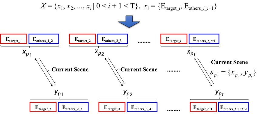
2673

conducts an “Affective Space Mapping”, which particularly extracts emotion features from the given
conversation text collection. In this way, all the conversation texts can be converted into n-dimensional
affective vectors, where each dimension of the affective vector represents the preference to one emotion
category. Based on the affective vector output by the “Affective Space Mapping”, the proposed model
TEP2MP assembles all the affective vectors into multiple data-units, according to the order in which
the conversation text has been published. Here, each data-unit contains the affective vectors of the
corresponding conversation texts, in the form of . In other
words, one data-unit is a combination of one n-dimensional affective vector corresponding to the text
published by the target speaker and m n-dimensional affective vectors of the texts published by all the
other participants. In this way, as shown in Figure 1, the original conversation text collection can be
converted into a time-series particularly on affective vectors and each element in such the time-series
is a basic data-unit formed as .
      Moreover, due to the fact that in the given time-series, there may exist multiple sub-sequences
which present the similar tendency on the shift of emotion category occurring at different intervals [1],
therefore the proposed model TEP2MP takes two adjacent data-units in above time-series as the current
scene, in the form of [t; t+1]. Obviously, the current scene is a sub-sequence consisting of several n-dimensional
affective vectors. Then, according to the current scene, multiple similar scenes will be sought across
the entire conversation history, or the whole time-series, by different time-spans such as day, week and
month. Here, a similar scene is the sub-sequence having similar change on emotion category compared
with that of the current scene. In addition, the similar scenes will be considered as auxiliary features
used to support following text-emotion prediction for target speaker. Finally, the input conversation
text collection, or the time-series consisting of n-dimensional affective vectors, will be aligned up to
the similar scenes, both of which will be fed into a two-layer encoder-decoder prediction model
constructed by Long Short Term Memory (LSTM) [2]. As a result, the emotion of the conversation
text to be published by target speaker in the future can be predicted in a window-rolling manner, even
if the specific content of such the conversation text is still unknown.
      More importantly, in terms of the prediction model constructed as the two-layer encoder-decoder,
emotion fusion mechanism is introduced at the encoder side to merge the n-dimensional affective
vector of the conversation text published by target speaker and those belonging to other participants,
both of which are stored in the same data-unit (i.e., t). The
result of emotion fusion will be forced to be “close” to the n-dimensional affective vector of the
conversation text published by the target speaker in next data-unit. In this way, our proposed prediction
model can capture the emotion interaction among participants at the encoder side as early as possible.
Moreover, at the decoder side, a hybrid attention mechanism is adopted to compute two context vectors
derived from the input conversation text collection and the similar scenes. Such two context vectors
will be merged by a “gate switcher” before fed into decoder, aiming at obtaining critical features on
both the current scene (i.e., derived from the input conversation text) and similar scene to improve the
final performance on text emotion prediction with regard to the target speaker.
      In conclusion, the contribution of this paper is that a text emotion prediction model oriented to
multi-participant text-conversation scenario has been proposed with the support of emotion fusion and
hybrid attention mechanism. The proposed model aims at effectively predicting the emotion of the
conversation text to be published by the target speaker in the future, even if the specific content of the
corresponding conversation text is still unknown. To achieve above goal, first, “Affective Space
Mapping” has been constructed to represent each conversation text as an n-dimensional affective vector

Mathematical Biosciences and Engineering                                      Volume 19, Issue 3, 2671-2699.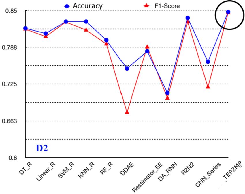
2674

on particular emotion categories. Second, scenes with similar tendency on emotion category shift have
been sought across the entire conversation history to provide auxiliary features for the following
prediction on text emotion. Third, in terms of the emotion interaction among different participants, an
emotion fusion mechanism is adopted at the encoder side to merge the affective vectors corresponding
to the conversation texts posted by different participants, and a hybrid attention mechanism is adopted
at the decoder side to obtain global observation on the current scene and similar scene across the entire
conversation history.

2.   Related works

      In recent years, text sentiment (emotion) analysis has attracted attention from more and more
researchers [3]. Particularly, the general process of text sentiment (emotion) analysis can be described
as: given a collection of texts, the sentiment or emotion category of each text should be recognized
correctly by a classifier, based on the proper text representation. Such the process can also be
considered as text sentiment (or emotion) prediction [4]. In addition, the text representation means the
feature vector of corresponding text which can be obtained by word embedding algorithms (i.e., Skip-
Gram [5]) or other neural components like Auto-Encoder [6]. Moreover, the semantics or syntactics of
given text should also be incorporated into the corresponding representation.
      More importantly, the term “emotion” refers to the intensive and instant feelings such as
happiness, anger, sadness, fear and surprise, etc. [7]. However, the term “sentiment” often means a
feeling or an opinion, especially based on emotions. Typically, in terms of the text sentiment analysis,
the existing models or algorithms often classify the sentiment of corresponding texts as positive,
neutral or negative [8]. Cambria E et al. [9] have constructed a commonsense knowledge base
“SenticNet 6” for sentiment analysis, in which each term has been assigned with a polarity value in
the range of [-1, 1] with the help of logical reasoning by deep learning architectures. It is worthwhile
to be mentioned that, since the sentiment is derived from emotion and it is also feasible to categorize
the specific emotion as “positive” or “negative”, therefore in this paper, we consider the term
“sentiment” and “emotion” as mutually equivalent.
      Specifically, Basiri M E et al. [10] have extracted features from text segments and constructed a
deep bi-directional network with attention mechanism to conduct sentiment prediction. Gong C et al. [11]
have adopted BERT, a pre-trained language model to embed words into vectors, based on which the
semantical dependency between terms can be analyzed. Similarly, Peng H et al. [12] have projected
word representation into a sentiment category space and a mapping function like “word
representation→sentiment category” has been learned. In addition, in order to improve the
effectiveness to capture critical features from the given text, Yang C et al. [13] and Cai H et al. [14]
have adopted Co-Attention Network and Graph Convolutional Network to build the projection from
word embedding to text sentiment category. In terms of the text context, Phan M H et al. [15] have
considered the document being processed as the local context and the given corpora as the global
context. Then, a pre-trained BERT language model is adopted to encode the local and the global
context into vectors, followed by the fusion of above two context vectors via self-attention mechanism,
based on which the sentiment of the given text will be determined.
      Recently, sentiment or emotion analysis in dialog systems has attracted more and more attention.
Typically, Ma et al. [16] have concentrated on the literature of empathetic dialogue system whose goal
is to generate response in a text-conversation scenario with proper sentiment, more adapted to the

Mathematical Biosciences and Engineering                                     Volume 19, Issue 3, 2671-2699.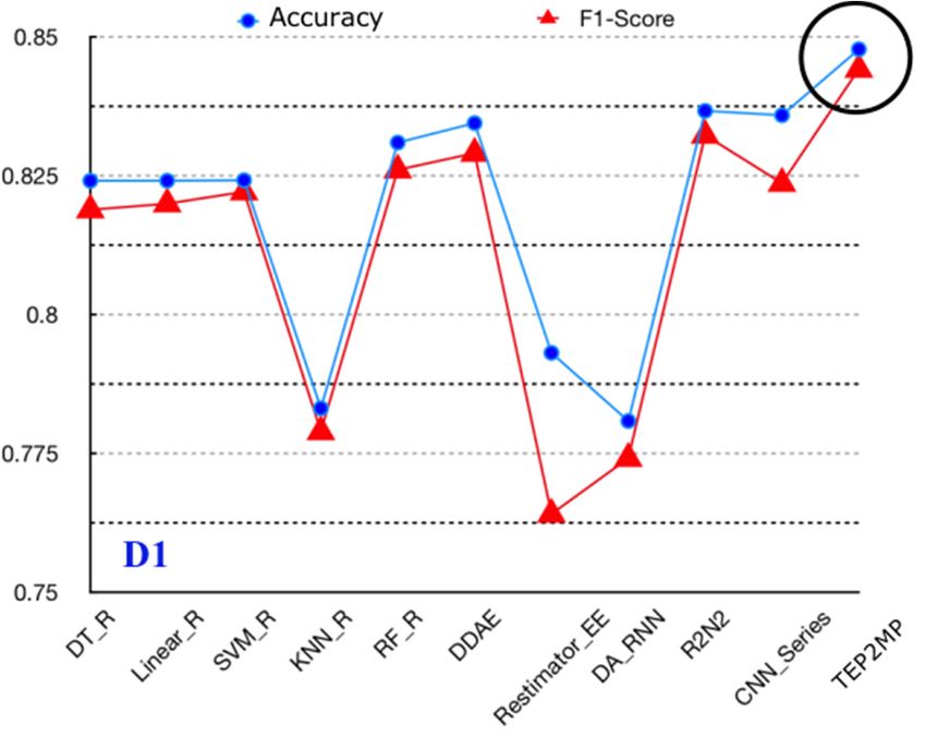
2675

interaction during conversation. In such the survey, emotion-awareness, personality-awareness and
knowledge-accessibility have been considered as three critical factors to enhance the perception and
expression of emotional states. Moreover, Poria S. et al. [17] have also pointed out that the sentiment
reasoning aiming at digging into the detail that causes sentiment is of prime importance with regard to
sentiment perception in dialog systems, whose main purpose is to analyze the motivation behind
sentiment shift via conversation. In order to improve the performance on sentiment analysis in dialog
systems, Li W et al. [18] have proposed a bidirectional emotional recurrent unit (BiERU) whose main
innovation is the generalized recurrent tensor block followed by two-channel classifier designed to
perform context compositionality and sentiment classification simultaneously. In this way, the bi-
directional emotional recurrent unit presents to be fast, compact and parameter-efficient in terms of
conversational sentiment analysis. Similarly, Lian Z et al. [19] have improved the transformer network,
making it more adapted to the conversational emotion recognition, where the conversation texts are
embedded into vectors and the bi-directional recurrent units are utilized to revise above representations
with the help of multi-head attention mechanism. In this way, an emotion classification model on
conversation text can be constructed to determine the specific emotion of each conversation text. In
addition, Zhang Y et al. [20] have utilized the LSTM network, a variant of recurrent-unit-based model,
to capture the interaction during communication so as to realize more precisely conversational
sentiment analysis. Finally, Wang J. [21] have introduced the topic-aware mechanism into the
conversational sentiment analysis, where the sentiment or emotion of each conversation text is
determined based on the text representation, meanwhile the topic of current conversation context
should also be recognized correctly.
      Moreover, in a daily communication scenario, texts are published in sequence. Therefore, the
principle of time-series prediction has offered an inspiration to the task of emotion-prediction in a
multi-participant text-communication scenario. Typically, representative time-series prediction
models are listed as follows. First, a time-series prediction model Attn-CNN-LSTM [22] based on
hybrid neural networks and attention mechanism has been proposed, which conducts “phase
reconstruction” on given time-series. In terms of the prediction, spatial features are extracted first,
followed by the extraction of temporal features via LSTM network. Then, the periodic tendency on
sub-sequence is also mined out, working together with above temporal-spatial features extracted
from the entire time-series so as to enhance the prediction performance. Similarly, an attention-
mechanism based two-phase bi-directional neural network DSTP-RNN [23] conducts time-series
prediction by temporal-spatial features as well. Such the temporal-spatial features are extracted from
the target sequence and the corresponding exogenous sequence across different periods. Besides, the
time-series prediction model DeepAR [24] constructed by auto-regressive recurrent neural network
splits the input sequence into main sequence Z, which contains unknown data point to be predicted.
And, the remaining co-variate sequence X without any unknown data point is taken to assist the
prediction of Z. Such two sequences are aligned up by time step, formed as (z, x), and merged by
Recurrent Neural Network to fit a proper distribution, based on which the unknown data point in main
sequence Z will be predicted. In addition, the Clockwork-RNN network [25] has also been adopted for
time-series prediction [26]. Specifically, temporal features of given time-series are extracted by
Clockwork-RNN. Then, dependencies among data points are learned by traditional feed-forward
neural network with proper distribution fit by Vector Autoregression, based on which a time-series
prediction model has been constructed according to the principle of Stacking ensemble learning [27].
Such the prediction model is required to be fine-tuned by a large amount of high quality data points so

Mathematical Biosciences and Engineering                                     Volume 19, Issue 3, 2671-2699.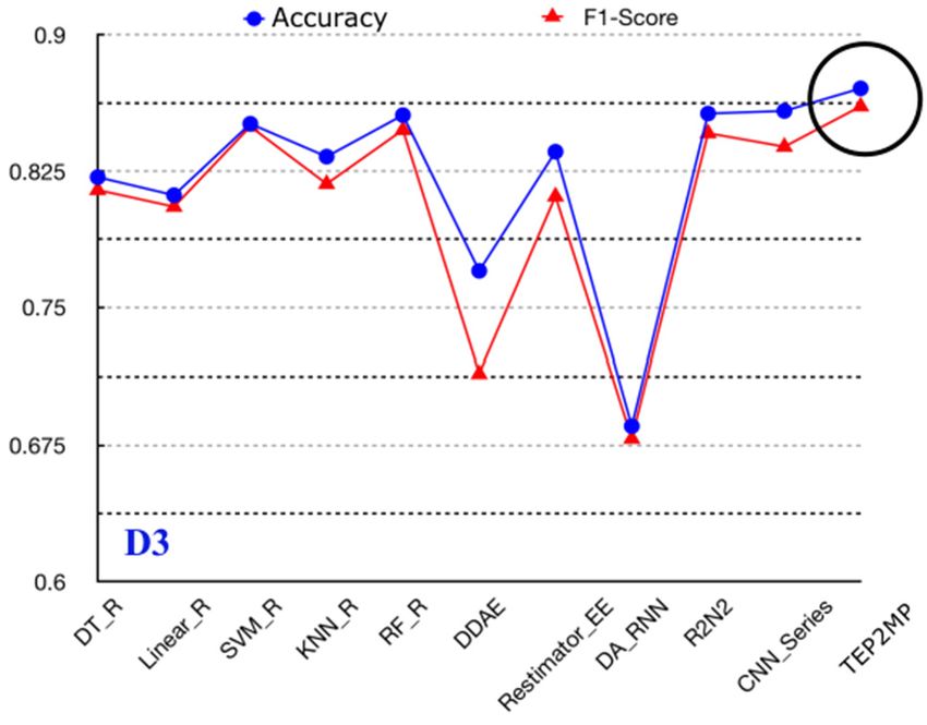
2676

as to obtain stable prediction performance. Finally, a time-series prediction method based on fuzzy
cognitive map, denoted as EMD-HFCM [28] has been proposed which extracts features from the input
sequence by empirical mode decomposition. The extracted features are used to construct high-order
fuzzy cognitive map iteratively used for prediction. Similarly, the prediction model CNN-FCM [29]
adopts residual block to extract features from time-series, and the prediction process is completed by
Fully Connected Neural Network, as a substitute of the fuzzy cognitive map.
      In conclusion, it can be found that existing methods still have two disadvantages with regard to
the text emotion prediction problem in a multi-participant conversation scenario. First, most text
sentiment (emotion) prediction models need to ascertain the text content in advance, then the category
on text sentiment or emotion can be determined by classification. Such requirement has limitation on
real-world application, where the content of the text to be published in the future often presents to be
unknown. Second, the existing time-series prediction model has insufficient consideration on the
similar sub-sequence of the given time-series, resulting in the requirement on a large amount of training
instances to provide more critical features [24]. In other words, sub-sequence with similar tendency
in the given time-series should be analyzed further to provide more auxiliary features available for
final prediction.
      Consequently, in this paper, we convert the text emotion prediction in a multi-participant
conversation scenario into the task of time-series prediction. However, current time-series model
conducts prediction mainly by analyzing the tendency on target variable, not involved with the
processing on sentiment or emotion interaction among different participants. In other words, existing
time-series prediction models can not be applied directly. Therefore, effort should be devoted to
construct more advanced time-series-based text emotion prediction model, making it more adapted to
the multi-participant text conversation scenario.

3.    The proposed method

3.1. Text affective space mapping

      In this paper, we focus on the text-emotion prediction task in a multi-participant conversation
scenario, whose ultimate goal is to correctly categorize the emotion or sentiment of the conversation-
text to be posted in the future. Consequently, the conversation text should be first represented or
embedded into vectors so as to be analyzed further [3,4]. However, different from the existing
embedding algorithms [5,6], whose principle is to “shorten” the vector distance for terms semantically
related or similar, features on emotion or sentiment should also be incorporated into text representation
in order to enhance the emotion prediction performance. Therefore, we first turn to “Affective Space
Mapping”, aiming at obtaining text representation containing details on corresponding emotion or
sentiment categories.
      It is obvious that, by the time at which the text has been published, the original conversation text
collection can be converted into a sequence, like D = {d1, d2, ..., di|0 < i + 1 < T}. Here di represents a
single text published by one participant in the conversation. And, the process of Affective Space
Mapping on text has been illustrated in Figure 2.

Mathematical Biosciences and Engineering                                       Volume 19, Issue 3, 2671-2699.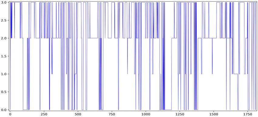
2677

   ①Conduct emotion category annotation                  ④Train Bi-LSTM based emotion classifier;

   and publisher annotation on the original                Obtain n-dimensional affective vector for

        conversation text sequence D.                              every conversation text;

        ②Compute the global emotion                     ⑤Revise the n-dimensional affective vector of

    interaction pattern EIP for the original            every conversation text, output by Bi-LSTM,
        conversation text sequence D.                                   via global EIP.

   ③Tokenize texts in original conversation                ⑥Convert the original conversation text

      text sequence D into words; Obtain                 sequence D into a sentimental time-series
        corresponding word embeddings.                   consisting of n-dimensional affective vectors

                           Figure 2. The process of Affective Space Mapping.

       First, the sentiment or emotion of the original conversation text sequence D = {d1, d2, ..., di|0 < i
+ 1 < T} will be annotated like [Target_Flag, Emotion_Index]. Here, Target_Flag (0/1) means if the
current text is published by the target speaker (i.e., 1 for target speaker) and the Emotion_Index means
the specific sentiment or emotion category annotated for each conversation text. Based on the text
sentiment or emotion annotation, the original conversation text sequence D = {d1, d2, ..., di|0 < i + 1 <
T} can be converted into an Emotion Category Sequence, in which each element is the Emotion_Index
or the specific emotion category of the corresponding conversation text.
       Second, as shown in Algorithm 1, the global Emotion Interaction Pattern (EIP) [30] of the original
conversation text sequence D will be computed based on above Emotion Category Sequence. Here,
the global EIP is used to depict the distribution on n emotion categories in terms of the entire original
conversation text sequence D = {d1, d2, ..., di|0 < i + 1 < T}.
       In Algorithm 1, at step 1, a global emotion interaction dictionary dict is initialized by n emotion
categories (e1, e2, ..., en). In terms of such the dict, each emotion category e has its own n-dimensional
list, initialized as [0, 0, ...0]∈Rn, which represents the co-occurrence frequency with other emotion
categories when encountering an emotion category e in the original conversation text sequence D. In
this way, the interaction among different emotion categories can be incorporated in one EIP dictionary.
At Step 2, a time-window with size 2, stride 1 has been created. Such the time-window is used to scan
the whole Emotion Category Sequence like (Emotion_Indexi, Emotion_Indexj), based on which the ith
and jth dimension of the n-dimensional list of emotion category ei is updated (i.e., add 1 frequency
count) to revise the global EIP dictionary dict. Finally, at Step 3, when the above time-window has
moved to end of Emotion Category Sequence, “softmax” operation is conducted towards all the n-
dimension list in the global EIP dictionary to obtain the final normalized EIP matrix, which can be
considered as the emotion distribution on n emotion categories in terms of the given conversation text
sequence D. Specifically, when selected four emotions such as “happy”, “sad”, “angry” and “other”,

Mathematical Biosciences and Engineering                                       Volume 19, Issue 3, 2671-2699.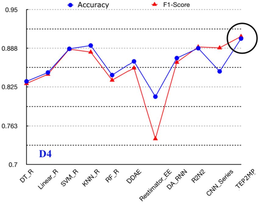
2678

the global EIP output by Algorithm 1 is shown in Figure 3 and the index of the maximum value in each
line of EIP represents the corresponding emotion category.

                  Algorithm 1. The process to compute the global Emotion Interaction Pattern.
Input: The Emotion Category Sequence corresponding to the original conversation text sequence D
Output: The global EIP of the original conversation text sequence D
1. Select n emotion categories (e1, e2, ..., en) and initialize the global EIP dictionary as follows:
    dict = {e1:[0, 0, ..., 0], e2:[0, 0, ..., 0], ..., en:[0, 0, ..., 0]};
2. Create a time-window with size=2, stride=1 to scan the entire Emotion Category Sequence. Revise the global EIP
dictionary according to the pair of emotion category (i.e., e1, e2) in the current time-window, as:
     ① (Emotion_Index1, Emotion_Index2) → dict = {e1: [1, 1, ..., 0], e2: [0, 0, ..., 0], ..., en: [0, 0, ..., 0]};
     ② (Emotion_Index2, Emotion_Indexn) → dict = {e1: [1, 1, ..., 0], e2: [0, 1, ..., 1], ..., en: [0, 0, ..., 0]};
     ③ (Emotion_Indexn, Emotion_Index2) → dict = {e1: [1, 1, ..., 0], e2: [0, 1, ..., 1], ..., en: [0, 1, ..., 1]};
     ④ (Emotion_Index2, Emotion_Index1) → dict = {e1: [1, 1, ..., 0], e2: [1, 2, ..., 1], ..., en: [0, 1, ..., 1]};
     .............................
3. Repeat Step 2, scanning to the end of Emotion Category Sequence by moving above time window with stride = 1,
revising the global EIP dictionary according to the pair of emotion category (i.e., e1, e2) in the current time-window
iteratively;
4. Normalize the global EIP dictionary by “softmax”, which is output as the final global EIP of the original conversation
text sequence D;

                                              Figure 3. The example of global EIP.

      Third, in terms of the Affective Space Mapping as shown in Figure 2, the original conversation
text in sequence D will be tokenized into words, which are then embedded into vectors by Skip-gram [5]
iteratively. Fourth, based on above word vectors, the original conversation text sequence D will be fed
into Bi-LSTM [18] to be represented as a sequence of word vectors. Here, the adopted Bi-LSTM works
as an n emotion category classifier. Then, the trained Bi-LSTM will be reused to compute the emotion
distribution on n emotion categories (with softmax normalization) for each conversation text in D. In

Mathematical Biosciences and Engineering                                                        Volume 19, Issue 3, 2671-2699.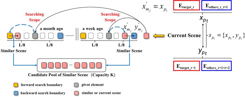
2679

this way, the normalized n-dimension emotion distribution, or affective vector, for each conversation
text can be obtained. Fifth, for every conversation text in sequence D, the index of the maximum value
of the n-dimensional affective vector will be checked, ensuring the consistency to the Emotion_Indexi
annotated at the beginning. If a conflict occurred, then according to the Emotion_Indexi annotated
before, the corresponding n-dimensional list in EIP as shown in Figure 3 will be extracted, working as
a substitution of the n-dimensional affective vector of the current conversation text. Finally, the original
text conversation sequence D can be represented as a sequence of n-dimensional affective vectors,
denoted as D’ = {E1, E2, ..., Ei, Ei = (e1, e2, ..., en)∈Rn|0 < i + 1 < T, en∈R}, where each Ei = (e1, e2, ...,
en)∈Rn is an n-dimensional affective vector.
      More importantly, at the final step of Affective Space Mapping as shown in Figure 2, according
to the Target_Flag (0/1) annotated at the beginning, all the n-dimensional affective vectors
corresponding to the conversation texts published by the target speaker (Target_Flag = 1) will be
extracted from D’ = {E1, E2, ..., Ei, Ei = (e1, e2, ..., en)∈Rn |0 < i + 1 < T, en∈R}, denoted as D’target =
{Etarget_1, Etarget_2,...,Etarget_i|0 < i + 1 < T, Etarget_i∈Rn}. Here, Etarget_i refers to an n-dimensional affective
vector of the conversation text published by the target speaker at time step i. Moreover, in terms of the
adjacent time step i and i + 1, all the texts published by other participants between time step i and i + 1
will be collected and the corresponding n-dimensional affective vector collection between time step i
and i + 1 is denoted as Eothers_i_i+1. As a result, the n-dimensional affective vector corresponding to the
conversation text published by target speaker at time step i (i.e., Etarget_i), along with a set of n-
dimensional affective vectors derived from the conversation texts published by all the other participants
between time step i and i + 1 will be assembled into a basic data-unit altogether, denoted as xi = {Etarget_i,
Eothers_i_i+1}.
      After Affective Space Mapping illustrated in Figure 2, the original conversation text sequence D
will be converted into a time-series X = {x1, x2, ..., xi|0 < i + 1 < T}, consisting of multiple n-dimensional
affective vectors. Each element in time-series X is xi = {Etarget_i, Eothers_i_i+1}, which is a basic data-unit
containing n-dimensional affective vectors corresponding to the target and other participants between
the adjacent time step i and i + 1.

3.2. Similar scene search and attention sequence extraction

     As mentioned above, after Affective Space Mapping, the original conversation text sequence D
can be represented as a time-series X = {x1, x2, ..., xi|0 < i + 1 < T}, consisting of multiple n-dimensional
affective vectors. Particularly, every element in the input series X is a basic data-unit, or a sub-sequence,
like xi = {Etarget_i, Eothers_i_i+1}, which contains one n-dimensional affective vector of the conversation
text published by the target speaker at time step i and a set of n-dimensional affective vectors of texts
published by all the other participants between time step i and i + 1.
     Generally, most time series may have pseudo-periodicity, which means several sub-sequences
may present similar tendency on the change of values, occurring at regular or irregular intervals [31].
Such the similar sub-sequence brought about by the pseudo-periodicity can provide extra features for
the prediction of the given time-series [32]. Consequently, inspired by such principle, when it comes
to the time-series X = {x1, x2, ..., xi|0 < i + 1 < T} derived from the multi-participant text-conversation
scenario, although the shift among different sentiment or emotion categories may not present to be
periodical, yet there may exist several sub-sequences containing similar tendency on the emotion
category shift to that of the given sub-sequence xi = {Etarget_i, Eothers_i_i+1}. For instance, the emotion of
the target speaker could shift from “sad” to “angry” at different time steps across the entire

Mathematical Biosciences and Engineering                                              Volume 19, Issue 3, 2671-2699.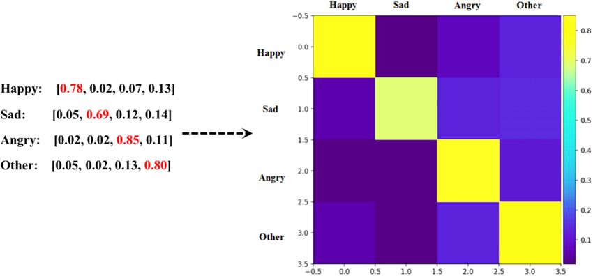
2680
conversation history. Therefore, sub-sequences with similar tendency on emotion category shift should
be collected for the given sub-sequence xi = {Etarget_i, Eothers_i_i+1} for further processing, so that more
auxiliary features can be collected for analyzing the sub-sequence xi = {Etarget_i, Eothers_i_i+1}.
Based on above inspiration, as shown in Figure 4, when given the input time-series X = {x1, x2, ...,
xi|0 < i + 1 < T}, where xi = {Etarget_i, Eothers_i_i+1}, an input sequence X P {x p1 , x p2 ,..., x pt , pt T }
spanning pt time steps will be selected from X. Here, each element in Xp can be represented as
x pt {Etarget_t , Eothers _ t _ t 1} . Then, a target sequence YP { y p1 , y p2 ,..., y pt , pt T } , or the ground truth
to be predicted later, will also be selected from X. It should be noted that the start point of the target
sequence Yp is the time step of x p2 in Xp and the target sequence Yp spans pt time steps as well. In other
words, for y pt {Etarget_t 1 , Eothers _ t 1_ t 2 } , y p1 x p2 , y p2 x p3 , ..., y pt x pt 1 , the target sequence Yp
is actually obtained by shifting the input sequence Xp one time step forward, in the direction to t+1.
Finally, as shown in Figure 4, the current scene (or a sub-sequence) can be constructed as the
combination of one element in Xp and another element in Yp, denoted as s pt {x pt , y pt } .
Figure 4. The construction of current scene from the given sentimental time-series X.
In this way, when given the input sequence X P {x p1 , x p2 ,..., x pt , pt T } and a target sequence
YP { y p1 , y p2 ,..., y pt , pt T } , t current scenes (or sub-sequences) in all will be extracted from the entire
time-series X = {x1, x2, ..., xi|0 < i + 1 < T}, where xi = {Etarget_i, Eothers_i_i+1}. Here,
x pt {Etarget_t , Eothers _ t _ t 1} , y pt {Etarget_t 1 , Eothers _ t 1_ t 2 } .
Moreover, in terms of the input time-series X = {x1, x2, ..., xi | 0 < i + 1 < T} where xi = {Etarget_i,
Eothers_i_i+1}, as shown in Figure 5, a period-offset searching method is adopted to extract multiple
similar scenes (or several sub-sequences) from the input time-series X by different periods (i.e., day,
week or month), according to the given current scene (sub-sequence) s pt {x pt , y pt } . Here, the
extracted similar scenes must have the similar change on emotion categories compared to that of the
current scene s pt {x pt , y pt } . More specifically, when given a current scene s pt {x pt , y pt } ,
x pt {Et arg et _ t , Eothers _ t _ t 1} and y pt {Etarget_t 1 , Eothers _ t 1_ t 2 } , K similar scenes (sub-sequences),
denoted as sm { xm' j , ym' j } , j∈[1,K], will be extracted from the input time-series X = {x1, x2, ..., xi
Mathematical Biosciences and Engineering Volume 19, Issue 3, 2671-2699.2681
|0 < i + 1 < T}, xi = {Etarget_i, Eothers_i_i+1}, satisfying the requirement that xm' j {Etarget_j , Eothers_j_j 1} ,
ym' j {Etarget_j 1 , Eothers_j 1_j 2 } , and xm' j x pt . .
Figure 5. The searching of similar scenes according to the given current scene.
More explicitly, as illustrated in Figure 5, when given a current scene s pt {x pt , y pt } , the adopted
period-offset searching method will find a pivot element at first, which is a similar sub-sequence
nearest to the current scene s pt {x pt , y pt } across the input time-series X. For instance, in Figure 5, a
pivot element is first found by week. Then, starting from the pivot element, a searching scope with
size L/8 will be expanded from left and right respectively, in which an element xm' j most similar to
x pt in s pt {x pt , y pt } will be determined and the next element ym' j is taken to construct a similar
scene (sub-sequence) like sm { xm' j , ym' j } . Such the similar scene will be stored in a pool of candidate
similar scene with capacity K. Repeating above searching process, traversing the entire time-series X
by different time periods (i.e., day, week and month) until the amount of the candidate similar scenes
has achieved the threshold K, in this way, K similar scenes (sub-sequences) corresponding to the
current scene (sub-sequence) s pt {x pt , y pt } will be obtained by different periods, denoted as
sm { xm' j , ym' j } , j∈[1, K]. In conclusion, for each current scene (sub-sequence) s pt {x pt , y pt } , where
x pt {Et arg et _ t , Eothers _ t _ t 1} and y pt {Etarget_t 1 , Eothers _ t 1_ t 2 } , a set of K similar scenes (sub-sequences)
sm { xm' j , ym' j } , j∈[1, K] will be extracted from the input time-series X by the period-offset searching
method as shown in Figure 5. Here, xm' j {Etarget_j , Eothers_j_j 1} , ym' j {Etarget_j 1 , Eothers_j 1_j 2 } , and
xm' j x pt .
In addition, when given a current scene s pt {x pt , y pt } , along with a set of K similar scenes,
where sm {xm' j , ym' j } , j∈[1, K] , an attention vector of the current scene s pt {x pt , y pt } towards K
similar scenes will be computed via the element y pt in the current scene s pt {x pt , y pt } and all the
elements ym' j , j∈[1, K], in the corresponding K similar scenes, denoted as s pt {x pt , y pt } at in Eq (1).
Therefore, the attention vector at represents the observation from the element y pt in current scene
s pt {x pt , y pt } towards all the corresponding elements ym' j , j∈[1, K] in similar scenes.
Mathematical Biosciences and Engineering Volume 19, Issue 3, 2671-2699.2682
etj va tanh(Wpt y pt Wm j ym j bpt )
T '
exp(etj )
tj K (1)
j '1 etj '
K
a y ' s {x , y }
t tj mj pt pt pt
j 1
In this way, as shown in Figure 4, when given an input sequence X p {x p1 , x p2 ,..., x pt , pt T }
selected from X and the corresponding target sequence Yp { y p1 , y p2 ,..., y pt , pt T } which is the
ground truth of prediction, t current scenes (i.e., s pt {x pt , y pt } ) will be created immediately. For each
current scene, the period-offset searching method as shown in Figure 5 will be adopted to extract K
similar scenes (i.e., sm {xm' j , ym' j } , j ∈ [1, K] ) from the input time-series X, followed by the
observation from y pt to ym' j , j∈[1, K], so as to obtain the attention vector at of the current scene
s pt {x pt , y pt } derived from K similar scenes as defined in Eq (1). Furthermore, for the t current
scenes, an attention-feature sequence can be obtained, denoted as A= {a1, a2, ..., at, t∈T}. Such the
attention-feature sequence can be considered as the auxiliary feature of the input sequence
X p {x p1 , x p2 ,..., x pt , pt T } to support following emotion prediction. Finally, the attention-feature
sequence A= {a1, a2, ..., at, t∈T}, the input sequence X p {x p1 , x p2 ,..., x pt , pt T } along with the
target sequence Yp { y p1 , y p2 ,..., y pt , pt T } will be aligned up by time step.
3.3. Two-layer encoder-decoder with emotion fusion and hybrid attention
Generally, the proposed model TEP2MP conducts text emotion prediction in a multi-participant
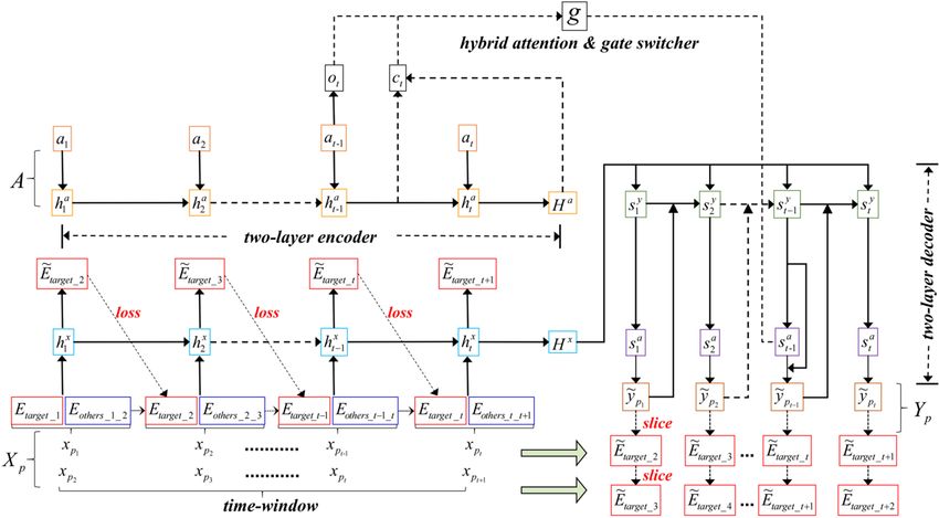
communication scenario by the two-layer encoder-decoder prediction model as shown in Figure 6.
First, the prediction model in Figure 6 consists of the encoding and decoding phase. Specifically, the
prediction model encodes the input sequence X p {x p1 , x p2 ,..., x pt , pt T } and the attention-feature
sequence A= {a1, a2, ..., at, t∈T} via two-layer bi-directional LSTM. Here, at the encoding stage, the
input sequence Xp and the attention-feature sequence A have been aligned up by time step. For decoder,
on the one hand, the two-layer decoder decodes the input sequence Xp step by step to obtain the hidden
state sty at time step t. On the other hand, the hybrid attention mechanism has also been introduced to
compute the context vector ot corresponding to the attention-feature sequence A= {a1, a2, ..., at, t∈T}
and the context vector ct corresponding to the input sequence Xp. Such two context vectors will be
merged by the gate switcher g to obtain another hidden state derived from the hybrid attention
mechanism at different time steps, denoted as g(ot, ct)→ sta . Finally, the prediction result
~ ~ ~
y {E
pt ,E
t arg et _ t 1 } will be output step by step according to the hidden state s y and s a .
others _ t 1 _ t 2 t t
~
Obviously, the predicted n-dimensional affective vector Etarget _ t 1 in the prediction result
~ ~ ~
y pt {Et arg et _ t 1 , Eothers _ t 1 _ t 2 } is corresponding to the conversation text published by the target
speaker at t+1 time step, which should be close to the element Etarget_t+1 in the sub-sequence
Mathematical Biosciences and Engineering Volume 19, Issue 3, 2671-2699.2683
y pt {Et arg et _ t 1 , Eothers _ t 1_ t 2 } . Here, y pt is an element in the target sequence Yp, or the ground truth
~
of the predicted Etarget _ t 1 .
Figure 6. The structure of the two-layer encoder-decoder prediction model.
Moreover, in Figure 6, a time-window spanning t time steps will be set before prediction, based
on which the two-layer encoder-decoder will select the corresponding input sequence
X p {x p1 , x p2 ,..., x pt , pt T } and target sequence Yp { y p1 , y p2 ,..., y pt , pt T } (the ground truth of
prediction) from the given time-series X = {x1, x2, ..., xi|0 < i + 1 < T}, where xi = {Etarget_i, Eothers_i_i+1}.
Here, y pt = x pt 1 , y pt {Et arg et _ t 1 , Eothers _ t 1_ t 2 } . In other words, the target sequence Yp is obtained by
shifting the input sequence Xp one time step forward, along the direction to t+1. And, the n-dimensional
affective vector Etarget_t+1 in y pt {Etarget _ t 1 , Eothers _ t 1_ t 2 } is corresponding to the emotion of the text to
be published by the target speaker at time step t + 1. Obviously, the target sequence Yp can be
~
considered as the ground truth of the predicted sequence Y p { ~
y p1 , ~
y p2 ,..., ~
y pt , pt T } output by the
tow-layer decoder. Furthermore, as shown at the bottom of Figure 6, when the time-window moves
forward by the fixed stride, the input sequence Xp will move towards the end of the given time-series
X. As a result, the emotion of the text to be published by the target speaker from time step t + 2 → t +
N will be predicted in sequence.
~
htx LSTM ( FC ( x pt {Et arg et _ t , Eothers _ t _ t 1}), htx1 ) Et arg et _ t 1 (2)
1 ~
(E
t
l1 t arg et _ t 1 Et arg et _ t 1 ) 2 (3)
t 1
In addition, as shown in Figure 6, after selecting the input sequence Xp, the emotion fusion
mechanism will be incorporated into the first-layer encoder. Here, the first-layer encoder is the LSTM
Mathematical Biosciences and Engineering Volume 19, Issue 3, 2671-2699.2684
network. And, as defined in Eq (2), the emotion fusion mechanism will merge the n-dimensional
affective vector Etarget_t and Eothers_t_t+1 in x pt {Etarget _ t , Eothers _ t _ t 1} by fully connected layer, after which
the emotion fusion result will be further processed by LSTM (the second-layer encoder), denoted as
~ ~
Etarget _ t 1 . Here, the emotion fusion result Etarget _ t 1 will be forced to approach the n-dimensional
affective vector Etarget_t+1 (the affective vector of the conversation text to be published by the target
speaker at next time step t + 1). Finally, the loss l1 defined in Eq (3) will be adopted to measure the
difference between emotion fusion result and the ground truth of the affective vector input at the next
time step. In this way, by incorporating the emotion fusion mechanism into the first-layer encoder and
forcing the emotion fusion result to approach the ground truth of the affective vector corresponding to
the conversation text published by the target speaker at next time step, the prediction model in Figure 6
will be guided to learn emotion interaction among the target speaker and all the other participants so
as to capture the emotion stimulation to the target speaker triggered by the other participants.
Afterwards, when given the input sequence X p {x p1 , x p2 ,..., x pt , pt T } , a hidden state sequence
will be output by the first-layer encoder (i.e., LSTM), denoted as H x {h1x , h2x ,..., htx } . Similarly, the
second-layer encoder (i.e., another LSTM) will encode the attention-feature sequence A = {a1, a2, ...,
at, t∈T}, derived from the similar scene searching process illustrated in Figure 5 so as to obtain the
corresponding hidden state sequence H a {h1a , h2a ,..., hta } .
sty LSTM ( ~
y pt1 , sty1 , H x ) (4)
At the decoding stage, as shown in Figure 6, first, when given the hidden state sequence
H {h1x , h2x ,..., htx } derived from the input sequence Xp, the top-layer decoder (i.e., LSTM) will decode
x
the hidden state step by step, denoted as s y at time step t as defined in Eq (4). Here, in Eq (4), ~
t y is pt 1
the prediction result output by the decoder at time step t-1.
ot (Wa at bt )
ct t tanh( H )
x
(5)
y
t Attn(WH H Ws st b )
x
Moreover, as shown in Figure 6, a hybrid attention mechanism has been adopted. Specifically, as
defined in Eq (5), the context vector ot at time step t will be computed based on the attention vector at,
when given the hidden state sequence H a {h1a , h2a ,..., hta } derived from the attention-feature sequence
A={a1, a2, ..., at, t∈T}. Similarly, the context vector ct at time step t will be computed by aggregating
the hidden state sequence H x {h1x , h2x ,..., htx } weighted by the attention-weight γ. Such the attention-
weight γ is involved with the hidden state sty . In this way, as shown in Figure 6, when decoding at
time step t, the hidden state sta will be computed by absorbing the context vectors ot and ct via the
~ ~
gate switcher g, as defined in Eq (6). And, the emotion prediction result ~y pt {Etarget _ t 1 , Eothers _ t 1 _ t 2 }
output at time step t will be computed based on the two hidden states sty and sta .
Mathematical Biosciences and Engineering Volume 19, Issue 3, 2671-2699.2685
g (Wh hta Wsg sty bg )
a
s t (1 g ) ot g ct (6)
~
y pt (Ws st Ws st by )
y y a a
~
Finally, as shown in Figure 6, an operation slice ( ~y pt ) Etarget _ t 1 has been defined, where
~ ~ ~
y pt {Etarget _ t 1 , Eothers _ t 1 _ t 2 } . Moreover, similar to Eq (3), the loss l2 is computed to measure the
~
difference between the emotion prediction result Etarget _ t 1 and the corresponding ground truth
Etarget_t+1. Consequently, the two-layer encoder-decoder model will be trained by LOSS=λ1l1+λ2l2 to
enhance the emotion prediction performance. Here, l1 represents the “loss” on emotion fusion (defined
in Eq (3)), aiming at guiding the two-layer encoder to capture the emotion interaction among multiple
participants. And, l2 represents the “loss” on emotion prediction of the two-layer decoder, aiming at
forcing the emotion prediction result decoded at time step t to be “close” to the true n-dimensional
affective vector corresponding to t + 1 time step.
4. Experimental results
In this section, the experimental results on the proposed text emotion prediction model TEP2MP
will be analyzed. The impact of the time-window size, time-window stride, the searching scope of
similar scenes, the capacity of the pool to store candidate similar scenes, the hybrid attention and
emotion fusion mechanism incorporated in the two-layer encoder-decoder prediction model will also
be discussed. Moreover, the existing time-series models which can be adapted to the text emotion
prediction problem have also been compared. All the involved experiments are conducted via 5-fold
cross validation and the average of three times running has been presented. In addition, when it comes
to the proposed text emotion prediction TEP2MP, a four-layer bidirectional LSTM has been adopted
to construct the two-layer encoder-decoder prediction model illustrated in Figure 6, and RELU [33] is
used for neural activation trained by the RMSPropOptimizer [34] with learning rate set as 7 × 10⁻³.
The proposed model TEP2MP and the compared methods are all implemented by Python 3.7 and
Tensorflow 1.15, on GPU, NVIDIA GeForce GTX 1080Ti, 11GB.
4.1. Dataset and emotion annotation
In order to reproduce a multi-participant text conversation scenario, four collections of movie
lines are adopted. In terms of the participants of conversation, we take the main movie character as the
target speaker and the remaining as other participants. The specific information of the four text
collections are shown in Table 1. Here, for the following part of this section, “Gump.” is used to
represent dataset 1, “Shawshank.” for dataset 2, “Scent.” for dataset 3, “Bovary.” for dataset 4 due to
the limited space.
In terms of the emotion category, we annotate the emotion of texts contained in above four
datasets as [Target_Flag (0/1), Emotion_Index (1~6)]. Here, the Emotion_Index (1~6) represents
“Happy”, “Sad”, “Angry”, “Anxious”, “Surprise” and “Other” respectively. The emotion distribution
on the involved datasets is shown in Table 2. The annotation processing is completed by five
researchers with experience in Natural Language Processing and Time-Series Prediction. And, the
Mathematical Biosciences and Engineering Volume 19, Issue 3, 2671-2699.2686
majority voting mechanism has been adopted to determine the final emotion of each text with the
agreement from at least three annotators. Based on above annotation, the Affective Space Mapping
illustrated in Figure 2 has been conducted, in which word embeddings with 256 dimensions have been
used. In addition, the accuracy of the emotion classifier (i.e., Bi-LSTM) has been maintained by 80%
and more. The affective vectors classified incorrectly are revised by the global emotion EIP. The
specific statistics on emotion annotation has been demonstrated in Figure 7. More specifically, Figure
7(a) represents the annotation distribution on six emotion categories (i.e., Happy, Sad, Angry, Anxious,
Surprise and Other) in terms of the conversation texts posted by all the participants, while Figure 7(b)
represents the emotion distribution of the conversation texts particularly posted by the target speaker.
Correspondingly, Figure 7(c),(d) represent the annotation shift on above six emotion categories with
regard to Figure 7 (a),(b) respectively.
Table 1. Experimental datasets for testing TEP2MP.
No. Movie Name Prediction Target Movie Duration #Total Text #Text of Target Speaker
1 Forrest Gump Forrest Gump 142 min 2054 905
2 Shawshank Redemption Ellis Boyd Redding 142 min 1729 590
3 Scent a of Woman Lieutenant Frank 157 min 2226 1165
4 I Am Not Madame Bovary XueLian Li 138 min 2323 505
Table 2. Emotion category distribution after annotation of different datasets.
No. Dataset Statistical Scope Happy (%) Sad (%) Angry (%) Anxious (%) Surprise (%) Other (%)
1 Gump. 40.70 17.96 10.81 18.16 1.36 11.00
2 Shawshank. ALL Conversation42.34 12.78 21.75 12.67 0.29 10.18
3 Scent. Participants 31.18 12.8 28.26 18.28 1.08 8.40
4 Bovary. 13.78 6.03 43.65 ------- ------- 36.55
No. Dataset Statistical Scope Happy (%) Sad (%) Angry (%) Anxious (%) Surprise (%) Other (%)
1 Gump. 47.29 22.54 0.88 17.35 0.55 11.38
2 Shawshank. 58.31 19.83 5.93 7.97 0.51 7.46
Only Target Speaker
3 Scent. 35.45 18.03 29.18 4.03 0.34 12.96
4 Bovary. 9.11 7.33 74.06 ------- ------- 9.50
In terms of the emotion category, we annotate the emotion of texts contained in above four
datasets as [Target_Flag (0/1), Emotion_Index (1~6)]. Here, the Emotion_Index (1~6) represents
“Happy”, “Sad”, “Angry”, “Anxious”, “Surprise” and “Other” respectively. The emotion distribution
on the involved datasets is shown in Table 2. The annotation processing is completed by five
researchers with experience in Natural Language Processing and Time-Series Prediction. And, the
majority voting mechanism has been adopted to determine the final emotion of each text with the
agreement from at least three annotators. Based on above annotation, the Affective Space Mapping
illustrated in Figure 2 has been conducted, in which word embeddings with 256 dimensions have been
used. In addition, the accuracy of the emotion classifier (i.e., Bi-LSTM) has been maintained by 80%
and more. The affective vectors classified incorrectly are revised by the global emotion EIP. The specific
statistics on emotion annotation has been demonstrated in Figure 7. More specifically, Figure 7 (a)
represents the annotation distribution on six emotion categories (i.e., Happy, Sad, Angry, Anxious,
Surprise and Other) in terms of the conversation texts posted by all the participants, while Figure 7 (b)
represents the emotion distribution of the conversation texts particularly posted by the target speaker.
Mathematical Biosciences and Engineering Volume 19, Issue 3, 2671-2699.2687
Correspondingly, Figure 7(c),(d) represent the annotation shift on above six emotion categories with
regard to Figure 7(a),(b) respectively.
(a) (b)
(c)
(d)
Figure 7. The visualization of emotion distribution after annotation: (a) The emotion
distribution of the initial text set D. (b) The emotion distribution of target participant. (c) The
emotion tendency on the initial text set D. (d) The emotion tendency on target participant.
Mathematical Biosciences and Engineering Volume 19, Issue 3, 2671-2699.2688
4.2. The impact of the similar scene searching to the emotion prediction
When given the input sequence Xp and the target sequence Yp (the ground truth of prediction), t
current scenes will be created. After the similar scene searching process illustrated in Figure 4 and
Figure 5, the period-offset searching method will seek K similar scenes for each current scene. Such
the K similar scenes will be aggregated into an attention vector at, then an attention-feature sequence
A= {a1, a2, ..., at, t∈T} will be computed corresponding to the t current scenes. Here, the attention-
feature sequence A= {a1, a2, ..., at, t∈T} will be aligned up to the input sequence Xp by time steps,
which is further taken as the auxiliary features input into the encoder at the second-layer shown in
Figure 6. Moreover, for each current scene in Figure 5, the period-offset searching method will expand
a searching scope L/8 from left and right respectively after a pivot element has been found out by
different time spans. When it comes to the experiments involved in this section, 5 minute is adopted
to search K similar scenes according to the timestamp of each text in datasets.
Table 3. The impact of similar scene search mechanism on the text emotion prediction
accuracy of TEP2MP model (K = 5, λ1 = λ2= 0.5).
Optimal Time
Dataset The Searching Scope L and Optimal Value Accuracy F1-Score
Window
L = win × 0 = 0 (No Similar Scene Search) 0.602039 0.602931
L = win × 4 = 8 0.652314 0.662319
1-Gump win = 2 L = win × 16 = 32 0.782182 0.783418
L = win × 64 = 128 0.832741 0.826231
L = win × 256 = 512 0.801248 0.803583
The improvement on prediction precision(%) +27.70% +27.03%
L = win × 0 = 0 (No Similar Scene Search) 0.623042 0.624617
L = win × 4 = 12 0.702144 0.704294
2-Shawshank win = 3 L = win × 16 = 48 0.762024 0.770214
L = win × 64 = 192 0.849317 0.846003
L = win × 256 = 768 0.810423 0.814956
The improvement on prediction precision(%) +26.64% +26.17%
L = win × 0 = 0 (No Similar Scene Search) 0.759301 0.751280
L = win × 4 = 12 0.810493 0.819203
3-Scent win = 3 L = win × 16 = 48 0.839301 0.830382
L = win × 64 = 192 0.845665 0.841092
L = win × 256 = 768 0.823540 0.824765
The improvement on prediction precision(%) +11.37% +11.95%
L = win × 0 = 0 (No Similar Scene Search) 0.798394 0.793829
L = win × 4 = 16 0.813894 0.812405
4-Bovary win = 4 L = win × 16 = 64 0.853919 0.852834
L = win × 64 = 256 0.866187 0.855451
L = win × 256 = 1024 0.859301 0.853526
The improvement on prediction precision(%) +7.83% +7.20%
In order to measure the impact of L/8 searching scope on the emotion prediction performance, the
Mathematical Biosciences and Engineering Volume 19, Issue 3, 2671-2699.2689
capacity of the pool to store similar scenes is set as K = 5 and the optimal value of L is selected by grid
search, stopping at the first option when the prediction performance decreases. More importantly, for
the LOSS = λ1l1 + λ2l2 used for training the TEP2MP, λ1 and λ2 are set as 0.5. Particularly, when L = 0,
no similar scene will be searched for each current scene. The specific emotion prediction performance
is shown in Table 3.
As shown in Table 3, first, the optimal size of time-window on each dataset is selected by grid
search. Second, based on the optimal time window size, taking the main character on each dataset as
the target speaker and the remaining characters as the other participants, the optimal searching scopes
are listed as 1-Gump, win = 2, L = 128; 2-Shawshank, win = 3, L = 192; 3-Scent, win = 3, L = 192; 4-
Bovary, win = 4, L = 256. Third, compared with the case when L = 0 (i.e., no similar scene has been
searched), it can be observed that when adopting the similar scene searching mechanism, the precision
on text-emotion prediction has been improved by approximately 10%~30%. The above phenomenon
can be ascribed to the reason that the similar scene searched by the period-offset method is assembled
in the same way as that of current scene, like x pt {Etarget _ t , Eothers _ t _ t 1} and
y pt {Etarget _ t 1 , Eothers _ t 1_ t 2 } in s pt {x pt , y pt } for the current scene, xm' j {Etarget_j , Eothers_j_j 1}
and ym' j {Etarget_j 1 , Eothers_j 1_j 2 } in sm {xm' j , ym' j } for the similar scene. The current scene and the
similar scene have the similar tendency on emotion category shift (i.e., sad→angry). Therefore, before
prediction, the proposed model TEP2MP has additionally collected auxiliary emotion features for the
input sequence Xp, according to the given current scene (sub-sequence). Moreover, the similar scenes
have been converted into attention-feature sequence as defined in Eq (1), which are further fed into
the two-layer encoder shown in Figure 6. Consequently, when adopting the similar scene searching
mechanism, the text emotion precision has been improved effectively.
Based on the optimal searching scope L selected in Table 3, the optimal capacity (K) of the pool
to store similar scenes is also selected in Table 4. For the LOSS = λ1l1 + λ2l2 used for training TEP2MP,
λ1 and λ2 are set as 0.5. Here, the capacity K represents the amount of similar scenes searched for each
given current scene. It can be observed that the alteration on the pool capacity K can affect the
performance on text emotion. In addition, as shown in Table 4, the emotion prediction performance
can be further enhanced when assigned with the optimal pool capacity K (i.e., presented as font in
Table 4) compared to that listed in Table 3. Finally, the optimal configuration on each dataset for text
emotion prediction are listed as: 1-Gump, win = 2, L = 128, K = 7; 2-Shawshank, win = 3, L = 192, K
= 5; 3-Scent, win = 3, L = 192, K = 7; 4-Bovary, win = 4, L = 256, K = 9.
4.3. Comparison on the Performance of the Text Emotion Prediction
Based on the optimal time-window size, window stride, searching scope L/8 and the pool capacity
K, our proposed text emotion prediction TEP2MP is further compared with other existing time-series
prediction models which can be adapted to the text emotion prediction problem.
First, in order to analyze the effectiveness of the similar scene searching, emotion fusion and
hybrid attention mechanism incorporated into TEP2MP, all the compared methods are considered as
“black box”, whose inner principle has not been adapted. Second, the compared methods include
DDAE [35], Restimator_EE [36], DA_RNN [37], R2N2 [38] and CNN_Series [39]. Specifically,
DDAE [35] contains three hidden layers using “RELU” as neural activation, conducting unsupervised
learning by Auto-Encoder [40]. Restimator_EE [36] uses the Convolutional Neural Network (CNN)
and the multi-layer LSTM for time-series prediction. DA_RNN [37] constructs two context vectors by
Mathematical Biosciences and Engineering Volume 19, Issue 3, 2671-2699.You can also read