The flare likelihood and region eruption forecasting (FLARECAST) project: flare forecasting in the big data & machine learning era - Journal of ...
←
→
Page content transcription
If your browser does not render page correctly, please read the page content below
J. Space Weather Space Clim. 2021, 11, 39
 M.K. Georgoulis et al., Published by EDP Sciences 2021
https://doi.org/10.1051/swsc/2021023
                                                                                                                                    Available online at:
Topical Issue - Space Weather research in the Digital                                                                              www.swsc-journal.org
Age and across the full data lifecycle
    AGORA – PROJECT REPORT                                                                                                      OPEN          ACCESS

The flare likelihood and region eruption forecasting (FLARECAST)
project: flare forecasting in the big data & machine learning era
Manolis K. Georgoulis1,* , D. Shaun Bloomfield2,3 , Michele Piana4,5 , Anna Maria Massone4,5 ,
Marco Soldati6 , Peter T. Gallagher3,7 , Etienne Pariat8 , Nicole Vilmer8, Eric Buchlin9 ,
Frederic Baudin9, Andre Csillaghy6, Hanna Sathiapal6, David R. Jackson10 , Pablo Alingery9,
Federico Benvenuto4 , Cristina Campi5,11 , Konstantinos Florios1,12 , Constantinos Gontikakis1 ,
Chloe Guennou8 , Jordan A. Guerra3,13 , Ioannis Kontogiannis1,14 , Vittorio Latorre4,
Sophie A. Murray3,7 , Sung-Hong Park3,15 , Samuel von Stachelski6, Aleksandar Torbica6,
Dario Vischi6, and Mark Worsfold10
1
  RCAAM of the Academy of Athens, 11527 Athens, Greece
2
  Department of Mathematics, Physics & Electrical Engineering, Northumbria University, NE1 8ST Newcastle upon Tyne, UK
3
  School of Physics, Trinity College Dublin, Dublin 2, Ireland
4
  Dipartimento di Matematica, Università di Genova, Via Dodecaneso 35, 16146 Genova, Italy
5
  CNR – SPIN Genova, Via Dodecaneso 33, 16146 Genova, Italy
6
  University of Applied Sciences & Arts Northwestern Switzerland, 5210 Windisch, Switzerland
7
  School of Cosmic Physics, Dublin Institute for Advanced Studies, D02 XF85 Dublin, Ireland
8
  LESIA, Observatoire de Paris, Université PSL, CNRS, Sorbonne Université, Université de Paris, 75014 Paris, France
9
  Université Paris-Saclay, CNRS, Institut d’Astrophysique Spatiale, 91405, Orsay, France
10
   Met Office, EX1 3QS Exeter, UK
11
   Dipartimento di Matematica “Tullio Levi-Civita”, Università di Padova, 35131 Padova, Italy
12
   Department of Chemical Engineering, National Technical University of Athens, 15772 Zografou, Greece
13
   Department of Physics, Villanova University, 800 E Lancaster Ave., Villanova, 19085 PA, USA
14
   Leibniz-Institut für Astrophysik Potsdam (AIP), 14482 Potsdam, Germany
15
   Institute for Space-Earth Environmental Research, Nagoya University, Nagoya, 464-8601 Aichi, Japan

             Received 28 April 2020 / Accepted 26 May 2021

             Abstract – The European Union funded the FLARECAST project, that ran from January 2015 until February
             2018. FLARECAST had a research-to-operations (R2O) focus, and accordingly introduced several inno-
             vations into the discipline of solar flare forecasting. FLARECAST innovations were: first, the treatment
             of hundreds of physical properties viewed as promising flare predictors on equal footing, extending mul-
             tiple previous works; second, the use of fourteen (14) different machine learning techniques, also on equal
             footing, to optimize the immense Big Data parameter space created by these many predictors; third, the
             establishment of a robust, three-pronged communication effort oriented toward policy makers, space-
             weather stakeholders and the wider public. FLARECAST pledged to make all its data, codes and infras-
             tructure openly available worldwide. The combined use of 170+ properties (a total of 209 predictors are
             now available) in multiple machine-learning algorithms, some of which were designed exclusively for
             the project, gave rise to changing sets of best-performing predictors for the forecasting of different flaring
             levels, at least for major flares. At the same time, FLARECAST reaffirmed the importance of rigorous
             training and testing practices to avoid overly optimistic pre-operational prediction performance. In addition,
             the project has (a) tested new and revisited physically intuitive flare predictors and (b) provided meaningful
             clues toward the transition from flares to eruptive flares, namely, events associated with coronal mass ejec-
             tions (CMEs). These leads, along with the FLARECAST data, algorithms and infrastructure, could help
             facilitate integrated space-weather forecasting efforts that take steps to avoid effort duplication. In spite

*
Corresponding author: manolis.georgoulis@academyofathens.gr

    This is an Open Access article distributed under the terms of the Creative Commons Attribution License (https://creativecommons.org/licenses/by/4.0),
                 which permits unrestricted use, distribution, and reproduction in any medium, provided the original work is properly cited.
M.K. Georgoulis et al.: J. Space Weather Space Clim. 2021, 11, 39

           of being one of the most intensive and systematic flare forecasting efforts to-date, FLARECAST has not
           managed to convincingly lift the barrier of stochasticity in solar flare occurrence and forecasting: solar flare
           prediction thus remains inherently probabilistic.

           Keywords: Sun / solar flares / solar flare forecasting / machine learning / big data / computer science

.
Ὁ ἥkio1 ot’ lomom. . . mέo1 e’ u0 ἡlέqῃ                                                             The Sun is young every day,
e’ rsím, a’ kk0 a’ eí mέo1 rtmevx1.
                                  ~                                                                  incessantly and eternally.

Ἠq
  ajkeiso1, ~500 P.K.E.                                                                              Heraclitus, ~500 BCE

1 Introduction                                                         solar eruption that was characterized as a Carrington-scale event
                                                                       (Baker et al., 2013). Geospace was spared from that eruption
    The first decades of the 21st century have seen the transfor-       but, statistically, in future events it will not be (see, e.g., Riley
mative effect of the ever-increasing, widespread use of wireless       & Love, 2017).
technologies. Enhanced by the equally expansive use of the                 The staggering short- and long-term financial impact of
internet, these technologies have claimed, and are expected to         extreme space weather has been delineated in a series of recent
continue claiming, a crucial part of our everyday routine, from        works (e.g., MacAlester & Murtagh, 2014; Oughton et al.,
services to communications and from information to edutain-            2017; Eastwood et al., 2018), as well as in governmental guide-
ment. Space-based satellite technologies have also been instru-        lines and action plans, such as the US National Space Weather
mental in establishing wireless capabilities to a degree that          Strategy and Action Plan (2015, 20192) and the UK Space
few could predict, even by the standards of the late 20th              Weather Preparedeness Strategy (20153). Of particular interest,
century.                                                               however, is the 2008 National Research Council’s Severe Space
    When relying on space, however, it is imperative to keep in        Weather Events: Understanding Societal and Economic
mind the decisive effects of our magnetically active star, the         Impacts Workshop Report (NRC, 2008) that portrays in its
Sun. Simultaneously with the expansion of human capabilities           Figure 3.1 the nonlinear inner workings and interconnections
came increased awareness of the adverse effects of space               of sectors comprising our societal fabric. Like domino bricks,
weather, namely, the short-term (hours to days) impact of solar        if any of these sectors fails due to extreme space weather, the
magnetic activity, from the fast solar wind spewed by extended         ramifications will be hard to imagine and even harder to miti-
coronal holes to the storm-like transport of solar eruptions           gate. The reliable forecasting of extreme space weather, there-
through the entire heliosphere. Electromagnetic and particulate        fore, upgrades to a major challenge of our times.
emission from solar eruptions can cause anything from short-               Energetic events accompanying major solar eruptions are by
lived, relatively unimpactful disruptions to major damage in           far the main agents of extreme space weather. These events
satellite infrastructure, on top of the biological hazards they pose   comprise three distinct aspects: solar flares, CMEs, and SEP
to exposed humans in space conditions, either during extrave-          events. A reliable forecasting, therefore, should encompass three
hicular activities or in future manned space travel and missions       very different forecast efforts with unique characteristics and
to Moon and Mars (see, for example, ESA’s1 Moon Village and            challenges. In solar flare prediction, that is the topic of discus-
NASA’s Artemis Programs).                                              sion in this work, there is no early warning for the flares’
    Exceptional solar flares and eruptive manifestations, up to         X- and c-ray photons. Only a slim window of ~10–12 min
the first flare observed by Carrington (1859), are among deep-           exists for flare-accelerated SEPs, if any (Haggerty & Roelof,
space phenomena whose repercussions go past the ionosphere,            2002; Rust et al., 2008). To address the lack of advance warn-
reaching down to aviation altitudes and even to Earth’s surface.       ing, therefore, major solar flares – and flare-related, impulsive
Figure 1 portrays this impact in an image produced by the              SEP events, by extension – need to be predicted well before
University of Applied Sciences and Arts of Northwestern                their occurrence (i.e., several hours to 1–2 days in advance).
Switzerland (FHNW) partner of the FLARECAST Consortium.                There are currently significant shortcomings in our flare fore-
There, one sees ramifications spanning from what we already             casting ability, as sections below will show. In addition, CMEs,
knew before the space age (i.e., the aurora, long-range electrical     particularly the fastest ones that are stemming from solar ARs
power networks or radar disruptions) to any applications that          and are virtually associated one-to-one to major flares (Yashiro
GPS or Galileo enable. During the space age we have seen               et al., 2005, but see Liu et al., 2016 for an exceptional active
some solar eruptions that have caused major effects in May             region), should ideally be predicted along with flares and SEPs
1967, March 1989, and October–November 2003, although                  (e.g., Anastasiadis et al., 2017). There is a window of inner-
solar flares associated with these eruptions were arguably smal-        heliospheric transit ranging between ~20 h and 2–3 days after
ler than the Carrington flare (Cliver & Dietrich, 2013). How-           the initial, near-Sun detection of CMEs until they reach
ever, while cruising on the far-side of the Sun in July 2012,          2
                                                                         Available at https://trumpwhitehouse.archives.gov/wp-content/
the STEREO-A spacecraft detected the transit of an extreme             uploads/2019/03/National-Space-Weather-Strategy-and-Action-
                                                                       Plan-2019.pdf.
1                                                                      3
  All abbreviations and acronyms used hereafter are explained in         Available at https://www.gov.uk/government/publications/space-
Appendix D.                                                            weather-preparedness-strategy.

                                                               Page 2 of 37
M.K. Georgoulis et al.: J. Space Weather Space Clim. 2021, 11, 39

Fig. 1. A graphical representation of extreme space weather and its effects on contemporary technology and infrastructure. Credit: FHNW.

geospace. If Earth-directed, their arrival time and geoeffective-     exceeding 50–100 MeV, as per NOAA guidelines and recently
ness (i.e., their potential ability to trigger a geomagnetic storm)   defined benchmarks4.
should also be predicted in advance (e.g., Möstl et al., 2014;            Although an ultimate goal, we still seem to be far from
Mays et al., 2015). Finally, CME-shock-accelerated SEP events         achieving an integrated platform for the prediction of all
may arrive at geospace hours after the source solar eruption or,      extreme space weather manifestations. Among them, solar flare
in the worst-case scenario, even before the CME registers in          prediction has historically been humanity’s first stride. Since the
near-Sun height-time diagrams (Reames, 2017; Malandraki &
Crosby, 2018, and references therein). We also need to know            4
                                                                         See the US Space Weather Phase 1 Benchmarks at https://
in advance the temporal profile of the SEP event and its               trumpwhitehouse.archives.gov/wp-content/uploads/2018/06/Space-
peak flux or fluence, particularly for proton energy channels           Weather-Phase-1-Benchmarks-Report.pdf.

                                                              Page 3 of 37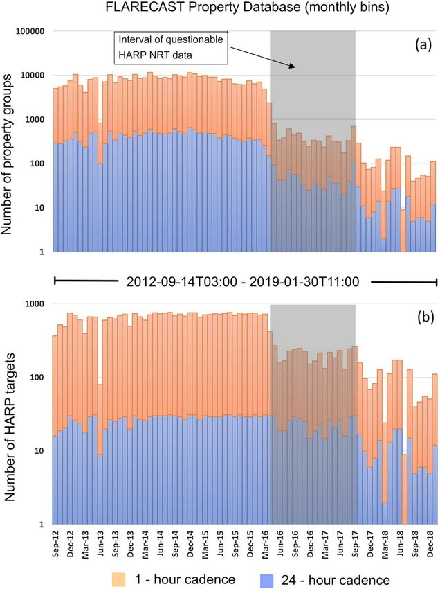
M.K. Georgoulis et al.: J. Space Weather Space Clim. 2021, 11, 39

1980s, there have been persistent efforts toward flare prediction        occurred in its course. Section 2 describes the methodology
introducing a wealth of physical, semi-empirical or empirical           followed throughout the project, while Section 3 elaborates on
AR properties and proxies that have been claimed to hold a              the tasks of data handling and monitoring. Section 4 discusses
flare-predictive capability. A short, non-exhaustive review of           the FLARECAST performance verification strategy, while
these properties, including an effort to group them into different      Section 5 briefly describes the project’s scientific results and
categories, appears in Georgoulis (2012).                               explorative component. Section 6 encapsulates the main conclu-
     However, earlier efforts (e.g., Leka & Barnes, 2003b, 2007;        sions of the project’s three top-level objectives (i.e., science,
Barnes & Leka, 2008) aiming to assess the relative performance          operations, communication) along with lessons learned in its
of these properties indicated that, on one hand, none was solely        course. Finally, in a series of Appendices we provide detailed
capable to predict flares reliably while, on the other hand, when        instructions on accessing FLARECAST data, codes and infras-
a capability to simultaneously test multiple properties was             tructure (Appendix A), key results from the FLARECAST
achieved, the predictive information contained in the full prop-        Users Survey (Appendix B; see Sect. 2.5.1 for a relevant discus-
erty set was highly redundant. The first comparative evaluation          sion), the list of refereed publications related to or acknowledg-
of prominent flare-predictive properties and methodologies,              ing the FLARECAST project (Appendix C) and, finally, a list of
undertaken by Barnes et al. (2016), established that no single          acronyms and abbreviations used in this paper (Appendix D).
method clearly outperformed the others. This and other initial              All things considered, as commented by an attendee of one
findings (e.g., the predictive value of timeseries, previous flare        of the FLARECAST Stakeholders’ Workshops, “the real fun
history) were further solidified by collaborative work on opera-         starts now”; we expect a number of future works that will take
tional forecasts by Leka et al. (2019a, b) and Park et al. (2020).      advantage of and exploit the FLARECAST products. These
     Meanwhile, the explosive increase in computing power               may not be restricted to flare prediction, as (i) the volume of
spearheaded critical advances in computer science, in an already        metadata provided by the processing of the NRT SHARP data
existing Big Data ecosystem facilitated by the wealth of ground-        product (Bobra et al., 2014) is substantial and (ii) as per EU’s
and space-based solar observations since the mid-1990s. Data            OpenAIRE initiative (https://www.openaire.eu), all data, codes
mining and the advent of machine learning eventually led to             and infrastructure of the project are openly available to any
the first application of a SVM and neural networks in flare fore-         interested individual or team worldwide. Ideally, then, one
casting (Qahwaji & Colak, 2007). Several seminal works fol-             might view the FLARECAST infrastructure as a vehicle for a
lowed thereafter (Li et al., 2008; Qahwaji et al., 2008; Song           future integrated space weather prediction platform. Compre-
et al., 2009; Yu et al., 2009; Bobra & Couvidat, 2015;                  hensive and diverse material on the FLARECAST project can
Muranushi et al., 2015; Nishizuka et al., 2017) and the list is         be found in the openly accessible FLARECAST website
ever-expanding. Today, we know that solar flare forecasting –            http://flarecast.eu (see also Fig. 9 in Sect. 2.5 for a top-level
and space weather forecasting, in general – should be viewed            structure of this website).
as an interdisciplinary effort, with a potentially critical contribu-
tion from machine learning (Camporeale et al., 2018, and refer-
ences therein), albeit not without open challenges impeding             2 The FLARECAST approach
progress (Camporeale, 2019).
     In this continuously and rapidly evolving landscape, a                 FLARECAST embraced the technical architecture and
Consortium of nine institutes spanning over six European coun-          methodology structure illustrated in Figure 2. This was realized
tries took advantage of the EU Horizon-2020 2014 PROTEC-                in a sequence of four procedural steps, namely, (1) [external]
2014 opportunity to propose the FLARECAST project. Having               data acquisition, (2) property extraction, (3) machine learning-
all the above in mind, FLARECAST pledged to develop an                  based prediction and (4) forecast verification. The overall pro-
advanced solar flare prediction system based on automatically            ject methodology was implemented in seven WPs, as follows:
extracted physical properties of solar active regions, coupled
with state-of-the-art machine learning solar flare prediction            – WP1: Project Management.
methods and validated using the most appropriate forecast               – WP2: Active Region Properties as Predictors of Flaring
verification measures. FLARECAST featured three top-level                  Activity.
objectives, namely, one scientific, one devoted to the R2O               – WP3: Flare Prediction Algorithms.
philosophy and one engaging in communication. In particular,            – WP4: Data Storage and Processing Cloud.
FLARECAST proposed:                                                     – WP5: Data and Forecast Verification.
                                                                        – WP6: Explorative Research.
– In terms of science, to understand the drivers of solar flare          – WP7: Dissemination.
  activity and improve flare forecasting.
– In terms of R2O, to provide a globally accessible flare fore-
  cast service that facilitates expansion.                                  This work plan structure, together with the technical scheme
– In terms of communication, to engage with space weather               of Figure 2, show the design philosophy of the FLARECAST
  end users, inform stakeholders and policy makers, and edu-            science and technology. The project relied on machine learning
  cate the broader public on solar flares and space weather in           applied to data from the HMI vector magnetograph (Scherrer
  general.                                                              et al., 2012; Schou et al., 2012) onboard the SDO mission
                                                                        (Pesnell et al., 2012) in order to implement a technological
    This collective work summarizes FLARECAST’s most sig-               service for flare forecasting with the ultimate goal of contribut-
nificant findings and conclusions in all three objectives above,          ing to a data-driven understanding of the physical trigger-
along with key elements from peer-reviewed publications that            ing fmechanisms of flares. Rigorous forecast verification and

                                                                Page 4 of 37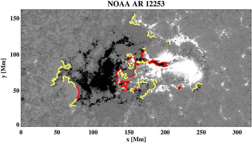
M.K. Georgoulis et al.: J. Space Weather Space Clim. 2021, 11, 39

Fig. 2. The FLARECAST architecture and WP Assignment. Rectangles indicate exchangeable software components, such as algorithms and
codes, while cylinders indicate data model components. WPs 6 and 7 are not included here but are integral to the project and complement the
overall efforts.

dissemination of results have been crucial steps of this basic         ~0.005 for GOES X5.0 flares. The climatology of the FLAR-
research effort.                                                       ECAST flare sample in the even weaker Solar Cycle 24 is 1
                                                                       GOES C-class flare every ~11 h, 1 M-class flare every ~4.5
2.1 Science motivation                                                 days and 1 X-class flare every ~67 days; substantial variations
                                                                       obviously exist over different phases of the cycle. Class imbal-
     The solar flare phenomenon pertains to explosive energy            ance in major flare prediction and other rare-event problems is a
release in the low solar atmosphere that results in short-lasting      central concern (Woodcock, 1976; Bloomfield et al., 2012;
(i.e., minutes to hours) enhancement of emission over virtually        Jolliffe & Stephenson, 2012; Bobra & Couvidat, 2015) for
the entire electromagnetic spectrum (see, e.g., Benz, 2008;            machine learning methods with proposed remedies including
Fletcher et al., 2011 for comprehensive reviews). Major,               undersampling, oversampling and misclassification weighting
highly-energetic flares (i.e., GOES M- and X-class events, in           (e.g., Longadge & Dongre, 2013; Ahmadzadeh et al., 2021).
particular) are much less frequent (in a distribution that is long          Flares at the top end of the observed energy distribution are
known to be a power law – see Drake, 1971; Rosner & Vaiana,            viewed and treated as extreme events, given their very signifi-
1978; Crosby et al., 1993) than minor flares (i.e, GOES C-class)        cant disruptive ability on top of their scarcity. For diverse
and subflares5. In terms of mean occurrence frequency, or               accounts of extreme events in physical systems one may review
climatology in the statistical language of forecasting problems        Albeverio et al. (2006), Meyers (2011) and Sharma et al.
(e.g., Barnes et al., 2016; Leka et al., 2019a), major flares fall      (2012), among other comprehensive works. These accounts also
under the category of rare events, namely, events that are much        refer extensively to two intrinsic characteristics of extreme
more infrequent than the physical systems in which they appear         events: environmental complexity and difficulty in forecasting.
(in this case, solar ARs). A typical 11-year sunspot cycle             It is a fact that forecasting solar flares is a pressing issue for
involves the appearance, evolution and fading of a few thousand        space-faring nations, mainly for two reasons: first, because of
NOAA-numbered ARs, yet Carrington’s flare is considered a               flares’ biological and technological repercussions and, second,
one-in-a-century (or even more rare) event. In other words,            because flares are a common element of the two other aspects
viewing a set of flaring ARs as a “positive” sample vs. a “neg-         of extreme space weather, CMEs and SEPs. Notwithstanding
ative” sample of non-flaring ones, the ratio of sample sizes is         the lack of an early warning for flares, mentioned already, just
substantially different than one. Increasing the flare magnitude        a cursory examination of some biological implications indicates
threshold between positive and negative samples only pushes            that, say, a 500 keV c-ray photon has a wavelength of ~0.25
this ratio to further extremes. For example, in Solar Cycle 23         nm. This is much shorter than a DNA helix (~3.5 nm), meaning
only ~1.8% of ARs hosted at least one GOES X-class flare                that such radiation acting on exposed humans engaging in
(an imbalance ratio of ~0.0183), with a respective ratio of            extravehicular activities can lead to acute radiation sickness, if
                                                                       not being altogether fatal (see, for example, Freese et al., 2016).
5
  For a definition of NOAA/GOES flare classes, see https://www.             The complexity, in terms of the multiscale (i.e., multifractal)
swpc.noaa.gov/phenomena/solar-flares-radio-blackouts.                  behavior in the turbulent solar atmosphere (see, for example,

                                                               Page 5 of 37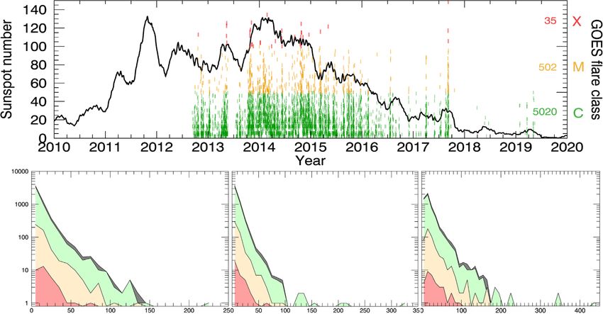
M.K. Georgoulis et al.: J. Space Weather Space Clim. 2021, 11, 39
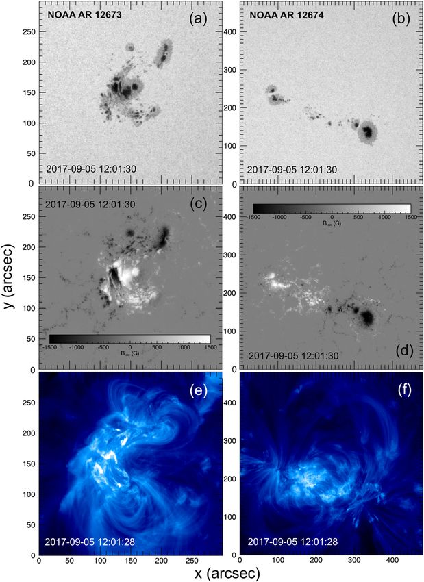
Fig. 3. Examples of two solar ARs, in terms of their photospheric continuum intensity images (a, b), LOS magnetograms (c, d) and EUV
coronal images at 19.3 nm (e, f). Both active regions were observed on 5 September 2017 at around 12:01 UT. Of them, NOAA AR 12673 (left
column) was intensely eruptive, giving the largest eruptive flares since January 2005, while NOAA AR 12674 (right column) did not host any
major flares. Images (a–d) have been acquired by HMI, while images (e, f) by AIA, both onboard the SDO mission.
Georgoulis, 2005) undoubtedly adds to the difficulty of predict- stochasticity in flare occurrence; this translates to an intrinsically
ing solar flares. In particular, flares are long thought to be probabilistic forecasting relying by definition on small probabil-
responses of nonlinear dynamical systems (solar ARs) in a ities for major and extreme flares. Randomly driven SOC mod-
SOC state. The SOC concept was initiated by seminal works els explore precisely this stochasticity; hence they are incapable
on the topic (Lu & Hamilton, 1991; Lu et al., 1993; Vlahos of predicting small- and mid-size flares. However, Strugarek &
et al., 1995) inspired by groundbreaking developments in theo- Charbonneau (2014) reported that a class of deterministically
retical physics (Bak et al., 1987, 1988; Kadanoff et al., 1989; driven SOC models could be used for predictive purposes as
see also Bak, 1996 for an encompassing account). An account they raise the memory of the system, thus exerting a partial con-
of apparent SOC manifestations in Astrophysics, including trol over flare waiting times; however, this is an avenue of
flares, is presented in relatively recent anniversary works research yet to be sufficiently explored. Recent studies have also
(Aschwanden et al., 2016; McAteer et al., 2016). However, a aimed to assess the frequency of a Carrington-level event in the
SOC evolution of flaring ARs would lead to an intrinsic framework of extreme value theory (Elvidge & Angling, 2018).
Page 6 of 37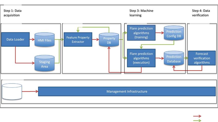
M.K. Georgoulis et al.: J. Space Weather Space Clim. 2021, 11, 39

Rather than focusing exclusively on extreme events, the key
scientific question and incentive behind the FLARECAST
project was to determine to what extent can the skill currently
achieved in the forecasting of solar flares be advanced.
    Correlating solar flares with magnetic evolution dates back
several decades. One of the earliest, pioneering accounts was that
of Howard & Severny (1963), who reported major magnetic
field changes before and after a major (coined as “great”) flare.
More systematic works were added in the 1980s with limited-
resolution magnetograms (Krall et al., 1982; Hagyard et al.,
1984; Zirin & Liggett, 1987) linking flares –and even repeated
flaring– to d-sunspot complexes and velocity shear, before the
first semi-operational flare prediction schemes appeared
(McIntosh, 1990; Zirin & Marquette, 1991). In more recent              Fig. 4. Automated PIL identification in a photospheric longitudinal
years, however, the formation of long and intense magnetic PILs        magnetogram of NOAA 12253, observed by SDO/HMI on 2 January
in the photospheric magnetic field of ARs was established as a          2015. The identified PILs in the region are further characterized as
feature of direct relevance to major flaring (for comprehensive         “moderate” (yellow contours) and “strong” (red contours). The
reviews, see Schrijver, 2009; Toriumi & Wang, 2019). By                difference between “strong” and “moderate” PILs relies on the
“intense”, we mean PILs exhibiting substantial amounts of mag-         absolute value of the gradient of the vertical magnetic field (>40 G/
netic flux and strong magnetic gradients due to the closely             pixel and >16 G/pixel, respectively) and the strength of the horizontal
seated, opposite magnetic polarities and magnetic/velocity shear       field (>120 G and >100 G, respectively). Parts of the PIL that are not
(e.g., Georgoulis et al., 2019; Patsourakos et al., 2020, and refer-   highlighted in color are below one or both thresholds and are
ences therein). Major flares occur as such PILs evolve and inten-       considered as “weak”. The algorithm used is the FLARECAST PIL
sify, fueled by magnetic flux emergence and cancellation along          identification code, accessible as described in Appendix A.2.
them (van Ballegooijen & Martens, 1989; Gibson & Fan, 2006;
Archontis & Török, 2008). Sometimes, an eruption including a
major flare may occur in the absence of intense PILs, when              magnetic fields are parameterized in order to identify and quan-
the emerging flux reconnects with the pre-existing field or has          tify patterns potentially associated with flares. Should a flare
enough magnetic twist to become unstable during emergence.             occur, flare detection and classification is primarily done using
Such a exceptional case, giving rise to a GOES X3 flare, was            the GOES 0.1–0.8 nm soft X-ray band. The peak photon flux in
reported by Gary & Moore (2004). Regardless, the majority of           this band is historically used to determine the GOES flare class.
X-class flares –the ones mostly affecting space weather condi-          There are obviously other sophisticated ways to detect flares in
                                                                       EUV, X-ray, and optical wavelengths (see Martens et al., 2012,
tions– occur above evolving, intense photospheric PILs.
                                                                       for an attempt in the framework of the HEK project), but the
    An example of ARs with and without strong PILs is given
                                                                       GOES X-ray classification is the one used most widely by the
in Figure 3, where the relatively flare-quiet (up to mid-C-class
                                                                       space weather and flare forecasting communities. Although
flares) NOAA AR 12674 is compared against the intensely
                                                                       the GOES soft X-ray detectors are, in essence, spectral irradi-
flaring NOAA AR 12673. The latter in September 6 and 10
                                                                       ance instruments without spatial resolution on the solar disk,
2017 gave the strongest (~X10) flares of solar cycle 24 (e.g.,
                                                                       observations by the GOES/SXI telescopes complement flare
Yan et al., 2018). Both active regions evolved simultaneously
                                                                       information with the source ARs, at least for the largest events.
in the solar disk, located just a few hundred arcsec away from
                                                                       However, these spatial identifications are not error-free and ver-
each other. While the photospheric compactness and conspicu-
                                                                       ification of all GOES flare locations is a nontrivial task. Signif-
ous PILs are evident in NOAA AR 12673, NOAA AR 12674 is
                                                                       icant effort on identified flare locations was also put by Hock
much more scattered. Coronal information in Figure 3 (sampled
                                                                       (2012) and, more recently, by Angryk et al. (2020).
indicatively at 19.3 nm to showcase some structure) indeed
                                                                            Quantitative active region photospheric properties, used as
shows significant complexity in terms of several bright kernels,
                                                                       flare predictors in FLARECAST’s framework, were derived from
complexity and apparent twist; significant non-potentiality, in
                                                                       the HMI SHARP data product (Bobra et al., 2014; Hoeksema
brief (e.g., Schrijver et al., 2005). Emission generally lacks
                                                                       et al., 2014). A FLARECAST processing pipeline was developed
bright kernels and does not show such non-potentiality in
                                                                       using the hmi.sharp_cea_720s_nrt data series that
NOAA AR 12674.
                                                                       contains AR maps of the LOS magnetic field component, BLOS,
    Figure 4 further shows a PIL analysis on NOAA AR 12253,
                                                                       continuum intensity, Ic, and vector magnetic field components
achieved in FLARECAST’s framework. More information is
                                                                       in the radial, Br, co-latitude, Bh, and azimuthal, B/, directions
given in Section 5.1.
                                                                       of the solar spherical coordinate system. These maps are
                                                                       produced at HMI’s JSOC6 at a cadence of 12 min, while the
2.2 Data                                                               NRT HMI stream assures that these data products are available
                                                                       within typically 4 h of acquisition7 (Hoeksema et al., 2014).
2.2.1 Active region properties and flare predictors
                                                                       6
                                                                         http://jsoc.stanford.edu/ajax/lookdata.html?ds=hmi.sharp_720s_nrt
    Flare forecasting relies almost entirely on statistical correla-   7
                                                                         This time has been varying for different intervals of the SDO
tions between solar magnetic field data and observed flare char-         mission. With the current NRT data level, data are made available
acteristics. In this case, local (i.e., AR scale) photospheric         typically within 3 h.

                                                               Page 7 of 37
M.K. Georgoulis et al.: J. Space Weather Space Clim. 2021, 11, 39

Table 1. The complete list of FLARECAST properties, separated in property groups and accounting for a total of 209 predictors. The vast
majority (197) of them correspond to the AR magnetic field, while the rest include information from the NOAA SWPC Catalogues and from
photospheric intensity images.

Data Source                 Property group            No. of     Relevant                          Adapted                  Related
                                                      predictors predictor                         from                     references
SWPC                        Solar region summary      2           McIntosh and Hale classes        McCloskey et al.         McIntosh (1990)
                            (SRS) properties                                                       (2016)
                                                      3           Number, area and                                          Lee et al. (2012)
                                                                  longitudinal extend of
                                                                  sunspots
Catalogues                  GOES soft X-ray flare 4                Flare magnitude, start, peak,
                            eventsa,b                             and end times
Surface-normal              Effective connected      1            Beff                             Georgoulis & Rust
component (radial           magnetic field                                                          (2007), Georgoulis
and line-of-sight)          strengthc                                                              (2011, 2013)
magnetograms                Fractal and multifractal 1            Fractal dimension                Conlon et al. (2008)     Abramenko et al.
                            parameters                                                                                      (2003)
                                                     1            Generalized correlation                                   Abramenko (2005)
                                                                  dimension
                                                      2           Holder exponent; Hausdorff                                Al-Ghraibah et al.
                                                                  dimension                                                 (2015)
                                                      2           Structure function’s inertial
                                                                  range index
                            Fourier and Wavelet       2           Power-law exponent             Hewett et al. (2008),
                            power spectral indices                                               Guerra et al. (2015)
                            Decay index (DI)d         8           Mean DI over PIL segments; Liu (2008)
                                                                  height of DI; ratio of PIL     Zuccarello et al. (2014)
                                                                  length to DI height
                            Magnetic PIL              5           Sum of PIL segments, longest Mason & Hoeksema
                            properties                            PIL segment                    (2010)
                                                      1           R value                        Schrijver (2007)
                                                      1           WLsg                           Falconer et al. (2012)
                            3D magnetic null          6           Number of null points in       Haynes & Parnell           Pontin et al. (2013)
                            pointsd                               different height ranges        (2007)
                                                                  (from 2 to 100 Mm above                                   Barnes & Leka
                                                                  photosphere)                                              (2006)
                            Ising Energyc             6           Original and partitioned Ising Ahmed et al. (2010)        Kontogiannis et al.
                                                                  energy                                                    (2018)
                            Magnetic energy and       11          Poynting flux and magnetic      Park et al. (2010)
                            helicity                              helicity flux proxies           Park et al. (2012)
Full-vector                 SHARP propertiese         100         Horizontal gradient of B       Bobra et al. (2014)
magnetograms                                                      components; shear angle;       (validated)
                                                                  unsigned vertical current;     Leka & Barnes (2003b,
                                                                  higher-order moments           2007)
                                                                  of time series
                            Magnetic energy and       22          Poynting flux and magnetic      Kusano et al. (2002)        Berger & Field
                            helicity                              helicity flux                                              (1984), Welsch
                                                                                                                            et al. (2009)
                            Non-neutralized           6           Total non-neutralized current Georgoulis et al.           Kontogiannis et al.
                            currents                                                            (2012)                      (2017)
                            Flows around PIL          22          Speed of                      Park et al. (2018)          Deng et al. (2006),
                                                                  diverging/converging/shear                                Wang et al. (2014)
                                                                  flows
Intensity imagesf            Magnetic field gradient 3             Total horizontal magnetic     Korsós et al. (2014)        Kontogiannis et al.
                                                                  gradient                                                  (2018)

a
  AR coronal information.
b
  The project uses the flare attributes as properties. At least one flare of desired magnitude in the forecast window signifies a positive instance.
c
  Photospheric proxy for coronal information.
d
  Uses PFEs.
e
  Most SHARP parameters correspond to mean values. In the FLARECAST pipeline, other relevant magnetogram-related parameters are also
used as predictors; these are maximum and minimum values, median, standard deviation, kurtosis, and skewness.
f
  Used in conjunction with magnetograms to calculate the sum of the magnetic field gradients between all possible opposite-polarity umbrae
pairs.

                                                                 Page 8 of 37
M.K. Georgoulis et al.: J. Space Weather Space Clim. 2021, 11, 39

Fig. 5. Monthly numbers of (a) calculated property groups and (b) processed NRT SHARP timestamps between 14 September 2012 and 30
January 2019. Property group numbers are shown at highest (1-h; orange bars) and at lowest (24-h; blue bars) cadence. The shaded interval
between 13 April 2016 and 8 September 2017 corresponds to a period of questionable quality for the HMI NRT SHARP data (see text for
details). Histograms represent a total of 32,098 processed SHARP timestamps, leading to millions of predictor values, since each timestamp
could potentially provide up to 209 predictors.

Another reason for using the NRT stream was that any                      In the FLARECAST processing pipeline, NRT SHARP
operationally-oriented flare forecasting service has to rely on         maps are pre-processed before extracting any property. Pre-
NRT data for training, testing, and validation of its method(s).       processing aims to:
In a further attempt to replicate operational conditions to the
greatest extent possible, FLARECAST did not restrict its input         (a) check for missing information in the FITS headers and
data to longitudinal areas close to the central solar meridian,            restore it, if possible;
but identically treated all data regardless of solar disk position     (b) examine for bad-quality or missing data (i.e., a NaN or a
(for regions very close to the solar limbs though, some selection          constant value);
criteria were imposed, as discussed below). This was decided in        (c) capture possible differences between WCS (Thompson,
spite of a complete understanding that magnetic projection                 2006) positions and header positions;
effects, foreshortening and noise near the solar limbs are             (d) trim any part of the FOV containing off-disk pixels for
substantial.                                                               ARs near the limbs.

                                                              Page 9 of 37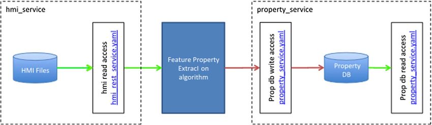
M.K. Georgoulis et al.: J. Space Weather Space Clim. 2021, 11, 39

Fig. 6. Attributes of 5557 SHARP-associated flares over September 2012 to May 2019. (a) Flare onset times, in terms of GOES classes X (red),
M (orange) and C (green) and respective sub-classes (tick marks; right ordinate), plotted over the 90-day averaged sunspot number over Solar
Cycle 24 (left ordinate; Source: Sunspot Index and Long-Term Solar Observations [SILSO], Royal Observatory of Belgium). The numbers of
flares for each GOES class are also given. The bottom line shows waterfall diagrams of the distributions of rise time (b), decay time (c) and
duration (d). Extrema for each distributions are shown in each plot. The “All flares” diagram corresponds to the sum of flare numbers in each
bin. We use fixed, 10-min bin sizes.

     Magnetogram maps are flagged as null and no properties are          however, as per the sensitivity analysis of Section 4.3. Evaluat-
calculated for HARP timestamps and dates with (i) bad-quality           ing the impact of predictor uncertainties in multi-parametric
data, (ii) absolute differences between FITS header coordi-             machine learning prediction schemes could be a meaningful
nates and WCS-calculated coordinates that are larger than 5 or         future step.
(iii) trimmed images that are less than 20 pixels in horizontal size.       Up to 209 predictors are calculated from each SHARP
     Active region properties extracted from the photospheric           observation at different cadence, namely 1 h, 3 h, 6 h, 12 h,
magnetic field in FLARECAST have all been previously                     and 24 h. The full 12-min cadence of HMI SHARPs was
tested for relevance in flare prediction. These properties are           exploited only in a very limited number of cases, due to the
presented in Table 1, itemized into 15 different groups. Each           immense computational time it required. This computational
property group relates to either a certain property or a set of         expense dictated the different cadence as a necessity. Clearly,
properties and gives rise to one or more flare predictors, respec-       FLARECAST did not restrict to the 25 scalar properties
tively. These predictors, and groups thereof, quantify the state of     included in the SHARP predictor metadata. It did, however,
the AR photosphere and corona and reflect (1) the entire region          replicate the calculations of these predictors to validate them
or SHARP FOV, (2) magnetic PILs, or (3) sunspots (as the                and consider additional image statistics (i.e., higher-order
areas with the strongest magnetic field). Most property groups           moments). Instructions on how to access these and other data
characterise only the state of the photospheric magnetic field.          and information are detailed in Appendix A.
Some, however, characterize the state of the AR corona, either              Figure 5 displays histograms of the monthly number of prop-
by photospheric proxies or by means of current-free PFEs or             erty groups and SHARP timestamps analyzed over the period
by differences between the photospheric field and that expected          September 2012 – January 2019, for the finest (1 h) and the
by a PFE. The two last columns of Table 1 indicate relevant             coarsest (24 h) cadences considered. Numbers corresponding
published work, distinguishing between studies that were                to 12-min cadence are not shown due to their lack of statistical
directly implemented in the course of the project from additional       significance. The progression of Solar Cycle 24 can be roughly
or previous studies pertinent to some predictors.                       assessed, with significantly higher numbers until early 2016,
     It should be mentioned that, for many of the properties in         when the declining phase gave way to the latest solar minimum.
Table 1, estimating uncertainties is nontrivial. For the cases          Thereafter, the numbers of both calculated property groups and
uncertainties exist, mostly in terms of r-values in fits, these          processed SHARP timestamps gradually decline as eligible
values are provided in the property database. This said, predic-        SHARPs in the NRT stream become fewer and fewer. The
tion algorithms (Sect. 2.3) currently do not utilize predictor          shaded interval between 13 April 2016 and 1 September 2017
uncertainties. Uncertainties in verification metrics are provided,       corresponds to a time of potentially problematic NRT data due

                                                                Page 10 of 37
M.K. Georgoulis et al.: J. Space Weather Space Clim. 2021, 11, 39
Table 2. FLARECAST unsupervised and supervised machine 2. If any NOAA ARs are assigned to the SHARP, the SWPC
learning methods (final release). flare event list is searched for those NOAA numbers and
related flares are associated to all of that SHARP’s prop-
Unsupervised methods – K-means
erty database entries.
– Fuzzy C-means
– Possibilistic C-means 3. For X-ray flares with no reported NOAA number, loca-
tions of co-temporal flares observed in ground-based Ha
Supervised methods – LASSO images (also from the NOAA/SWPC flare event list) are
– Hybrid LASSO used to determine if the multi-wavelength flare event
– Elastic net occurred within the SHARP’s FOV (again taking solar
– Logit
– Hybrid Logit
differential rotation into account). Positive Ha flare asso-
– Random forests (RFs) ciation results in the inclusion of the respective X-ray
– Multi-layer perceptron (MLP) flare. A very small fraction of flares of GOES class C
– Recurrent neural network (RNN) and above, of the order 0.1%, seems to miss both criteria
– Support vector machine (SVM) above over the analysis period.
– Garson’s method
– Olden’s method After all SHARP-associated flares are identified, we extract
the following properties for each flare:
– FM: GOES peak magnitude (e.g., M1.3).
– ss: Time difference (in seconds) between the SHARP
to a transient misalignment between the two HMI cameras pro- observation time T0 and the reported flare start time Ts (i.
viding filtergrams for the generation of the full Stokes vector8. e., ss = Ts T0).
Only definitive vector magnetogram data were reprocessed – – sp: Time difference (in seconds) between T0 and the
NRTs were not – while full-disk LOS magnetograms at 45s reported flare peak time Tp (i.e., sp = Tp T0).
cadence were not affected. Artifacts in this case intensify with – se: Time difference (in seconds) between T0 and the
increasing central meridian distance. reported flare end time Te (i.e., se = Te T0).
The property data set shown in Figure 5 is, to our knowledge
and understanding, one of the largest and most diverse ever Figure 6 provides a snapshot of FLARECAST’s flare data
assembled for flare prediction, offering unique opportunities set and displays the temporal distribution of different flare
for statistical and physics-based studies to interested teams classes for Solar Cycle 24 (Fig. 6a), along with their rise time
worldwide. In Guerra et al. (2018), a sub-group of six predictors (Fig. 6b), decay time (Fig. 6c) and duration (Fig. 6d) for approx-
were studied to determine the effects of using the LOS field imately the same time coverage as that of the property database
(BLOS) versus the surface-radial field (Br) for their calculation statistics in Figure 5. Rise/decay times and durations have been
and subsequent use in flare forecasting. It was determined that provided by NOAA.
both LOS and radial field components can be advantageous in We consider as eligible flares only those of GOES C-class
different circumstances. The project hence decided to use both and above (i.e., C1.0) to make sure that as many as possible
property versions to facilitate any independent information these are included, unobscured by an often elevated solar soft X-ray
two versions could furnish. background. We acknowledge, though, that even a C1.0 flare
threshold might result in loss of some flares in cases of intensely
2.2.2 Flare association high solar activity. Others may be lost due to lack of, or an
erroneous, location information.
The NOAA/SWPC flare event list data include the universal
times (UT) of their start (i.e., onset), peak, and end, along with 2.3 Methods: machine learning
the flare magnitude, all obtained by the GOES spacecraft 0.1–
0.8 nm soft X-ray channel. Where possible, source ARs are The FLARECAST computational component fully relied on
identified from the daily NOAA/SWPC flare event lists, with machine learning, that is, on prediction algorithms that utilize an
their morphological properties extracted from the daily automatic learning step based on either labeled or unlabeled
NOAA/SWPC SRS reports. NOAA ARs, flaring or not, are input data. The conceptual core of each machine learning tech-
linked to the HMI SHARPs and the FLARECAST property nique lies on the modality of this learning step. Labeled data are
database includes information on all ARs located within each characterized by a tag including one or more property-specific
SHARP FOV. labels (e.g., flaring or non-flaring), whereas unlabeled data are
The process below is followed for each SHARP during its free of such tags.
solar disk passage: We distinguish between two broad categories of relevant
machine learning methods:
1. SHARPs are first checked to determine whether their
FOV contains the time-advanced centroid locations of – Unsupervised methods, that are free to infer the data struc-
NOAA-numbered ARs. This makes use of the closest ture from the data themselves and realize the learning task
SRS report before the SHARP observation, with solar in a fully data-driven manner. Such methods train on unla-
fdifferential rotation taken into account. beled data.
– Supervised methods, that perform an unknown input-output
8 mapping from known input–output samples. Sparsity
See https://solarnews.nso.edu/20170901/#section_hoeksema for
more information. enhancing techniques in these methods enable a quantitative
Page 11 of 37M.K. Georgoulis et al.: J. Space Weather Space Clim. 2021, 11, 39
ranking of properties (predictors) that contribute most to the Benvenuto et al., 2018; Florios et al., 2018). A detailed descrip-
achieved prediction. Supervised methods nominally train on tion of these methods is beyond the scope of this work. The latest
labeled data. release of the project’s platform contains a standard MLP trained
by means of Error-Back-Propagation and two RNNs that allow
The project’s machine learning inventory comprises three feedback loops in the feed-forward architecture. This modifica-
(3) unsupervised and eleven (11) supervised machine learning tion is realized by means of both an Elman neural network
methods, listed in Table 2. We chose to implement a diverse (Elman, 1990), in which any number of context nodes is permit-
array of methods because we identified a need to experimentally ted, and a Jordan neural network (Jordan, 1997) serial, in which
test the strengths and weaknesses of each method, along with the number of context nodes is constrained to coincide with the
their key differences and predictive capacity. Identifying the number of output nodes.
state-of-the-art in machine learning methods flows directly from In a more recent development, regularization neural net-
FLARECAST’s main goal (Sect. 1). works (Evgeniou et al., 2000) enable the connection between
training and generalization via the minimization of functionals
2.3.1 Unsupervised methods such as the following,
FLARECAST proposes three unsupervised (i.e., clustering) V ðy i ; f ðxi ÞÞ þ kf F ! minimum; ð4Þ
methods for the automatic classification of sets of unlabeled AR where fðxi ; yi Þgi¼1
N
represents the training set made of N prop-
properties. To briefly explain how these three algorithms work, erty-label pairs, V(,) is the loss function that measures the
we denote as X ¼ fxk jxk 2 Rd k ¼ 1; . . . ; ng a set of unlabeled price paid for the inaccuracy of predicting yi with f(xi), and
samples xk = (x1k, . . . , xdk), where xik is the i-th property of the k is the regularization parameter, which realizes the trade-
k-th sample xk, d is the dimension of the property space Rd and off between fitting over the training set and generalization.
Y ¼ fy j jy j 2 Rd ; j ¼ 1; . . . ; cg is the set of the c centers of the SVM for regression (Scholkopf & Smola, 2001) is one of the
clusters to determine. The algorithms’ objective is to minimize a standard regularization networks implemented in FLARECAST.
certain functional with respect to the cluster centers. The func- In this case, V(,) is a standard quadratic loss function and F is a
tionals of the K-means (Anderberg, 2014) and Fuzzy C-means Reproducing Kernel Hilbert Space (De Vito et al., 2004), in
(Bezdek, 1981) algorithms are given by, which four different kernel types can be selected (i.e., linear,
X n X c polynomial, radial basis function, and sigmoidal). The FLARE-
J ðX ; Y ; U Þ ¼ ujk d2jk ; ð1Þ CAST platform also contains a SVM for classification that uses
k¼1 j¼1 the hinge loss function, namely the one thought most appropriate
and, for classification (Rosasco et al., 2004). Two sparsity enhancing
n X
X c regularization methods were also implemented, in which the
J m ðX ; Y ; U Þ ¼ ðujk Þm d2jk ; ð2Þ number of features that effectively contribute to the generaliza-
k¼1 j¼1 tion is constrained to the smallest possible. This is achieved by
minimizing the l1 norm of the feature vector (i.e., the sum of
respectively. In both equations above, U = [ujk] is the n c the absolute values of its components), which is further achieved
membership matrix whose entries represent the memberships by means of two different approaches: penalized logistic regres-
of the k-th sample to the j-th cluster and djk is the distance of sion (Wu et al., 2009), in which the loss function realizes the
the k-th sample from the j-th cluster center. In the case of the Bernoulli distribution for the labels, and LASSO (Yuan & Lin,
K-means algorithm, the memberships are binary values, while 2006), in which the loss function is quadratic. FLARECAST
in the case of the Fuzzy C-means algorithm they are real num- also includes a hybrid version of penalized logistic regression
bers 2[0, 1], representing the membership probability. In the and LASSO, in which the regression outcome is partitioned by
latter case, there is also a “fuzzifier” parameter m. means of a Fuzzy C-means scheme, without focusing on opti-
The third clustering method is Possibilistic C-means mizing a specific skill score (Benvenuto et al., 2018). The plat-
(Krishnapuram & Keller, 1996; Massone et al., 2006). This is form contains a further generalization, namely an elastic net
an elaborate development of Fuzzy C-means, in which each (Zou & Hastie, 2005) algorithm, in which the minimization
sample can, in principle, belong simultaneously to several clus- functional contains two penalty terms (l1 and l2) with two differ-
ters with different degrees of membership. In this case the cost ent regularization parameters optimized by cross validation.
function to minimize is given by, Ensemble learning (Dietterich, 2000) is another supervised
n X
X c X
c X
n
m
approach that uses a combination of different learning models
J m ðX ; Y ; U Þ ¼ ðumjk d2jk Þ þ gj ð1 ujk Þ ; ð3Þ to increase the classification accuracy. In this framework,
k¼1 j¼1 j¼1 k¼1 FLARECAST offers a RF algorithm (Breiman, 2001), which
where the entries of the membership matrix satisfy the con- works as a large collection of de-correlated decision trees. Given
straint maxjujk > 0 "k and, for each j, the regularization a training set of samples made of properties and corresponding
parameter gj depends on the average size and shape of the labels, a decision tree recursively splits the training samples into
j-th cluster. subsets based on the value of a single property. Each split cor-
responds to a node in the tree and the task is to separate records
2.3.2 Supervised methods in the training set that have different characteristics. We follow
the implementation described in Liaw & Wiener (2002), by
Most FLARECAST methods are supervised, in line with splitting the tree until every subset is pure (i.e., all samples in
contemporary applications of machine learning to flare the subset belong to the same class). In this way all terminal
prediction (e.g., Ahmed et al., 2013; Bobra & Couvidat, 2015; nodes (i.e., the leaves) are assigned a unique class label. Once
Page 12 of 37M.K. Georgoulis et al.: J. Space Weather Space Clim. 2021, 11, 39
Fig. 7. A data component (dashed box) consists of a database (blue cylinder) and a well-defined API (white box). An algorithm (blue rectangle)
uses this API to read data (green arrow) and another API to write data (red arrow) into a separate data component.
the decision tree has been constructed, classifying a test record downloaded using the SDO NetDRMS and archived as part of
is achieved by starting from the root node, applying the test con- the MEDOC solar physics data archive. Besides the one used pri-
dition to the record and following the appropriate branch based marily for the forecasting tasks (hmi.sharp_cea_720s_
on the outcome of the test. This can lead either to another inter- nrt), downloaded series included hmi.m_720s, hmi.
nal node, for which a new test condition is applied, or to a leaf m_720s_ nrt, hmi.sharp_720s, hmi.sharp_720s_
node. If a leaf node is reached, the label associated with it is nrt, hmi.sharp_cea_720s, hmi.ic_720s and hmi.
assigned to the record. In the RF approach, the training set is ic_nolimbdark_720s_nrt. Not all of them were finally
randomly divided into a fixed number of subsets and for each used by the Consortium, although definitive SHARP data and
subset a decision tree is built. New, incoming unlabeled samples continuum images were used for tasks akin to the explorative
are classified by aggregating the predictions of the decision trees science component (Sect. 5). NRT data series were downloaded
via a majority vote procedure. no later than 1 hr after they were made available by HMI’s JSOC.
Details on how to obtain the FLARECAST machine learn- This overall delay could be further reduced, if necessary, by more
ing algorithms can be found in Appendix A. We note in passing frequent download requests.
that the landscape of machine learning methods is continuously
and rapidly evolving, with new algorithms constantly intro- 2.4.3 FLARECAST software architecture
duced. Our approach, as explained in Section 2.4.3 below, is
an implementation based on modularity in such a way that The FLARECAST architecture design was driven by the
incoming machine learning methods can be easily integrated needs for modularity, portability and ability to perform and
in the FLARECAST platform. accommodate different algorithms written in various program-
ming languages. This philosophy is best described by the top-
2.4 Technology level diagram of Figure 2 in Section 2. The diagram reflects
the four processing steps of the FLARECAST pipeline:
FLARECAST relies on a broad selection of different tech-
nologies, including hardware for storage and computing as well
as software for data handling, infrastructure management and – Step 1: Acquisition and transformation of data from multi-
computation. The software was designed in a way that is hard- ple sources (SDO/HMI & NOAA SWPC – Sect. 2.2).
ware independent and can be installed on numerous platforms. – Step 2: Extraction of properties from the data by several
All code developed during FLARECAST has been published algorithms (Sect. 2.2).
under an open source license and is freely available. Code – Step 3: Prediction through implementation of several
acquisition and license information are detailed in Appendix A. machine learning algorithms (Sect. 2.3).
– Step 4: Verification of the generated forecast data products
2.4.1 Computing hardware (Sect. 4).
A computing server dedicated to FLARECAST has been The underlying management infrastructure controls and
integrated into the MEDOC computing infrastructure9 and hosts monitors these algorithms. The layout of the FLARECAST
the production version of the FLARECAST pipeline. Queries architecture simplified the project management as the individual
on this server for SDO/HMI data are made directly into the components are under the responsibility of dedicated WPs. The
MEDOC database tables, and SDO/HMI files are accessed relation between components and WPs is shown by the black
locally. This allows efficient runs of the FLARECAST property rectangles in Figure 2. The software infrastructure is discussed
extraction algorithms. in detail in Section 3.
2.4.2 Data storage hardware
2.4.4 Software components
The main FLARECAST data volume is provided by eight
SDO/HMI data series at 12 min cadence that have been The software components, represented by the blue rectan-
gles in Figure 2, fulfill specific tasks such as data loading, prop-
9
https://idoc.ias.u-psud.fr/MEDOC erty extraction, machine learning, or verification. Generally,
Page 13 of 37M.K. Georgoulis et al.: J. Space Weather Space Clim. 2021, 11, 39
Fig. 8. Components of the FLARECAST architecture within the main Docker engine. The different grayscale rectangles correspond to
different Docker containers, while adjacent containers typically share a common interface.
a software component contains several algorithms and each containers co-exist and function independently. A Docker con-
algorithm implements a specific variant of a task. Each property tainer can be viewed as a light-weight virtual machine that hosts
extraction or machine learning method, for example, has its own an arbitrarily configured software environment. This includes
dedicated algorithm. custom programming languages and different library versions
The management infrastructure orchestrates the execution of per container. Each FLARECAST infrastructure component or
the FLARECAST workflow. It launches the extraction algo- algorithm is deployed in a dedicated Docker container. These
rithms as soon as new observational data arrives. After they containers can be installed on a high performance cluster as well
are finished, the management infrastructure triggers the flare as on a developer’s desktop machine, making it possible to
prediction algorithms. deploy FLARECAST in different environments at the same
The management infrastructure is implemented as a col- time. A schematic of the FLARECAST Docker containers is
lection of containers (see Sect. 2.4.6 below). In automated shown in Figure 8.
mode, a set of repeatedly executed computer scripts (i.e., cron
jobs) regularly check for new data and start the algorithms, if 2.4.7 Language independence
necessary. Additionally, a small web application allows users
with administrator privileges to manually trigger the execution As mentioned already, algorithms may be written in any
of algorithms. programming language. This allows to re-use already existing
libraries for certain tasks. Currently tested and supported are
2.4.5 Data components Python 2.7 and 3.0, the Interactive Data Language (IDL) 8.5
and R. Other languages that can be executed on a Linux system
The blue database symbols in Figure 2 denote individual (e.g., Java, C++ and Perl) are not expected to generate major
parts of the FLARECAST data model, hereafter referred to as issues, but we must make clear that we have not systematically
data components. Within the workflow, every software compo- tested them.
nent (i.e., every algorithm) reads from several and writes to pre-
cisely one data component. Like this, the software components
are decoupled from each other and only have to provide a con- 2.4.8 Data model
trol interface (start, stop) for the management infrastructure. The
management infrastructure connects to a dedicated data compo- The design of the data model is balanced between flexible
nent for configuration and data logging. support for different kinds of data structures and strict schema
Each data component defines a generic interface to read, definitions for better interoperability. This can be achieved
create, update, and delete data. The read methods include a through a semi-structured data model. Its main structures are
query language for simple queries. Figure 7 illustrates this pro- defined by a traditional table-based, relational data model. Indi-
cess for an example property extraction algorithm. vidual entries of the table support weakly-typed data types (i.e.,
types supported by weakly- or loosely-typed programming lan-
guages, such as C). In this sense, an algorithm can handle data
2.4.6 Docker containers types as simple as numeric values or strings simultaneously with
more complex data types, such as arrays, matrices, dictionaries
All FLARECAST infrastructure components are imple- and whole hierarchies of objects. For the weakly-typed data
mented as Docker containers. Docker10 is an open source soft- types we rely on the built-in JSON data type of PostgreSQL
ware ecosystem (i.e., engine) in which different Docker 9.6. Algorithms encode their output (e.g., extracted properties)
in the JSON data format. JSON is supported by most C-like pro-
10
https://www.docker.com gramming languages, including Python, R and IDL.
Page 14 of 37You can also read