The Gaia EDR3 view of Johnson-Kron-Cousins standard stars
←
→
Page content transcription
If your browser does not render page correctly, please read the page content below
Astronomy & Astrophysics manuscript no. PhotSets                                                                                     ©ESO 2022
                                               May 13, 2022

                                                   The Gaia EDR3 view of Johnson-Kron-Cousins standard stars:
                                                           the curated Landolt and Stetson collections?
                                                   E. Pancino      1, 2 ,   P. M. Marrese   3, 2 ,
                                                                                                S. Marinoni 3, 2 , N. Sanna 1 , A. Turchi 1 , M. Tsantaki                1,   M. Rainer   1, 4 ,

                                                                                            G. Altavilla 3, 2 , M. Monelli 5, 6 , L. Monaco 7

                                                     1
                                                         INAF – Osservatorio Astrofisico di Arcetri, Largo E. Fermi 5, I-50125 Firenze, Italy
                                                     2
                                                         Space Science Data Center – ASI, Via del Politecnico SNC, I-00133 Rome, Italy
                                                     3
                                                         INAF – Osservatorio Astronomico di Roma, Via Frascati 33, I-00078, Monte Porzio Catone (RM), Italy
                                                     4
                                                         INAF – Osservatorio Astronomico di Brera, via E. Bianchi 46, I-23807 Merate (LC), Italy
arXiv:2205.06186v1 [astro-ph.SR] 12 May 2022

                                                     5
                                                         Instituto de Astrofísica de Canarias, Calle Via Lactea, E-38205 La Laguna, Tenerife, Spain
                                                     6
                                                         Facultad de Física, Universidad de La Laguna, Avda astrofíísico Fco. Sánchez s/n, E-38200 La Laguna, Tenerife, Spain
                                                     7
                                                         Departamento de Ciencias Fisicas, Universidad Andres Bello, Fernandez Concha 700, Las Condes, Santiago, Chile
                                                     Received: —

                                                                                                                  ABSTRACT

                                                     Context. In the era of large surveys and space missions, it is necessary to rely on large samples of well-characterized stars for inter-
                                                     calibrating and comparing measurements from different surveys and catalogues. Among the most employed photometric systems, the
                                                     Johnson-Kron-Cousins has been used for decades and for a large amount of important datasets.
                                                     Aims. Our goal is to profit from the Gaia EDR3 data, Gaia official cross-match algorithm, and Gaia-derived literature catalogues,
                                                     to provide a well-characterized and clean sample of secondary standards in the Johnson-Kron-Cousins system, as well as a set of
                                                     transformations between the main photometric systems and the Johnson-Kron-Cousins one.
                                                     Methods. Using Gaia as a reference, as well as data from reddening maps, spectroscopic surveys, and variable stars monitoring
                                                     surveys, we curated and characterized the widely used Landolt and Stetson collections of more than 200 000 secondary standards,
                                                     employing classical as well as machine learning techniques. In particular, our atmospheric parameters agree significantly better with
                                                     spectroscopic ones, compared to other machine learning catalogues. We also cross-matched the curated collections with the major
                                                     photometric surveys to provide a comprehensive set of reliable measurements in the most widely adopted photometric systems.
                                                     Results. We provide a curated catalogue of secondary standards in the Johnson-Kron-Cousins system that are well-measured and
                                                     as free as possible from variable and multiple sources. We characterize the collection in terms of astrophysical parameters, distance,
                                                     reddening, and radial velocity. We provide a table with the magnitudes of the secondary standards in the most widely used photometric
                                                     systems (ugriz, grizy, Gaia, Hipparcos, Tycho, 2MASS). We finally provide a set of 167 polynomial transformations, valid for dwarfs
                                                     and giants, metal-poor and metal-rich stars, to transform U BVRI magnitudes in the above photometric systems and vice-versa.
                                                     Key words. Techniques: photometric — Catalogs — Surveys — Stars: fundamental parameters

                                               1. Introduction                                                                Along the years, several photometric systems were proposed
                                                                                                                          (see Bessell 2005, for a comprehensive review), both based on
                                               The Johnson-Kron-Cousins system is one of the most widely                  wide bands and on medium or narrow bands that pinpoint im-
                                               used photometric systems over the years. It was designed build-            portant spectral features for specific research goals (for example
                                               ing on the work made previously by various researches, most                the Strömgren system: Strömgren 1966), while a large part of
                                               notably on the Johnson U BV (Johnson & Morgan 1953; John-                  the present-day photometric surveys is based on variations of the
                                               son 1963; Johnson et al. 1966), Kron RI (Kron et al. 1953)                 SDSS ugriz or the Pan-STARRS grizy systems (Fukugita et al.
                                               and Cousins VRI (Cousins 1976, 1983, 1984) photometric sys-                1996; Tonry et al. 2012, see also Section 5 and Figure 10). The
                                               tems. Indeed, the Johnson system in 1966 formed the basis of               Johnson-Kron-Cousins system is still alive and widely employed
                                               most subsequent photometric systems in the optical and near in-            today, but the fact that several other photometric systems are now
                                               frared (Bessell 2005). In 1992, Arlo U. Landolt published a com-           equally or even more widely used, imposes the need to "connect"
                                               prehensive catalogue of equatorial standard stars which, from              or "compare" measurements in different systems, if one wants to
                                               then on, became the fundamental defining set for the U BVRI                profitably use data from different sources. One particularly strik-
                                               Johnson-Kron-Cousins system, and was used in the last three                ing example is in the field of variable star studies (Monelli &
                                               decades to calibrate the vast majority of all imaging observations         Fiorentino 2022), where the use of long time series is one of the
                                               in the U BVRI passbands. The Johnson-Kron-Cousins system is                most fundamental tools, and the need of homogeneous photom-
                                               mounted on optical instruments in most of the 8 m telescopes               etry is of paramount importance. Photometric variability stud-
                                               presently available, including VLT, LBT, Subaru, or Keck.                  ies are in fact gradually moving from the Johnson-Kron-Cousins
                                                                                                                          system (for instance the OGLE or ASAS-SN surveys, Kaluzny
                                                                                                                          et al. 1995; Shappee et al. 2014) to ugriz or grizy systems (such
                                                ?
                                                   This paper is dedicated to Arlo U. Landolt, one of the fathers of      as the ZTF or the upcoming LSST, Ivezić et al. 2019; Chen et al.
                                               photometry, who passed away on 21 January 2022.

                                                                                                                                                                     Article number, page 1 of 19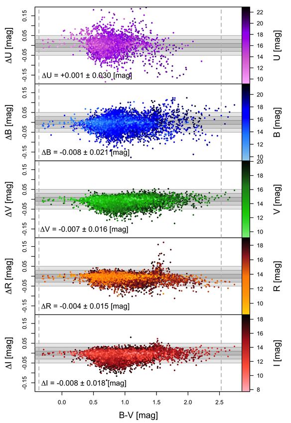
A&A proofs: manuscript no. PhotSets

Fig. 1. The V magnitude (left panels) and B-V color (right panels) dis-
tribution of the Landolt (top panels) and Stetson (bottom panels) collec-
tions. The full samples are plotted in grey, the samples with a match in
Gaia EDR3 in light colors, and the best-quality samples (see Section 4.1
for details) in full colors. The dotted vertical lines show the coverage of
the original Landolt (1992) standards set.
                                                                              Fig. 2. Distribution in RA and Dec on the sky of the Landolt (top panel)
                                                                              and Stetson (bottom panel) collections, in an Aitoff projection. Note that
                                                                              some of the Landolt fields are also included in the Stetson collection.
                                                                              The sizes of the symbols are proportional to the magnitudes and darker
                                                                              colors correspond to higher star densities.

2020) and thus there is the need to accurately and precisely con-
nect the two systems. That community has indeed started its own               2. The Landolt and Stetson collections
dedicated survey for the purpose, the AAVSO photometric all
sky survey (APASS1 , Henden et al. 2012; Levine 2017), which                  2.1. The Landolt collection
employs the B and V bands from the Johnson-Kron-Cousins sys-
                                                                              The Landolt standards (Landolt 1992) are the foundation of the
tem, together with the ugriz passbands from the SDSS system.
                                                                              Johnson-Kron-Cousins photometric system. Although they are
                                                                              tied to the Vega zero-point, they are based on the sets of pri-
    In this paper we build on the large body of exquisite mea-                mary standards in UBV by Johnson (1963) and in RI by Cousins
surements by A. U. Landolt, (Landolt & Uomoto 2007; Landolt                   (1976). In practice, they were used for three decades to calibrate
2007, 2009, 2013; Clem & Landolt 2013, 2016), P. B. Stetson                   the vast majority of all imaging observations in the U BVRI pass-
and collaborators (Stetson & Harris 1988; Stetson 2000; Stetson               bands. The original 1992 photoelectric set was later extended
et al. 2019), to provide a sample of more than 200 000 secondary              with observations far from the celestial equator and also with a
standards, accurately calibrated on the original standards by Lan-            large amount of CCD observations. We consider here a series
dolt (1992). The Landolt and Stetson collections have been cu-                of works by Landolt and collaborators, that can be divided into
rated, pruned of variable stars and binaries, and cross-matched               two subgroups: one based on photoelectric observations (Lan-
– with the help of Gaia – to several large photometric surveys                dolt 1992; Landolt & Uomoto 2007; Landolt 2007, 2009, 2013)
in different photometric systems. The two collections have also               and the other on CCD observations (Clem & Landolt 2013,
been characterized in terms of atmospheric parameters, redden-                2016). We also complement the set with U BVRI measurements
ing, distance, and therefore will hopefully enable a variety of               for two CALSPEC2 (Bohlin 2014; Bohlin et al. 2019) standards
calibration and inter-comparison tasks, including the calibration             by Bohlin & Landolt (2015). A preliminary version of the Lan-
of Johnson-Kron-Cousins measurements from images that were                    dolt collection presented here was used to validate the Gaia
not observed together with Landolt (1992) standard fields.                    Spectro-Photometric Standard Stars for the flux calibration of
                                                                              Gaia (hereafter SPSS; Pancino et al. 2012, 2021; Altavilla et al.
                                                                              2015, 2021; Marinoni et al. 2016). A more advanced preliminary
    The paper is organized as follows: in Section 2 we present                version of this collection was used to standardize the synthetic
the Landolt and the Stetson collections; in Section 3 we describe             photometry obtained from the Gaia DR3 low-resolution spectra
the cross-match with Gaia and all the quality checks on the data,             (R=λ/δλ ' 20 − 100, Gaia collaboration, Montegriffo et al., in
including the identification of binary and variable stars; in Sec-            preparation).
tion 4 we compare and combine the collections into one cata-                      When assembling the Landolt collection, we always chose
logue, and we characterize its stellar content in terms of dis-               the most recent measurement in case of stars re-observed in dif-
tance, reddening, classification, and stellar parameters; in Sec-
tion 5 we compute transformations between the Johnson-Kron-                   1
                                                                                https://www.aavso.org/apass
Cousins system and some other widely used photometric sys-                    2
                                                                                https://www.stsci.edu/hst/instrumentation/
tems; finally, in Section 6 we summarize our results and draw                 reference-data-for-calibration-and-tools/
our conclusions.                                                              astronomical-catalogs/calspec

Article number, page 2 of 19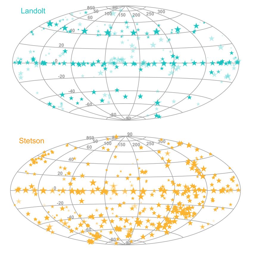
E. Pancino et al.: The Gaia view of Johnson-Kron-Cousins standards

Table 1. The curated Landolt collection (Section 2.1), with re-calibrated   uncertainties in the curated Landolt collection have been re-
uncertainties and cross-match analysis parameters (Section 3.1). This       calibrated as described in Section 3.1.
table contains also 520 stars with no Gaia EDR3 match (Section 3.1),
thus we report both the original Landolt coordinates and the Gaia EDR3
ICRS coordinates (epoch J2016), when available.                             2.2. The Stetson collection

  Column              Units     Description                                 The Stetson database3 (Stetson 2000; Stetson et al. 2019) is
  Unique ID                     Unique star ID defined here                 based on more than half a million public and proprietary CCD
  Gaia EDR3 ID                  Gaia Source ID from EDR3                    images, collected by P. B. Stetson starting in 1983, when public
  Star Name                     Landolt star name                           archives did not exist yet. The images cover open and globular
  RAorig              deg       Landolt original right ascension            clusters, dwarf galaxies, supernova remnants, and other interest-
  Decorig             deg       Landolt original declination                ing areas on the sky, including some Landolt (1992) standard
  RAEDR3              deg       Gaia EDR3 right ascension                   fields. All images were obtained in U BVRI filters and were uni-
  DecEDR3             deg       Gaia EDR3 declination                       formly processed. Photometry was derived with the DAOPHOT
  U                   mag       U-band magnitude                            package (Stetson 1987, 1994) and calibrated on the Johnson-
  σU                  mag       re-calibrated uncertainty on U              Kron-Cousins system based on repeated Landolt (1992) standard
  nU                            number of U-band measurements               field observations. It is worth noting that, unlike in the Landolt
  B                   mag       B-band magnitude                            collection, the Stetson collection measurements were obtained
  σB                  mag       re-calibrated uncertainty on B              by profile fitting, and then corrected with aperture photometry
  nB                            number of B-band measurements               curves of growth. Only stars matching strict quality criteria were
  V                   mag       V-band magnitude                            considered as secondary U BVRI standards: (i) observed at least
  σV                  mag       re-calibrated uncertainty on V              five times independently in photometric conditions, (ii) with un-
  nV                            number of V-band measurements               certainties
A&A proofs: manuscript no. PhotSets

Fig. 3. Analysis of the 1532 duplicated measurements in the Landolt collection, for 679 stars. Each panel displays the paired magnitude differences
in a different band. Solid lines are Gaussians centered on the mean difference µ and standard deviation equal to the MAD (median absolute
deviation) of the paired differences σpairs . Dashed lines show Gaussians centered on µ and with a standard deviation obtained by summing in
quadrature the Landolt uncertainties of the stars in each pair, σerr . The ratios between the two standard deviations are annotated in each panel,
along with relevant quantities.

Table 2. The curated Stetson collection (Section 2.2), with cross-match    et al. 2021)4 and with additional literature catalogues (Section 4).
analysis parameters (Section 3.2), and re-calibrated uncertainties (Sec-   As a result, we cleaned the sample from duplicates and unreli-
tion 4.2). The number of measurements reported here for each band
refers to measurements obtained in photometric sky conditions only,
                                                                           able matches and we flagged suspect binaries and variable stars,
according to the original Stetson data tables. This table contains also    or stars with relatively lower quality in their photometry.
4970 stars with no Gaia EDR3 match, thus we report both the original            We employed the Gaia cross-match software, routinely used
coordinates from Stetson and the Gaia EDR3 ICRS coordinates (epoch         to produce cross-identifications of Gaia sources within large
J2016), when available.                                                    public surveys5 (Marrese et al. 2017, 2019). The version of the
                                                                           software adopted here (Marrese et al. 2019) finds the best match-
 Column              Units      Description                                ing Gaia source(s) given an external sparse catalogue, i.e., in our
 Unique ID                      Unique star ID defined here                case the Landolt or the Stetson collection. For each source, a fig-
 Gaia EDR3 ID                   Gaia Source ID from EDR3                   ure of merit is computed after correcting stellar position for the
 Star Name                      Stetson star Name                          proper motions and epoch of the observations, that takes into
 RAorig              deg        Stetson original right ascension           account all the relevant uncertainties as well as the Gaia local
 Decorig             deg        Stetson original declination               stellar density. The software also helps in finding: (i) likely du-
 RAEDR3              deg        Gaia EDR3 right ascension                  plicates, i.e., stars in the sparse catalogue that point to the same
 DecEDR3             deg        Gaia EDR3 declination                      Gaia star and (ii) neighbors, i.e., additional Gaia stars that have
 U                   mag        U-band magnitude                           compatible positions with an object in the sparse catalogue.
 σU                  mag        re-calibrated uncertainty on U                  We also performed a cross-match between the Gaia DR2 and
 nU                             Number of U-band measurements              EDR3 releases, with the source IDs reported in Table 5. This dif-
 B                   mag        B-band magnitude                           fers from the official Gaia DR2-EDR3 match in the sense that we
 σB                  mag        re-calibrated uncertainty on B             looked backwards for EDR3 stars in the DR2 catalogue, while
 nB                             Number of B-band measurements              the official Gaia cross-match looks forward for DR2 stars in the
 V                   mag        V-band magnitude                           EDR3 catalogue. This specific cross-match will be used below
 σV                  mag        re-calibrated uncertainty on V             for the cross-match with the Survey of Surveys SoS (Tsantaki
 nV                             Number of V-band measurements              et al. 2022, see also Sections 3.5 and 4.5) and for the reddening
 R                   mag        R-band magnitude                           estimates (Section 4.3).
 σR                  mag        re-calibrated uncertainty on R
 nR                             Number of R-band measurements
                                                                           3.1. Landolt cross-match analysis
 I                   mag        I-band magnitude
 σI                  mag        re-calibrated uncertainty on I             For the Landolt collection, we found 563 stars without a match,
 nI                             Number of I-band measurements              of which 520 are too faint to be in Gaia (V>20.5 mag). For
 VarWS                          Welch-Stetson variability index            the remaining 43, which were mostly bright, high-proper motion
 PhotQual                       Photometric quality flag                   stars, we performed manually wide cone searches (up to 5–35")
 Duplicates                     Number of duplicates (≥0)                  and ultimately recovered them all. All of the duplicated entries
 Neighbors                      Number of neighbors (≥1)                   found during the cross-match (679 stars with 1532 entries) came
 gaiaDist            arcsec     Distance from Gaia best match              from different source papers, i.e. there were no unrecognized du-
                                                                           plicates in any of the individual source catalogues6 . Among stars
                                                                           repeated in different papers, about a dozen pairs had large magni-
Section 3.2), is presented in Table 2 (see also Figures 1 and 2).          tude differences (>0.3 mag), generally in the U and B bands, but
The errors are re-calibrated following the analysis in Section 4.2.
                                                                           4
                                                                              https://www.cosmos.esa.int/web/gaia
                                                                           5
                                                                              The software was developed at the SSDC and the survey cross-match
                                                                           results can be found in the ESA Gaia archive (https://gea.esac.
3. Gaia cross-match and catalogue cleaning                                 esa.int/archive/) and SSDC Gaia Portal (http://gaiaportal.
                                                                           ssdc.asi.it/).
We cross-matched the Landolt and Stetson collections with Gaia              6
                                                                              In several cases, the star names were slightly different (small capitals,
(Gaia Collaboration et al. 2016) EDR3 data (Gaia Collaboration             spaces, dashes, and the like), but clearly referring to the same star.

Article number, page 4 of 19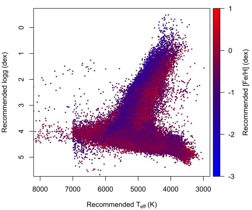
E. Pancino et al.: The Gaia view of Johnson-Kron-Cousins standards

they all had very few measurements in the oldest of the source           3.3. Gaia photometric quality flag
catalogues. Apart from these cases, we found that the typical
spreads in the pairwise magnitude differences was about 1–2%             The precision and accuracy of the Gaia EDR3 photometry is un-
(Figure 3), depending on the band. The spreads of the paired dif-        precedented, especially for the relatively bright stars in common
ferences were generally not compatible with the squared sum of           with the Landolt and Stetson collections presented here: stan-
the formal uncertainties on each pair, being on average larger by        dard errors of a few mmag or better and an overall zeropoint
a varying amount. We thus multiplied the original Landolt un-            accuracy of better than 1% (Riello et al. 2021; Pancino et al.
certainties by the ratios reported in Figure 3, i.e., 5.8 for the U      2021). Thanks to the numerous parameters published in the Gaia
band, 1.5 for the B and R bands, 2 for the V band, and 1.4 for the       catalogue, we can perform a variety of quality assessments. In
I band. The re-calibrated uncertainties are reported in Table 1.         the next section we will deal with the risk of contamination and
Stars with repeated entries in different Landolt source catalogues       blends by nearby stars and binary companions. Here, we will use
were flagged (Duplicates column in Table 1).                             those parameters that are most relevant to evaluate the photomet-
                                                                         ric measurement quality. We started by flagging (not removing)
     The resulting catalogue of unique stars contained 683 stars
                                                                         stars with:
with one or more neighbors, i.e., with possible alternate matches,
albeit with a lower figure of merit (as defined by Marrese et al.            – a BP magnitude lower than 20.3 mag, following the recom-
2019). To verify whether any neighbor could be a better match                  mendation by Riello et al. (2021);
than the originally chosen best match, we computed the expected              – a two-parameter solution, i.e., without proper motion and
G magnitude from Landolt V and V–I, using both the relations                   parallax determination (Lindegren et al. 2021b) and, what
by Riello et al. (2021) and the ones presented in Section 5.1, and             is more important here, without BP and RP magnitudes;
we studied the distribution of differences between the original              – a relative error on the flux of the G, GBP , and GRP magnitudes
and expected Gaia magnitudes. On the one hand, we found that                   larger than the 99th percentile as a function of magnitude,
neighbors were generally fainter in Gaia than expected from the                similarly to what done in Sections 2.1 and 2.2 for the ground-
V and I magnitudes in the Landolt collection. On the other hand,               based photometric quality;
the best matches had expected G magnitudes compatible with                   – a fraction of BP or RP contaminated transits higher than 7%
the V and I Landolt magnitudes, within uncertanties. We thus                   (following Riello et al. 2021), indicating that the mean pho-
concluded that the best matches – according to the astrometric                 tometry could be significantly disturbed by nearby (bright)
figure of merit – were also best matches according to photome-                 stars, located outside of the BP/RP window assigned to the
try. Therefore, we kept the best match in the catalogue, but we                star itself.
flagged all stars with neighbors (Neighbors column in Table 1).
                                                                             In practice, the Gaia quality flag GaiaQual (Table 5) counts
                                                                         how many of the above quality criteria were not fulfilled, i.e., a
3.2. Stetson cross-match analysis                                        zero flag means that all criteria were passed (best quality), one
For the Stetson collection, the database snapshot downloaded in          that one quality criterium was not met, and so on. In the Landolt
April 2021 contains 204 303 individual entries. In the field of the      collection, 98% of the stars with a Gaia match met all the quality
Carina dwarf galaxy, we found almost 5000 stars with the same            criteria, while no star failed all the criteria. In the Stetson collec-
ID and photometry, and slightly different coordinates. These du-         tion, 82% of the stars with a Gaia match passed all the quality
plicates were removed before performing the cross-match and              criteria, while only one star failed all criteria.
are not included in the figure above. Of the 4970 stars without
a Gaia match, about 4550 are too faint to be observed by Gaia,           3.4. Probable blends and binaries
while the remaining '450 are mostly located in the Hydra I clus-
ter field. Even when trying a wide cone search (20") and then            As a space observatory with a typical PSF (Point Spread Func-
selecting the best neighbors based on magnitudes, we could not           tion) size of 0.177", Gaia can help in flagging potentially dis-
recover unambiguously these stars in the Gaia catalogue.                 turbed sources, either by chance superposition with other stars
    Only one unrecognized duplicate object was found in the              on the plane of the sky (blends) or by gravitationally bound bi-
Stetson collection7 , thus no independent statistical analysis of        nary companions. Among the astrometric quality indicators in
the reported uncertainties was possible. We therefore used the           the Gaia EDR3 main catalogue (Lindegren et al. 2021b; Fabri-
comparison with the Landolt collection to re-calibrate the Stet-         cius et al. 2021), we used the following for the purpose:
son uncertainties, which are reported in Table 2 (see Section 4.2
for details). The stars with at least one neighbor are 19073 and             – IPDFracOddWin is the fraction (in percentage) of Gaia tran-
the number of neighbors is reported in the Neighbors column                    sits8 that had disturbed windows or gates, indicating that
in Table 2. Similarly to the case of the Landolt collection, the               those transits are likely to be contaminated by a possible
neighbors do not only have a lower figure of merit based on their              companion (or a spurious source); we conservatively flagged
positions and motions, but they also tend to have Gaia mag-                    all stars with more than 7% of disturbed transits;
                                                                             – IPDFracMultiPeak is the fraction (in percentage) of the
nitudes systematically fainter than expected from their V and
                                                                               Gaia transits with double or multiple peaks detected in the
I magnitudes, using both the relations by Riello et al. (2021)
                                                                               PSF; we conservatively flagged all stars with more than 7%
and our own relations from Section 5.1. Conversely, the best
                                                                               of multiple-peak transits (Figure 4, see also Mannucci et al.
matches have compatible measured and expected Gaia magni-
tudes, within uncertainties. Therefore, we kept the best matches         8
                                                                            We recall here that different Gaia transits are oriented with different
in all cases.                                                            position angles on the sky, and thus the presence of truncated windows,
                                                                         or the relative along-scan distance the presence of multiple peaks, can
7
   This is PG2336+004(A), with identical coordinates and different       vary significantly from transit to transit. Because the angle coverage
magnitudes. Only the B and V magnitudes are available, with largely      for each source changes on the sky depending on the scanning law, the
discrepant values in the two entries. We adopted the weighted mean and   best threshold can be determined empirically, depending on the specific
error of the two entries.                                                stellar sample in hand. See also Figure 4.

                                                                                                                     Article number, page 5 of 19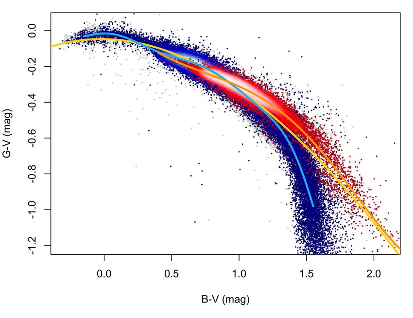
A&A proofs: manuscript no. PhotSets

                                                                             Table 3. Dictionary for the stellar classification labels in the StarType
                                                                             column in Tables 4 and 5. A colon ":" added after the Acronym in the
                                                                             StarType column indicates an uncertain or suspected classification.

                                                                              Acronym              Description
                                                                              BYDRA                BY Draconis type rotational variables
                                                                              CB                   Close Binary
                                                                              CnB                  Contact binary
                                                                              COOL                 Cool Main Sequence star, mostly K or M
                                                                              DCEP                 Classical Cepheid variable (δ Cephei type)
                                                                              DSCT                 Low-amplitude δ Scuti type variables)
                                                                              EA                   Detached Algol-type binary
                                                                              EB                   β Lyrae type binary
                                                                              EW                   W Ursa Majoris type binary
                                                                              GCAS                 γ Cassiopeiae type variable (rapidly rotating
                                                                                                   early type stars with mass outflow)
                                                                              HOT                  Hot star, mostly OBA main sequence
                                                                              HOT_SD               Hot Sub-dwarf
                                                                              L                    Red irregular variable
                                                                              LP                   Long period variable
                                                                              LPSR                 Long period semi-regular variable
                                                                              MIRA                 Mira type variable
                                                                              MS                   Main Sequence Star, mostly AFGK
                                                                              PN                   Central star of a Planetary Nebula
                                                                              R                    Rotational variable
                                                                              RG                   Red giant star
                                                                              RC                   Red clump star
                                                                              RRAB                 RR Lyrae with asymmetric light curves,
                                                                                                   fundamental mode
                                                                              RRC                  RR Lyr with nearly symmetric light curves,
Fig. 4. Example of quality thresholds: each panel shows the logarithmic                            first overtone
histogram of some of the explored Gaia EDR3 parameters, for the Lan-          RRD                  Double Mode RR Lyrae variables
dolt (cyan) and Stetson (orange) collections. The recommended thresh-         ROT                  Spotted stars showing rotational modulation
olds by Lindegren et al. (2021b), Fabricius et al. (2021), and Riello
                                                                              RSCVN                RS Canum Venaticorum rotational variables
et al. (2021) are indicated by grey dotted vertical lines, while our final
adopted ones are indicated by black solid lines.                              SB1                  Single-lined spectroscopic binary
                                                                              SB2                  Double-lined spectroscopic binary
                                                                              SBVC                 Spectroscopic binary or variable candidates
      2022, where this indicator was used to reliably select double           SD                   Sub-dwarf
      QSO candidates with separations of 0.3"-0.6");                          SR                   Semi-regular variable
    – RUWE is the renormalized unit weight error of the astromet-             T2CEP                Type II Cepheid (no sub-classification)
      ric solution; for well behaved stars it should be around one            T2CEP_WVIR           W Virginis type variables (Cepheid)
      and Lindegren et al. (2021b) suggested a cut of  2 σC∗ .              met all criteria, while 39 stars failed them all.

    Similarly to what was done in the previous section, the
GaiaBlend flag (Table 5) indicates the number of the above cri-              3.5. Binary stars
teria that failed. Thus, a flag of zero means that the star passed           To identify spectroscopically confirmed binaries, we used the
9
   In the Stetson collection, some secondary standards are located in        Survey of Surveys (hereafter SoS, Tsantaki et al. 2022), which
globular clusters, but they are generally relatively bright and isolated,    combines in a homogeneous way data from the major spectro-
and of good quality, thus a RUWE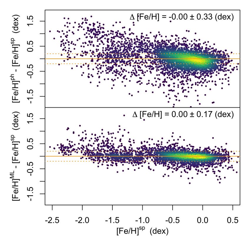
E. Pancino et al.: The Gaia view of Johnson-Kron-Cousins standards

Table 4. Details on notable stars with non-zero VarFlag and/or              – when the variability class was certain in one catalogue and
BinFlag in Table 5. Stars found in more than one external catalogue           uncertain in another (with a colon ":" appended), we chose
have repeated entries in this table.
                                                                              the certain one (i.e., ROT over ROT:);
                                                                            – if all classifications were uncertain, but one specified a class,
      Column             Description                                          we chose the more specific one (i.e., ROT: over VAR:);
      Star ID            Star ID from Table 5                               – if two or more classifications were concordant, we chose the
      Gaia EDR3 ID       Gaia Source ID from EDR3                             most specific one or the one indicating the subcategory (i.e.,
      External ID        ID in the external catalogue                         ROT over VAR, or RSCVN over ROT);
      Source             External catalogue                                 – if classifications were discordant at any level (category or
      StarType           External classification (Table 3)                    sub-category) we indicated them all separated by a slash (i.e.,
                         (":" means suspected or uncertain)                   EW/EB).
      Notes              Any additional notes
                                                                           A dictionary of all the adopted StarType labels can be found
                                                                       in Table 3. In the main combined catalogue (Table 5), we just in-
a star is a spectroscopic confirmed binary in any of the surveys,      dicated whether the star is a variable using the column VarFlag,
using information from Price-Whelan et al. (2020) and Kounkel          that is zero for non-variable stars and one for variable stars; the
et al. (2021) for APOGEE, Traven et al. (2020) for GALAH,              variable type was indicated in the StarType column and the star
Merle et al. (2017) for Gaia-ESO, Birko et al. (2019) for RAVE,        was excluded from the clean sample (Qual=1). In that table, the
Qian et al. (2019) for LAMOST, and Tian et al. (2020) for Gaia         StarMethod column reports the string "Variable – see Table 4".
DR2. Because the SoS is based on Gaia DR2, we used the Gaia            We then provided more details in Table 4, where stars identified
DR2-EDR3 cross-match described at the beginning of Section 3.          as variables in multiple catalogues have multiple entries, and the
In addition, we also searched the CoRoT (Deleuil et al. 2018)          original classification from the corresponding literature source is
and the Kepler (Kirk et al. 2016) catalogues for binary stars.         reported in StarType for each entry.
    As a result, we found 301 unique confirmed binaries (308               We note here that some of the confirmed or suspected vari-
when counting detections in multiple catalogues), of which 35          ables in the Landolt collection are part of some of the most
from the Landolt collection and 266 from the Stetson collec-           widely used selected areas, for example around Mark A, Ru 152,
tion. About half of the 301 stars are classified as close bina-        T Phe, some of the PG standards, and in the SA98, SA104,
ries by APOGEE (Price-Whelan et al. 2020; Kounkel et al.               SA107, SA110, and SA113 standard fields.
2021), the others are SB2, contact binaries, radial velocity vari-
ables, or ultra-wide binaries. We have set a flag for these stars,
                                                                       4. The combined catalogue
BinFlag=1, in Table 5. Their classification, according to the dic-
tionary in Table 3, is stored in the StarType column in Table 5,       We detail in the following sections our procedures to gener-
with an annotation in the StarMethod column stating "Binary            ate the final combined catalogue: we first define a clean sam-
– see Table 4". Of the found binaries, 16 were also classified as      ple (Section 4.1); we then compare the Landolt and Stetson col-
variable stars (next section), thus we included both the binary        lections before merging them (Section 4.2); we further proceed
and the variable classification in the starType column of Ta-          to characterize the stars in terms of reddening, distance, stellar
ble 5, separated by a slash. More details on their classification      type, and astrophysical parameters (Sections 4.3, 4.4, 4.5). A
and literature source can be found in Table 4. The spectroscop-        summary of the catalogue content and format can be found in
ically confirmed binaries, which dominate by number the found          Table 5, which will be available electronically and will also be
binaries, have orbital plane inclinations that tend to be parallel     published at the CDS through the Vizier10 service and at SSDC
to the line of sight. This makes them complementary to the sus-        through the GaiaPortal service11 .
pected astrometric binaries, flagged with GaiaBlend=1 together
with photometric blends, whose orbital planes tend to be perpen-
dicular to the line of sight.                                          4.1. Clean sample
                                                                       Before proceeding, we build a clean sample, that will be used in
3.6. Variable stars                                                    the following analysis and especially in Section 5. Note that all
                                                                       stars will be listed in the combined catalogue, not just the ones
To search for variable stars in the Landolt and Stetson collec-        belonging to the clean sample. We use the criteria:
tions, we examined three different catalogues: (i) the Gaia DR2
catalogue of variable stars (Gaia Collaboration et al. 2019); (ii)          – the photometric quality flags (PhotQual) in the Landolt
the ASAS-SN catalogue of variable stars (Shappee et al. 2014;                 (Section 2.1, Table 1) and Stetson collections (Section 2.2,
Jayasinghe et al. 2018, 2019a,b); and (iii) the The Zwicky Tran-              Table 2) must be smaller than three, meaning that the star
sient Facility (ZTF) catalog of periodic variable stars (Chen et al.          cannot be an outlier in three bands or more;
2020). When appropriate, we used our Gaia DR2-EDR3 cross-                   – the Gaia photometric quality flag GaiaQual must also be
match to identify the stars in the various catalogues.                        smaller than three (Section 3.3);
                                                                            – the Gaia suspected blends and binaries flag GaiaBlend
     We found 117 variables in the Landolt collection and 1416
                                                                              (Section 3.4) must be zero and the star must not be a con-
in the Stetson collection (but see Section 4.4 for additional iden-
                                                                              firmed binary (i.e., BinFlag=0) in any of the scanned binary
tifications of young stellar objects). The majority were unclas-
                                                                              star catalogues (Section 3.5);
sified variables ('900), followed by rotational variables ('250).
                                                                            – the star is not a suspected or confirmed variable (VarFlag
There were 19 variables in common between the Gaia DR2 and
                                                                              and Section 3.6) and in particular is not a suspected or con-
the ASAS-SN catalogue, 37 between ZTF and ASAS-SN, 5 be-
                                                                              firmed YSO (see also Section 4.4);
tween Gaia DR2 and ZTF, and only one star was reported as
variable in all three catalogues. To classify variable stars present   10
                                                                             https://vizier.cds.unistra.fr/
                                                                       11
in more than one catalogue, we adopted the following choices:                http://gaiaportal.ssdc.asi.it/

                                                                                                                   Article number, page 7 of 19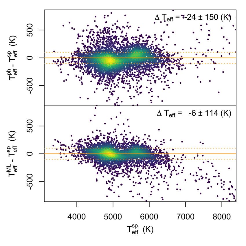
A&A proofs: manuscript no. PhotSets

                                                                          Table 5. Content of the combined secondary standards catalogue.

                                                                           Column          Units     Description
                                                                           Unique ID                 Unique star ID defined here
                                                                           EDR3 ID                   Gaia Source ID from EDR3
                                                                           DR2 ID                    Gaia Source ID from DR2
                                                                           Star Name                 Star Name
                                                                           Collection                Landolt or Stetson
                                                                           RAorig          deg       Original right ascension
                                                                           Decorig         deg       Original declination
                                                                           RAEDR3          deg       Gaia EDR3 right ascension
                                                                           DecEDR3         deg       Gaia EDR3 declination
                                                                           U               mag       U-band calibrated magnitude
                                                                           σU              mag       uncertainty on U
                                                                           nU                        Number of U-band measurements
                                                                           B               mag       B-band calibrated magnitude
                                                                           σB              mag       uncertainty on B
                                                                           nB                        Number of B-band measurements
                                                                           V               mag       V-band calibrated magnitude
                                                                           σV              mag       uncertainty on V
                                                                           nV                        Number of V-band measurements
                                                                           R               mag       R-band calibrated magnitude
                                                                           σR              mag       uncertainty on R
                                                                           nR                        Number of R-band measurements
                                                                           I               mag       I-band calibrated magnitude
                                                                           σI              mag       uncertainty on I
                                                                           nI                        Number of I-band measurements
                                                                           PhotQual                  Photometry quality (Section 2.1, 2.2)
                                                                           GaiaQual                  Gaia quality (Section 3.3)
                                                                           GaiaBlend                 Suspect blend or binary (Section 3.4)
                                                                           BinFlag                   Binary flag (Section 3.5, Table 4)
                                                                           VarFlag                   Variable flag (Section 3.6, Table 4)
                                                                           Qual                      Clean sample has zero (Section 4.1)
                                                                           Dist            (pc)      Distance (Section 4.3)
Fig. 5. The clean Landolt (top panel) and Stetson (bottom panel) sam-
ples, in the absolute and de-reddened V, B–V plane. Stars belonging
                                                                           Distmin         (pc)      Minimum distance (Section 4.3)
to both the Landolt and the Stetson collections are only shown in the      Distmax         (pc)      Maximum distance (Section 4.3)
top panel. The color scales reflect the density of points in the CMD.      E(B–V)          (mag)     Reddening (Section 4.3)
The whole sample of stars with distance and reddening estimates (Sec-      σE(B–V)         (mag)     Reddening error (Section 4.3)
tion 4.3, Table 5) is reported in both panels as grey dots in the back-    StarType                  Classification (Section 4.4, Table 3)
ground. The vertical stripes of stars between the main sequence and the    StarMethod                Classification method (Section 4.4)
white dwarfs, that almost disappear in the clean samples, are mostly       RV              (km/s)    Line-of sight velocity (Section 4.5)
made of relatively faint stars with very uncertain distance estimates.     σRV             (km/s)    RV error (Section 4.5)
                                                                           RVMethod                  Source of the RV
 – as an important exception, the ten reddest stars (V–                    Teff            (K)       Effective temperature (Section 4.5)
   I>3.5 mag) in the Landolt collection with a Gaia match are              σTeff           (K)       Teff error (Section 4.5)
   kept for the following analysis, regardless of their quality            logg            (dex)     Surface gravity (Section 4.5)
   flags, because of the paucity of very red stars in the com-             σlogg           (dex)     logg error (Section 4.5)
   bined collection.                                                       [Fe/H]          (dex)     Iron abundance (Section 4.5)
                                                                           σ[Fe/H]         (dex)     [Fe/H] error (Section 4.5)
    The clean Landolt and Stetson samples are shown in Fig-                ParMethod                 Method for Teff , logg, and [Fe/H]
ure 5. The Landolt clean sample contains 35194 stars (i.e., 76%),                                    (Section 4.5)
while the Stetson one 127467 stars (i.e., 67%), excluding those
in common with the Landolt collection. The final combined cat-
alogue (Table 5) contains a unified Qual flag that is zero for the        less reliably placed on the standard system, and stars close to
clean sample, null for stars without a Gaia match, and one for            the color limits can also be uncertain, because their calibration
the remaining stars.                                                      is based on a handful of standards. In the Landolt collection,
                                                                          the red color limit is extended by about 0.5 mags with respect
4.2. Comparison and catalogue merging                                     to Landolt (1992), while in the Stetson collection by about one
                                                                          magnitude. This has to be taken into consideration when com-
The Landolt and Stetson collections are accurately calibrated on          paring the two collections with each other. For the comparison,
the original Landolt (1992) set of standards, which covers the            we used stars in common between the Landolt and Stetson col-
color range –0.37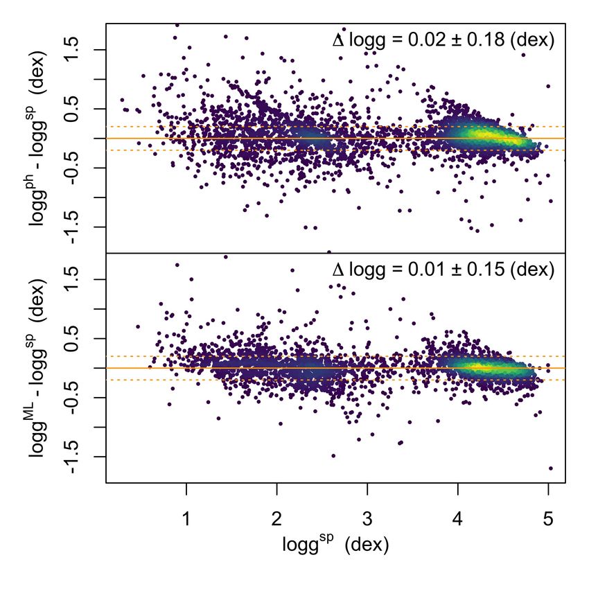
E. Pancino et al.: The Gaia view of Johnson-Kron-Cousins standards

                                                                          cino et al. 2021) and, in addition, the Stetson collection is based
                                                                          on a heterogeneous collection of data from different instruments
                                                                          and filter sets. As anticipated, we can observe a slightly worse
                                                                          agreement (at the 2–3% level) between the Landolt and Stetson
                                                                          collections for stars redder than B–V'2 mag, especially in the
                                                                          R and I bands. The disagreement appears to be systematic, i.e.,
                                                                          it seems to increase with color, and is most probably a conse-
                                                                          quence of the scarcity of red stars in the original Landolt (1992)
                                                                          catalogue, as discussed above. After several experiments, we de-
                                                                          cided not to re-calibrate the R and I magnitudes of the Stetson
                                                                          or Landolt collections, because different calibrations would be
                                                                          required to achieve a better agreement for the M dwarfs and the
                                                                          M giants. However, extra caution should be used when relying
                                                                          on stars redder than B–V'2.0–2.5 mag.
                                                                              For the final, combined catalogue, we chose the Landolt
                                                                          magnitudes when available and the Stetson magnitudes when the
                                                                          Landolt ones were missing12 . All the stars are listed in the com-
                                                                          bined catalogue, including those lacking a Gaia counterpart and
                                                                          those not matching the clean-sample criteria described in Sec-
                                                                          tion 4.1.

                                                                          4.3. Distance and reddening
                                                                          We complemented the combined catalogue with distance and
                                                                          reddening estimates. For Distances, we used the catalogue by
                                                                          Bailer-Jones et al. (2021), based on the Gaia EDR3 parallaxes,
                                                                          who carefully accounted for the relevant parallax biases (Lin-
                                                                          degren et al. 2021b,a). We used their photo-geometric determi-
                                                                          nation, which takes into account the expected color and magni-
                                                                          tude distribution of stars in the Milky Way, to better constrain
                                                                          probable distances. The typical (median) distance is 2883 pc,
                                                                          while only about 25% of the stars are farther than 4883 pc. It
                                                                          is worth noting that the Stetson collection contains more dis-
                                                                          tant stars compared to the Landolt collection, because it targets
Fig. 6. Differences between the Stetson and the Landolt magnitudes        specifically globular clusters and dwarf galaxies with long expo-
for 10769 stars in common, matching the clean-sample criteria (Sec-       sures. We could assign a distance estimate to 96% of the stars
tion 4.1). Each panel reports one of the U BVRI magnitudes as a func-     in the combined collection, but for distant stars the uncertainties
tion of the Landolt B-V, as indicated. The points are colored based on    are of course rather high, with 25% of the stars having distance
the respective Landolt magnitude, and the median differences with their   uncertainties above 40%.
median absolute deviations are reported in each panel. Horizontal lines
and grey-shaded areas mark the zero, ±1, ±3, and ±5% differences. Ver-        For reddening, we explored two different sources: (i) the 3D
tical lines mark the color range covered by the original Landolt (1992)   reddening map by Green et al. (2019), based on Gaia DR2,
catalogue, which defines the Johnson-Kron-Cousins system. The tail of     Pan-STARRS 1 (Chambers et al. 2016; Flewelling 2016), and
faint stars extending upwards in the ∆R panel at about B–V=1.5 mag        2MASS (Skrutskie et al. 2006; Cutri et al. 2012); and (ii) the 3D
is composed by M dwarfs (although other M dwarfs are well behaved)        reddening map by Lallement et al. (2019), based also on Gaia
and could be populated by Hα emitting stars.                              DR2 and 2MASS data. We used the 3D bins in the Green et al.
                                                                          (2019) and Lallement et al. (2019) maps to assign a reddening
                                                                          estimate to each of the stars in the Landolt and Stetson collec-
    Given that we could not renormalize the Stetson collection            tions having a distance estimate in Bailer-Jones et al. (2021).
uncertainties because there was only one duplicated measure-              For more distant stars, or stars with large distance uncertainties,
ment, we can use this comparison instead. If we use the mean              which spanned more than one 3D-bin in the maps, we apdoted
renormalized Landolt uncertainties in each band σLan (Sec-                the weighted average of the E(B–V) estimates corresponding to
tion 3.1) and the spread in the above comparisons σcomp , we can          the best distance estimate, the minimum distance estimate, and
obtain the expected uncertainty in the Stetson collection, σSte           the maximum one. As a result, our E(B–V) estimates often have
considering that σ2comp = σ2Lan + σ2Ste . We thus find that the Stet-     considerably larger uncertainties than the single 3D-bin values
son uncertainties are underestimated by approximately a factor            in the original reddening maps. We studied the differences be-
of two. The re-calibrated uncertainties for the Landolt and Stet-         tween the E(B–V) values derived in this way from the Green
son collections are listed in Tables 1 and 2, and in the combined         et al. (2019) and the Lallement et al. (2019) maps. We found that
catalogue as well (Table 5).                                              – except for about 8% nearby stars with tendentially blue colors
    As expected, the two collections agree to better than 1%              and located in specific areas of the sky – the two sets agree very
with each other in each band, with a spread of 1–3% depend-               well, with a median offset of 0.01±0.05 mag and a mean one of
ing on the band. The U band has the highest spread of about
3%, while the B band displays a spread of 2%, with several dis-           12
                                                                             We also searched for duplicates between the Landolt and Stetson
crepant stars. The bluest bands are notoriously more difficult to         stars without a Gaia EDR3 match. Only a handful were found, and the
standardize (Clem & Landolt 2013; Altavilla et al. 2021; Pan-             Landolt measurements were retained in the combined catalogue.

                                                                                                                 Article number, page 9 of 19
A&A proofs: manuscript no. PhotSets
tion 3.6, confirmed or suspected, were flagged as variables
in the VarFlag of Table 5 and excluded from the clean sam-
ple (Section 4.1);
– 168 white dwarfs from the catalogues by Kong & Luo
(2021), who used LAMOST spectra and literature sources to
confirm their candidates, and Fusillo et al. (2021), who used
APOGEE spectra; we used both the main and the reduced
proper motion catalogues by Fusillo et al. (2021), applying
the recommended probability cuts of 0.75% and 0.85%, re-
spectively; 39 sources were in both the Kong & Luo (2021)
and Fusillo et al. (2021) catalogues;
– we also searched for stars with reliable X-ray counterparts
in the optically cross-matched XMMslew and ROSAT cata-
logues by Salvato et al. (2018) and in the eRosita catalogues
by Salvato et al. (2021) and Robrade et al. (2021); however,
we only found a handful of objects, all with non-stellar X-ray
properties according to the criteria by Salvato et al. (2018),
that were probable false matches.
As an exception, for binary and variable stars, the appropri-
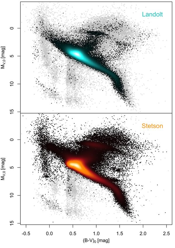
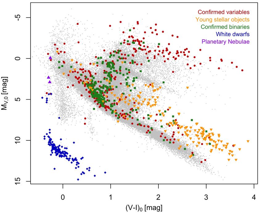
Fig. 7. The position of some stellar types in the absolute and deredde- ate classification from Sections 3.5 or 3.6 was adopted instead of
nend V, V–I plane (see Sections 3.5, 3.6, and 4.4 for more details). The the one based on the CMD. The classification is reported in the
clean sample (Section 4.1) is plotted in grey in the background. StarType column in Table 5, using the acronyms listed in Ta-
ble 3. The classification is accompanied by a StarMethod col-
umn, which details whether the classification was done using the
0.02±0.14 mag. However, the Green et al. (2019) set does not
CMD, the binary or variable analysis, or one of the mentioned
cover the entire sky. We therefore decided to use the Lallement
literature sources.
et al. (2019) maps for sake of homogeneity13 . We could assign
an E(B–V) estimate to 96% of the stars in the combined cata-
logue, i.e., virtually all the stars with a distance estimate. It is 4.5. Stellar parameters
however very important to keep in mind that a large fraction of
the stars in the combined catalogue are farther than the volume Here we characterize the secondary standards in terms of the fol-
covered by the 3D maps and therefore their E(B–V) might be lowing parameters: line-of-sight or radial velocity, hereafter RV;
underestimated. effective temperature, Teff ; surface gravity logg; and iron metal-
licity, [Fe/H]. The goal of this exercise is not to provide the most
accurate parameters. Rather, we found that even a relatively good
4.4. Color-magnitude diagram and stellar classification characterization of stars in the combined catalogue is sufficient
to provide more reliable color transformations between photo-
To characterize the stellar content of the combined catalogue,
metric systems, and in particular it helps in defining the domain
we built the absolute and de-reddened color-magnitude diagram
of applicability of those transformations (see Section 5 for more
(CMD, see Figure 7), using the distance and the E(B–V) deter-
details). We used three different methods to derive stellar param-
mined in Section 4.3. We assumed RV = 3.1 and used Dean et al.
eters: spectroscopy (Section 4.5.1); photometry (Section 4.5.2);
(1978) and Cardelli et al. (1989) to obtain Aλ /AV from E(B–V).
and machine learning (hereafter ML, Section 4.5.3). We then
As a first step, we performed a rough manual classification of
built a recommended set of parameters by choosing the spec-
stars in different categories (main sequence, giants, red clump
troscopic ones when available, then the ML ones, and for stars
giants, hot, cool, subdwarfs, white dwarfs, and so on) based on
lacking both, we used the photometric parameters. To keep track
their position in the above CMD, as indicated in the StarType
of the method used to get parameters for each star, we added
column in Table 5, using the labels in Table 3. Only stars having
the information in Table 5, in the parMethod column. In this
V and I magnitudes, as well as distance and reddening estimates,
way, we could assign some estimate of the stellar parameters to
could be initially classified this way. In the same StarType col-
190651 stars, i.e., 80% of the total. The final set of recommended
umn, we also marked the following specific stellar types from
parameters is displayed in Figure 8, while the comparison among
literature catalogues:
the results of the three methods is shown in Figure 9.
– five central stars of confirmed planetary nebulae, identified
with the catalogue by González-Santamaría et al. (2021); all 4.5.1. Spectroscopic parameters and radial velocity
five are high confidence planetary mebulae according to the
authors (Group A), but only three have good U BVRI pho- The first method we employed is based on spectroscopy. We
tometry in the combined catalogue; used data from the SoS I (Tsantaki et al. 2022, see also Sec-
– 189 young stellar objects (YSO) from the Marton et al. tion 3.5), which contains homogenized, combined, and recali-
(2019) catalogue; these were identified adopting slightly brated RVs for about 11 million stars, with zero-point errors of a
more stringent criteria that the ones recommended by the few hundred m/s and internal uncertainties in the range 0.5–1.5
authors14 ; all YSO from Marton et al. (2019) or from Sec-
tainty δLY is the probability that the object is indeed a young stellar ob-
13
We note that all the stars with an estimate from the Green et al. (2019) ject in all the WISE bands, and SY with its uncertainty δSY is the same
map also had an estimate from Lallement et al. (2019). probability, but without considering the W3 and W4 bands. We classi-
14
We used R>0.5 and LY-δLY≥0.9, or R≤0.5 and SY-δSY≥0.9, where fied as "YSO:", i.e., as suspect YSO, 122 additional objects matching
R is the probability that the WISE detections are real, LY with its uncer- the less-restrictive criteria recommended by the authors.
Article number, page 10 of 19E. Pancino et al.: The Gaia view of Johnson-Kron-Cousins standards
– for stars hotter than 7000 K and 13000 K, we used the two
relations by Deng et al. (2020), which however require (B–
V)0 rather than (V–I)0 ;
– for white dwarfs, we fitted with a third-order polynomial the
(B–V)0 of the WDs having spectroscopic parameters from
Kong & Luo (2021) or Fusillo et al. (2021) and we estimated
a typical 15% uncertainty from the residuals of the fit; we
then applied the relation to all stars classified as WDs ei-
ther spectroscopically or from the CMD (i.e., with StarType
WD or WD:, Section 4.4).
We further assigned Teff to 4244 stars, using the Anders et al.
(2022) catalogue, described in more details below. As can be
seen from Figure 9, a good overall agreement is obtained be-
tween the spectroscopic and photometric temperatures, with a
median difference of ∆Teff =–24±150 K, in the sense that the
photometric temperatures are slightly smaller than the spectro-
scopic ones. For consistency, we corrected the photometric Teff
for this small offset. However, above '7000 K, there are vari-
Fig. 8. The final set of recommended parameters for the clean sample.
ous large trends and substructures – mostly related to WDs and
Only stars having also an [Fe/H] estimate are shown. A long tail of hot hot subdwarfs – and the uncertainties can be substantially higher
stars and the WD sequence are not shown. See Section 4.5 for details. than for cooler stars. We thus obtained photometric Teff for 93%
of the stars in the combined catalogue, i.e., the vast majority of
the stars with distance and reddening estimates (Section 4.3), al-
km/s, depending on each star’s survey provenance. It is based on beit with high uncertainties above '7000 K.
data from Gaia DR2 (Gaia Collaboration et al. 2018); APOGEE To obtain logg estimates, we computed bolometric correc-
DR16 (Ahumada et al. 2020)15 ; RAVE DR6 (Steinmetz et al. tions using the relations by Alonso et al. (1999), Flower (1996),
2020)16 ; GALAH DR2 (Buder et al. 2018)17 ; LAMOST DR5 and Mann et al. (2015), depending on the type of star and the va-
(Zhao et al. 2012)18 ; and Gaia-ESO DR3 (Gilmore et al. 2012)19 . lidity range of the relations. With the bolometric luminosity, we
We found RV estimates for 9643 stars and stellar parameters estimated the radius from fundamental relations, and then logg
for 6365 stars in the combined catalogue. Because only RVs are using the empirical logR∼f(logg) relation by Moya et al. (2018),
carefully re-calibrated in SoS I, to obtain the other stellar param- which is based on a sample of stars hotter than about 5000 K.
eters for stars observed in more than one survey, we simply took For cooler stars, both dwarfs and giants, the logg estimate is
the mean of the parameters presented in Table 8 by Tsantaki et al. much more uncertain than for warmer stars. The photometric
(2022), which is adequate for our present purpose. We comple- logg obtained in this way have a median difference of ∆logg=–
mented the SoS spectroscopic parameters using the white dwarfs 0.2±0.4 dex with the spectroscopic logg, and they show a lot
identified in the Kong & Luo (2021) or Fusillo et al. (2021) cat- of substructure, especially below 5000 K. However, we found
alogues (see also Section 4.4). This way, we could find addi- that the logg estimates obtained by means of machine learning
tional RV estimates for 35 WDs and stellar parameters for 161 by Anders et al. (2022) from photometry and astrometry (see
WDs, that were specifically derived with the use of WD syn- below for more details) are in better agreement with the spectro-
thetic spectra by the authors, comparing them with LAMOST scopic parameters and show a much smoother behavior across
and APOGEE spectra, respectively. For the stars in common be- the CMD, especially for K and M main sequence stars. We thus
tween the two studies, we simply took the average of their val- used the Anders et al. (2022) logg estimates whenever available,
ues, that compared well with each other. and the above photometric ones for 21381 hot stars for which the
Anders et al. (2022) estimates are not available. The comparison
of the logg estimates obtained by combining the two approaches
4.5.2. Photometric parameters yields ∆logg=+0.02±0.18 dex, and we thus obtained photomet-
As a second method, we used the accurate Landolt and Stetson ric logg estimates for 91% of the stars in the combined catalogue.
photometry, together with our preliminary CMD classification, Finally, it is not possible to derive reliable estimates of
to compute photometric Teff and logg estimates. For the Teff [Fe/H] from simple relations based on Johnson-Kron-Cousins
computation we used: photometry. Thus, we used three different literature catalogues,
in the following order or preference:
– for the FGK dwarfs and giants, we used (V-I)0 which is the
least sensitive to metallicity, and the relations by González – The Xu et al. (2022) catalogue, which is based on LAMOST
Hernández & Bonifacio (2009) for dwarfs and giants; DR7 and Gaia EDR3 data, to provide photometric [Fe/H]
– for stars resulting in Teff < 4000 K, we still used (V-I)0 , but estimates based on the stellar loci of stars with known metal-
we relied on the relation by Mann et al. (2015), which are licity; their [Fe/H] estimates show good agreement with the
computed specifically for cool stars; spectroscopic [Fe/H], with no significant trend and just a
small bias: ∆[Fe/H]=–0.07±0.35 dex; these were available
15
https://www.sdss.org/dr16/ for 24240 stars in our combined catalogue;
16
https://www.rave-survey.org/ – The Anders et al. (2022) catalogue mentioned above, which
17
https://www.galah-survey.org/ results from the application of the machine-learning code
18
http://www.lamost.org/public/ StarHorse (Santiago et al. 2016; Queiroz et al. 2018) to
19
https://www.gaia-eso.eu/ the astrometry and the photometry from Gaia EDR3, and
Article number, page 11 of 19A&A proofs: manuscript no. PhotSets
Fig. 9. Comparison between parameters obtained with different methods. The top panels show the differences between the photometric and
spectroscopic parameters, the bottom ones between the machine-learning and the spectroscopic ones. The left panels show the case of Teff , the
middle ones of logg, and the right ones of [Fe/H]. The median difference and MAD are written in each panel. The horizontal lines mark the zero
(perfect agreement), ±100 K (for Teff ), and ±0.2 dex differences (for logg and [Fe/H]), respectively. See Section 4.5 for more details.
to the combined photometry from 2MASS (Skrutskie et al. cited work by Miller 2015; Santiago et al. 2016; Queiroz et al.
2006; Cutri et al. 2012)20 , Pan-STARSS1 (Chambers et al. 2018; Xu et al. 2022; Anders et al. 2022, and references therein).
2016; Flewelling 2016)21 , Skymapper, and AllWISE (Cutri
et al. 2013)22 , matched using the same cross-matched algo- There is a large number of ML techniques in the literature
rithm used here (Marrese et al. 2017, 2019); these data show that can apply to the case presented in this study. The problem
a clear trend when compared to the spectroscopic [Fe/H] at hand, in the ML lexicon, can be categorized as a supervised
(Section 4.5.1) where the metal-poor end at about [Fe/H]'– regression problem. Supervised ML methods are trained on a
2.0 dex is overestimated by about 0.5–1.0 dex, with a large relatively small sample of objects, where the expected output is
scatter, while the metal-rich one at about [Fe/H]'0.5 dex is known (in our case, the spectroscopic Teff , logg or [Fe/H] from
underestimated by about 0.5 dex; we obtained photometric Section 4.5.1). Over this training sample, the algorithm learns
[Fe/H] estimates for 126706 stars, albeit less accurate than how to transform the input variables, which can be an arbitrary
the Xu et al. (2022) ones; number (see Table 6), into the output estimates by minimizing
– the [Fe/H] estimates by Miller (2015), based on SDSS 10 the resulting error. The trained algorithm is then tested on an in-
photometry (Ahn et al. 2014)23 , which are available for dependent sample, where the output is still known but is not pro-
15523 stars in our combined catalogue; these estimates show vided to the algorithm, in order to prove that it can indeed work
a very similar trend with the spectroscopic [Fe/H] estimates in a general case. The size of the sample used for both train-
as the Anders et al. (2022) ones, therefore, we used them for ing and testing is crucial to maximize the performances of the
the 409 stars that did not have an estimate by Anders et al. method. We tested several ML methods, namely: Random Forest
(2022) or Xu et al. (2022); (RF Liaw & Wiener 2002), Probabilistic Random Forest (PRF
– the [Fe/H] estimates by Chiti et al. (2021), based on SkyMap- Reis et al. 2019), K-Neighbours (KN Goldberger et al. 2005),
per photometry (Wolf et al. 2018), which are available for Support Vector Regression (SVR Drucker et al. 1997), Multi-
998 stars in our combined catalogue; these saturate at about Layer-Perceptron (MLP Murtagh 1991). In the end we identified
[Fe/H]'–1.0 dex but are linearly correlated with the spectro- the SVR method to have the best results, outperforming the other
scopic estimates below [Fe/H]'–1.2 dex; we used them for methods by a considerable margin.
12 additional stars without an estimate by other sources.
We initially identified a set of input values for the ML algo-
The comparison between photometric and spectroscopic pa- rithms from the photometric variables present in the catalogue.
rameters is shown in the top panels of Figure 9. ML methods cannot correctly treat empty (null or NaN) values,
thus the major limiting factor on the size of the sample for train-
ing and testing (and on the final number of parametrized stars)
4.5.3. Machine learning parameters is that some parameters, mostly R and U magnitudes, are fre-
quently missing. By minimizing the error, i.e., the difference
Having a sizeable set of stars with reliable spectroscopic param-
between the training parameters and the output ones in the test
eters from the SoS, and keeping in mind the difficulties of ob-
phase, we identified an optimal set of input variables, depending
taining logg and [Fe/H] estimates for field stars from photometry
on the specific parameter that we are trying to estimate and that
(see Figure 9, top panels), we experimented with ML algorithms
are indicated in Table 6. The estimates produced with these input
as well. It has indeed already been shown that purely numerical
parameters sets are labelled with starMethod=ml_gold in the
methods, such as ML techniques, can be successfully employed
catalogue (55231 stars). We also identified two reduced sets of
to estimate stellar parameters from photometric inputs (see the
input variables, which allow the method to be applied to addi-
20
https://www.ipac.caltech.edu/project/2mass tional sets of stars, although with reduced accuracy. These sam-
21
https://panstarrs.stsci.edu/ ples are labelled as (starMethod=ml_silver and ml_bronze)
22
https://wise2.ipac.caltech.edu/docs/release/allwise/ in the combined catalogue, amounting to 102959 and 1075 stars,
23
https://www.sdss3.org/dr10/ respectively. In the case of silver parameters we essentially drop
Article number, page 12 of 19You can also read