The structure of solar radio noise storms - arXiv
←
→
Page content transcription
If your browser does not render page correctly, please read the page content below
Astronomy & Astrophysics manuscript no. ms16˙2˙col                                                                                 c ESO 2018
                                               February 4, 2018

                                                                          The structure of solar radio noise storms
                                                                          C. Mercier1,⋆ , P. Subramanian2 ,⋆⋆ , G. Chambe1,⋆⋆⋆ , and P. Janardhan3 ,†

                                                    1
                                                        LESIA-Observatoire de Paris, CNRS, UPMC, Univ. Paris-Diderot
                                                    2
                                                        Indian Institute of Science Education and Research, Sal Trinity Building, Pashan, Pune -411021, India
                                                    3
                                                        Astronomy and Astrophysics Division, Physical Research Laboratory Ahmedabad - 380 009 e-mail: claude.mercier@obspm.fr
                                                        e-mail: p.subramanian@iiserpune.ac.in
                                                        e-mail: gilbert.chambe@obspm.fr
                                                        e-mail: jerry@prl.res.in
arXiv:1412.8189v2 [astro-ph.SR] 30 Dec 2014

                                                    Received xxx, 2012; Accepted xxx, 2022

                                                                                                                 ABSTRACT

                                                    Context. The Nançay Radioheliograph (NRH) routinely produces snapshot images of the full sun (field of view ∼ 3R⊙ ) at 6 or 10
                                                    frequencies between 150 and 450 MHz, with typical resolution 3 arcmin and time cadence 0.2 s. Combining visibilities from the NRH
                                                    and from the Giant Meterwave Radio Telescope (GMRT) allows us to produce images of the sun at 236 or 327 MHz, with the same
                                                    field as the NRH, a resolution as low as 20 arcsec, and a time cadence 2 s.
                                                    Aims. We seek to investigate the structure of noise storms (the most common non-thermal solar radio emission) which is yet poorly
                                                    known. We focus on the relation of position and altitude of noise storms with the observing frequency and on the lower limit of their
                                                    sizes.
                                                    Methods. We use an improved version of a previously used method for combining NRH and GMRT visibilities to get high-resolution
                                                    composite images and to investigate the fine structure of noise storms. We also use the NRH data over several consecutive days around
                                                    the common observation days to derive the altitude of storms at different frequencies.
                                                    Results. We present results for noise storms on four days. The results consist of an extended halo and of one or several compact cores
                                                    with relative intensity changing over a few seconds. We found that core sizes can be almost stable over one hour, with a minimum in
                                                    the range 31-35 arcsec (less than previously reported) and can be stable over one hour. The heliocentric distances of noise storms are
                                                    ∼ 1.20 and 1.35 R⊙ at 432 and 150 MHz, respectively. Regions where storms originate are thus much denser than the ambient corona
                                                    and their vertical extent is found to be less than expected from hydrostatic equilibrium.
                                                    Conclusions. The smallest observed sizes impose upper limits on broadening effects due to scattering on density inhomogeneities in
                                                    the low and medium corona and constrain the level of density turbulence in the solar corona. It is possible that scatter broadening has
                                                    been overestimated in the past, and that the observed sizes cannot only be attributed to scattering. The vertical structure of the noise
                                                    storms is difficult to reconcile with the classical columnar model.
                                                    Key words. Sun : radio radiation, corona

                                              1. Introduction                                                            field (eg. Mercier et al, 1984, Kai et al, 1985). The apparent size
                                                                                                                         of noise storms is ≤ 3 arcmin. The apparent brightness tempera-
                                              Type I noise storms are the most common non-thermal solar                  ture T b of the continuum can exceed 108 K (Kai et al, 1985) and
                                              radio emission in the decimetric-metric range. Noise storms                even can reach ∼ 1010 K (Kerdraon and Mercier, 1983).
                                              also exist in the decametric range (below 100 MHz) and ex-
                                              hibit different characteristics. These storms are usually referred             The consensus is that radio emission occurs at the funda-
                                              to as decameter noise storms and are not dealt with here.                  mental plasma frequency and is due to suprathermal electrons
                                              Type I noise storms (merely referred to as noise storms from               trapped in closed flux tubes. This explains the strong polar-
                                              now on) can last for hours to days and reveal long-lived pro-              ization in the o-mode and the high values for T b . Theories
                                              duction of suprathermal electrons not directly related to flares           have been proposed by Melrose (1980), Benz and Wentzel
                                              (Le Squeren, 1963). Extensive descriptions have been given by              (1981) and Spicer et al (1982), involving the coalescence of
                                              Elgarøy (1977) and Kai et al (1985). They consist of a broadband           plasma waves with low-frequency waves (ion-acoustic or lower-
                                              continuum (∆ f / f ∼ 1) with superimposed Type I bursts, more              hybrid). Melrose did not specify the origin of fast electrons but
                                              frequent below 250 MHz. Bursts have durations ≤ 0.5 sec and                Benz and Wentzel and Spicer ascribed their production to re-
                                              bandpass ∆ f / f ∼ 3%. They occur in chains of some tens of sec-           connection or to weak shocks associated with newly emerg-
                                              onds with typical intervals 1-2 sec., drifting slowly toward low           ing flux. Subramanian & Becker (2004, 2011) considered a
                                              frequencies. Continuum and bursts are often highly circularly              generic second-order Fermi acceleration mechanism for gener-
                                              polarized in the o-mode of the underlying photospheric magnetic            ating these electrons. They found an overall efficiency ∼ 10−6 for
                                                                                                                         the emission process.
                                               ⋆
                                                                                                                             Only few instruments have produced one-dimensional (1D)
                                              ⋆⋆
                                                                                                                         or two-dimensional (2D) images of noise storms : the Culgoora
                                              ⋆⋆⋆
                                                                                                                         radioheliograph (CRH, 2D, first at 80 MHz, later also at 160,
                                                †
                                                                                                                         320, and 43 MHz, Labrum, 1985), the Nançay radiohelio-

                                                                                                                                                                                               1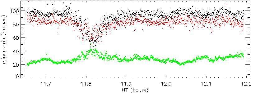
C. Mercier et al.: The structure of solar radio noise storms

graph (NRH), first 1D at 169 MHz, later 2D at 5, 6, or                  were limited to about 6000 λ. Sizes of ∼ 50 arcsec were reported,
10 frequencies from 150 to 450 MHz, Kerdraon & Delouis,                 in general agreement with the results of Zlobec et al, (1992).
1997), the Very Large Array (VLA, 2D at 333 MHz, see eg.                     Some of these results, namely the increase of the observed
http : //www.vla.nrao.edu) and the Giant Meterwave Radio                sizes with decreasing frequencies, are consistent with the classi-
Telescope (GMRT, Ananthakrishnan & Rao, 2002) combined                  cal columnar model (Kai et al, 1985) in which emission at dif-
with the NRH at 327 MHz. The CRH (closed in 1986) and the               ferent frequencies originates at different altitudes in the same
NRH are dedicated to the sun, and the VLA and the GMRT only             flux tube. However, Lang and Willson (1987) pointed out that
occasionally observe it.                                                the observed complexity in the structure of noise storms may
    In principle, imaging noise storms at different altitudes re-       well rule out this simple model. Malik and Mercier (1996) also
quires : i) a field of view wider than the sun since several storms     pointed out that the close positions observed at different frequen-
often coexist, ii) a resolution better than their typical apparent      cies could be difficult to explain with a flux tube in hydrostatic
size to see a possible fine structure, and iii) simultaneous ob-        equilibrium. In fact, very little is known concerning the vertical
servations at several frequencies over their bandpass. Until now,       extent of noise storms. In the absence of stereoscopic observa-
these conditions were never fulfilled at the same time. This ex-        tions, the only possibility is to derive the altitudes of persistent
plains why the structure of noise storms is still poorly known          storms at several frequencies from their apparent rotation (as-
                                                                        sumed to be rigid) during several consecutive days, but this has
    The CRH, the NRH, and the VLA in its compact C con-                 never been done.
figuration (VLA-C) have wide fields of view, but their resolu-               The highest T b values of the continua and the smallest sizes
tion (∼ 1 arcmin) is hardly less than the storm size. No internal       of the continua and bursts are of interest, : the highest values
structure in storms can be observed. Kai et al (1985) reported          of T b constrain the emission theories and the smallest sizes put
that bursts and continuum have approximately the same location          an upper limit to the broadening resulting from the scattering of
and that the apparent size increases with decreasing frequency.         radio waves by coronal density inhomogeneities (Bastian 1994,
This was confirmed by Malik and Mercier (1996) from NRH                 Subramanian & Cairns 2011). Up to now, the highest reported
observations at 164, 236, 327, and 410 MHz. Based on analy-             T b values are of the order of 1010 K, in agreement with the max-
sis of data covering seven days, they also reported that the ob-        imum predicted from plasma emission models. These values,
served positions were close to each other from 236 to 410 MHz,          however, were obtained with a relatively low resolution (> 1
with small changes roughly parallel at the different frequencies,       arcmin), and could have been underestimated.
and that the positions of the bursts and continua widely overlap,
                                                                             The above reviewed observations show that a spatial resolu-
the bursts being slightly narrower. In some cases apparent sizes
                                                                        tion substantially less than 1 arc min (∼ 20 arcsec or less, cor-
are observed down to the resolution. Kerdraon (1973) uses the
                                                                        responding to baselines up to 10000 λ) is needed to properly in-
NRH at 169 MHz, reported sizes of 1.3 arcmin, and Habbal et
                                                                        vestigate the fine structure of noise storms. Only very few such
al (1989), from observations on two days with the VLA-C at
                                                                        high-resolution observations with the VLA are available since
333 MHz, reported sizes of 57 × 47 arcsec. Storms with both
                                                                        its limited field of view restricted studies to a small number of
LH and RH circular polarizations were occasionally reported,
                                                                        intense bursts. The advantage of combining the NRH and GMRT
essentially from early observations with the CRH and from some
                                                                        data, as first presented by Mercier et al (2006) is to get both high
observations with the VLA. However, from a careful analysis of
                                                                        resolution and a wide field of view, allowing them to use the
these reported cases and from an extensive analysis of NRH data,
                                                                        common observations entirely. In this paper, we present results
Malik and Mercier (1996) concluded that there was no evidence
                                                                        from simultaneous observations with the NRH (150, 164, 236,
of bipolar structure and that most of the reported cases should
                                                                        327, 410 MHz) and GMRT (236 or 327 MHz). These frequen-
be either artifacts or (in some cases only) pairs of separate noise
                                                                        cies cover most of the frequency range of noise storms. We give
storms.
                                                                        results for four noise storms observed on different days, with an
     High-resolution (< 10 arcsec) observations with the VLA at         improved NRH/GMRT intercalibration, allowing a better res-
327 MHz in the extended A-configuration revealed some inter-            olution than in Mercier et al (2006). Two cases are complex,
nal fine structure. Lang and Willson (1987) described one storm         with up to three other simultaneous noise storms, and could not
as consisting of four compact sources each about 40 arcsec in           have been investigated without combining the two instruments.
angular diameter, arranged within an elongated 40 × 200 arcsec          This is illustrated in Fig. 1. We also present an analysis of the
source”. However, the time resolution was only 13 and 30 s and          positions of the storms at all the NRH frequencies over several
the dynamical range in images was limited by the small num-             consecutive days before and after the common observations to
ber (12) of the antennas used. Kerdraon et al (1988) presented          investigate their vertical extent.
images of two bursts occuring at different times during a storm,
with typical sizes of 45 arcsec and positions separated by ∼ 50
arcsec, one being polarized and the other unpolarized. Zlobec et        2. Observations, data selection, and processing
al (1992) attempted to derive the smallest spatial scales involved
in noise storms. From observations on two days at 333 MHz,              We used all available joint GMRT / NRH observations of noise
they did not detect any significant power for baselines > 5000 λ,       storms (table 1). Joint observations are possible over ∼ 08:30-
and gave minimum reliable sizes of ∼ 40 arcsec, the smaller             12:00 UT, but those presented here are limited to ∼ 1hour. The
derived sizes being considered as questionable because of the           storm on Aug. 27, 2007, already presented by Mercier et al
poor uv-coverage (not all antennas were available). Mercier et          (2006), is used again since we improved the data processing.
al (2006) combined complex visibilities from the NRH and the            The NRH uses an integration time τ = 0.125 s, shorter than typ-
GMRT at 327 MHz for one day. The resulting images had poten-            ical burst durations, whereas the GMRT uses a longer τ of 2.1
tially the same resolution as with the VLA but had a larger field       or 17 s. The NRH data were integrated over the time intervals
of view. Three noise storms were present, and Mercier et al gave        used by the GMRT. The final time cadence is thus that of the
results for the most intense storm. Because of the difficult in-        GMRT. The time profiles of bursts are therefore smoothed and
tercalibration between both instruments, the accepted baselines         their maximum intensity might be underestimated.

2
C. Mercier et al.: The structure of solar radio noise storms
gains is around 15 %. An absolute flux calibration is achieved
a-posteriori by comparing with NRH visibilities (section 2.3).
2.2. Phase intercalibration
It should be ensured, before combining visibilities, that the storm
positions derived from both instruments coincide within less
than the expected resolution of a few arcsec. Apparent positions
may differ for two reasons: i) both instruments may have dif-
ferent systematic positional errors (up to ∼ 20 arcsec for the
NRH) and, ii) ionospheric effects are different for each instru-
ment. They can be ∼ 1 arcmin at 236 or 327 MHz. We directly
measured the position differences ∆X and ∆Y along the EW and
Fig. 1. Examples of images with the GMRT alone (left) and with
NS directions. A factor exp(−i2π(u∆X + v∆Y)) was then applied
NRH+GMRT(right) for a complex situation on Apr. 06, 2006
to the GMRT complex visibilities before combining them with
at 10:01:28 UT. The intensity scale (shown at bottom) is lin-
the NRH visibilities.
ear from black (lowest level) to red (highest level). The color of
the background (zero level) results from the value of the deep- The position differences ∆X and ∆Y could in principle be de-
est negative artifact. This color scale makes low-level negative rived from the phase differences between the NRH and GMRT
artifacts more visible than the linear black and white scale. The complex visibilities where the uv-coverages coincide, by fitting
resolution (∼ 20 arcsec) is indicated at bottom left. The circle is the phase differences to a linear function of the spatial frequen-
the optical limb. cies u and v. However, there are generally no exact coincidences
and even ”approximate” coincidences are rare, in spite of the
Table 1 : Noise storms observed with GMRT and NRH. NRH uv-coverage density. Indeed the distance between the NRH
and GMRT points should be much less than the variation scale
date GMRT - ——————- NRH ——————— ∼ 1/L of the complex visibility, where L is the typical mutual
τ - ———————- f ———————- distance between solar radio sources. Moreover these phases are
2002 Aug 27 17 164 236 327* 410 432 affected by noise and interference and the procedure would only
2003 Jul 15 2.1 150 164 236* 327 410 432
2004 Aug 14 2.1 150 164 236 327* 410 432
partially use information from both instruments. It follows that
2006 Apr 06 2.1 150 164 236* 327 410 432 ∆X and ∆Y would be uncertain.
τ integration time (s) for GMRT, f frequency for NRH (MHz). Instead, we preferred to directly measure the positions in im-
The common frequency with GMRT is indicated with *. ages separately obtained from the NRH and the GMRT, which
more completely uses information. For this, we limited the
GMRT resolution to the NRH resolution, accepting only GMRT
baselines up to ∼ 3 km. Direct measurement of the position of
2.1. Calibration of each instrument maximum in both images would be affected by rounding errors
The calibration of the NRH is done with Cygnus A about ev- since images are calculated on grids with a finite step (∼ 20 arc-
ery two weeks and is completed with a self-calibration. Since sec in this case). Instead, we measured the barycenter position of
all possible baselines are not achieved, a classical procedure the brightness distribution where it is larger than a given fraction
based on phase closure cannot be used and a specific method m of its maximum. A value m = 0.8 gave good results, ensur-
was developed. This method relies on the fact that the NRH ing also that the obtained positions are not sensitive to possible
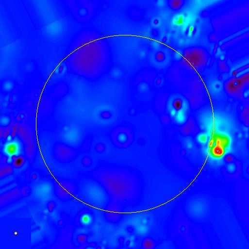
uv-coverage is both dense and regular around the origin. For a extended patterns at low levels. Fig. 2 shows an example: NRH
perfectly phased array, the image of a point source is a sinc- and GMRT north-south positions show partially correlated vari-
like function (at 327 MHz, the beamwidth is ∼ 2 arcmin and ations with time (top), the correlated part being mainly of solar
the field of view is ∼ 1 deg.). With imperfect calibration, side origin. Their difference (bottom) involve mostly timescales ∼ 25
lobes are less regular and larger, especially far from the central minutes, typical of transient ionospheric disturbances. The ac-
beam. Antenna phases are obtained though an iterative reduc- curacy, estimated from the dispersion of points around the solid
tion of the zero and second order momenta of side lobes. Intense line, is < 5arsec. We obtained similar results in the EW and NS
and compact bursts, producing a limited smoothing of side lobes, directions for all days. Given the aspect of the results in Fig. 2,
are used as calibrators. Using baseline redundancies reduces the we adopt a sliding average over two minutes for ∆X and ∆Y.
number of free phases from 48 down to 17, making the proce-
dure more rapid and robust. The accuracy in phase is < 5-10 deg. 2.3. Amplitude intercalibration
and the artifacts on the NRH clean images are reduced to ∼ 5%
and 1-2% for peak and rms values, respectively. The amplitude intercalibration results from comparing ampli-
A typical solar observation sequence with the GMRT com- tudes of the NRH and GMRT complex visibilities in the region
prises around 30 minutes on the Sun, with 30 dB attenuators of good overlap. This occurs for baselines < 1000 m, where the
inserted, followed by around five minutes on a nearby cosmic NRH uv-coverage is dense, excluding baselines < 150 m, which
phase calibrator, with the attenuators removed. This sequence is are lacking in the GMRT. For each data set (i.e., for each snap-
repeated for the duration of the observation. The values of the shot comprising one integration time τ), a multiplying factor C
30 dB attenuators are uncertain by around 10% (0.4 dB). The (applied to the GMRT visibilities) was determined in such a way
automatic gain control mechanism is switched off throughout that the amplitudes of the NRH and GMRT complex visibilities,
the observation. We solve for the antenna gains using data from considered as functions of only the distance to the origin, coin-
the phase calibrator, which are then applied to the solar data. cide at best in the overlapping domain. Ideally, C should remain
The rms uncertainty on the amplitude of antenna + attenuator stable over the common observation duration. This was the case
3C. Mercier et al.: The structure of solar radio noise storms
Fig. 3. Composite images for Stokes I at 327 MHz on Aug. 27,
2002 at 08:27:43. The color scales are linear BW. In the right
frame, the image is saturated at 32% of its maximum. The limits
of the field of view (units of R⊙ ) is (−0.25, +0.80) for EW and
(−0.80, 0.00) for NS. The solid line is the solar limb. The storm
near the western limb is simple. The storms near the center of the
Fig. 2. Top: NS positions (arcsec) versus time (UT) for the main disk are more extended. The aspect of the main storm in Stokes
noise storm on Aug. 27, 2002 for NRH (squares) and GMRT V (not shown) is similar to that in Stokes I. The vertical bars
(asterisks). Bottom: difference between GMRT and NRH NS po- on the left side of images are proportional to log(T B max ), with
sitions (arcsec). The continuous curve gives the sliding average T B max ranging from 106 K at the bottom of the frame, to 1010 K
over two minutes. at its top. Negative artifacts have been suppressed for giving a
dark background at zero level. The relative value of the deepest
negative artifact is proportional to the length of the vertical bars
on the right side, with ticks at 10% and 20%. Same for Fig. 4
for two days (Jul. 15, 2003 and Aug. 14, 2004). For the two other and 5.
days, C was slowly drifting by up to 20%. In order to reduce pos-
sible gain variation effects, we used a sliding average over two
minutes.
2.4. Image calculation
After intercalibration, we obtained snapshot images through the
usual procedure: a Fourier transform of the whole set of data,
followed by a deconvolution. We used the so-called clean proce-
dure, improved with a scale analysis, as described in Mercier
et al (2006). The efficiency of the intercalibrations was then
checked by comparing the results with those obtained by ap-
plying to the GMRT visibilities an extra position shift and/or an
extra amplitude coefficient. Results were globally better without Fig. 4. Composite images for Stokes I. Left: two cores and a halo
such extra corrections. The sensitivity was ∼ 5 arcsec for posi- (all unpolarized) at 236 MHz on July 15, 2003 at 11:16:29. The
tion and 10% for amplitude. Images were better than in Mercier limits of the field of view (units of R⊙ ) are (0.70, 1.15) for EW
et al (2006). The addition of longer baselines resulted in a bet- and (−0.38, +0.07) for NS. Right: three cores and a halo (LH
ter resolution, down to 15 arcsec, taking the final tapering into polarized) at 327 MHz on Aug. 14, 2004, at 11:52:38. The limits
account. of the field of view (units of R⊙ ) are (0.50, 0.96) for EW and
(−0.50, −0.05) for NS. The color scales are linear BW for both
images. The solid lines are the solar limbs.
3. Results
3.1. Qualitative description of the observed storms
For three out of the four observations, there are several noise
storms, one of them being more intense most of the time. For Examples of images are shown in Fig. 3 to 5.
these cases, we focused on the most intense storm. As shown On Aug. 27, 2002 (Fig. 3) there are three storms at 327 MHz.
below, storms can be described as one or several cores with typ- The most intense (T b up to 109 K) is near the western limb, is
ical sizes 30-50 arcsec, embedded in a halo. The polarization compact with a stable position during the observation, whereas
rate can change with position in the storm, but the sense of cir- its intensity fluctuates by a factor up to 8. It consists of only one
cular polarization remains the same. The cores can be followed core. It is strongly polarized, with the same aspect in Stokes I
by continuity. Their positions fluctuate by less than their sizes. and V. The weaker and more extended storms near the center of
Their intensities vary in time by more than a factor 10, appar- the sun have the same sense of polarization as the main.
ently in an uncorrelated way. It can happen that one core be- On Jul. 15, 2003 (Fig. 4 left), there is only one unpolarized
comes much more intense than the other. The storm then ap- storm at 236 MHz, near the western limb. This storm consists
pears simple and compact. In this section, we give a qualitative of an elongated halo with two cores, one being quasi-permanent
description of storm structures from the GMRT / NRH images, at the northern end of the storm, the second (clearly separated)
and a quantitative analysis of their sizes. We derive the altitude appearing only sporadically southward. The positions of cores
of storms at different frequencies using the NRH observations vary (apparently in a random way) by less than their widths. The
over several days. extent of the halo changes with time, extending toward the SE
4C. Mercier et al.: The structure of solar radio noise storms
3.2. Apparent sizes of noise storms
From the descriptions given above, there are two spatial scales
of interest in the structure of noise storms: the overall size, in-
cluding cores and halo, and the size of individual cores.
3.2.1. Overall size of noise storms
The shape of storms can be far from circular and the overall sizes
were derived as follows. At each time, we consider the N points
with brightness between 0.49 and 0.51 T b max , and the smallest
rectangle with sides parallel to the main inertia axes of these
Fig. 5. Composite images for Apr. 06, 2006 at 236 MHz for points and which contains them. The half-power widths along
Stokes I (left) and V (right) at 10:10:27. The color scales are the main axes are defined as the dimensions of the rectangle.
linear BW. The limits of the field of view (units of R⊙ ) are For being robust, the procedure requires N >20. If necessary,
(0.80, 1.25) for EW and (−0.48, −0.03) for NS. The solid line the image was interpolated to fulfill this condition. The accu-
is the solar limb. The brightest core in I is not seen in V. racy on the measured sizes then depends only on the quality of
the image. This quality can be appreciated from the level of the
largest negative artifacts, which can be easily recognized as such
in the cleaned images. These artifacts are always few in number,
their positions are stable and they obviously result from imper-
by up to 4 arcmin. The brightness temperature T b is typically fect calibrations. Their level, larger by more than one order of
2-3 107 K and sometimes reaches 108 K. magnitude than the rms level of the background, is usually be-
On Aug. 14, 2004, three storms are visible at 327 MHz in tween 3% and 15%. They cannot significantly affect the derived
the SW quadrant, separated by several arcmin. The most intense sizes.
storm (S1, shown in Fig. 4 right) is always visible and elongated
from SE to NW. This storm consists of a halo with a banana-
like shape and of several cores, all with LH polarization. Four
cores can be followed, with small changes in position. Three of
them are seen in (Fig. 4 right) : C1 (at NW end) is the most
intense one during most of the time with T b ∼ 3 107 K , but
C2 (at SE end) becomes briefly more intense around 11:48 UT,
with T b = 7.4 107 K. The polarization rates are 60% for C1 and
75% for C2. A fainter storm, southeast of S1, is always present,
with RH polarization. Another faint storm appears sporadically
southwest of S1, with LH polarization.
Fig. 6. Minor axis (arcsec) at 327 MHz of the noise storm on
On Apr. 06, 2006, the situation is still more complex. Up to
Aug. 14, 2004 on composite images versus time (hours, UT) :
four storms are visible at 236 MHz. The most intense storm (S1,
black is for Stokes I, red for Stokes V. The maximum intensity
shown in detail in Fig. 5) lies beyond the western limb, with T b >
is indicated in green (linear scale, arbitrary units).
108 K and sometimes > 109 K, and LH polarization. Weaker
storms can be seen when S1 is not too intense (Fig. 1 right) :
S2, northeast of S1 and near the equator, is also LH polarized, As an example, Fig. 6 shows the variations of the minor
S3 (east of S1) is unpolarized, and S4 (north of S1) is sporadic axis for Aug. 14, 2004: there is a marked minimum, down to
and unpolarized. S1 consists of at least four cores, two or three ∼ 50 arcsec around 11:48 UT, correlated with an increase of
of them often simultaneously visible (exceptionally 4). In Fig. brightness temperature of the core C2. The minor axis is always
5 three cores C1, C2, and C3 (from SW to NE) are visible. In slightly larger in Stokes I than in Stokes V. The dispersion is
Stokes I (left) C1 and C3 are the most intense ones. C2 appears ∼ 5 arcsec. The large axis is about twice as large and has similar
only as a southern extension of C3. In Stokes V (right) only C1 behavior.
and C2 are visible. The position of cores may slightly change On Aug. 27, 2002, the minor axis remains constant at ∼31
with time. Their relative intensity may vary by a factor > 10 on arcsec with very small fluctuations in spite of the intensity vari-
the integration time of the observation (2.1 sec.), apparently in a ations. The major axis slowly increases from 40 to 60 arsec with
random way. The brightness temperature T b may also change by some fluctuations, but the storm is never very elongated. There
a factor ∼ 10 on the same timescale. The sense of polarization are no significant differences between sizes in Stokes I and V.
is the same over the whole storm. The polarization rates range On Jul.15, 2003, the minor and major axes are larger and
from ∼ 80% for C1 down to 1-2 % for C3, and are constant for scattered over 60-110 and 100-160 arcsec, respectively. This
each core. It follows that both shape and size of the storm change large scatter is consistent with the fact that the cores are never
with time, and that they change differently for Stokes I and V : much brighter than the halo. The scatter of both axes decreases
when a core (often C3) strongly dominates (for ∼ 10% of the with time while the intensity of the storm slowly increases.
time), the storm size appears as minimum. On Apr. 06, 2006, both axes shows complex changes,
In summary, for all cases but the first one, the storm structure because of the different time evolutions of the cores. The minor
is complex, with recognizable cores at slightly changing posi- axes are scattered over 35-100 arcsec, and the major axes over
tions, embedded in a more extended halo. The sense of polariza- 70-140 arcsec. Sizes on both axes are minimum for intensity
tion is the same for the cores and the halo, but the polarization peaks. The smallest values of the minor axis (∼ 35 arcsec)
rate may substantially change among the cores. correspond to the intensity peaks of the core C3 (near the limb
5C. Mercier et al.: The structure of solar radio noise storms
and weakly polarized). As for Aug. 27, 2002, these values are Table 2. Extents (rad−1 ) at 50% and 10% levels of the amplitude of the
close to those that are derived below for the cores themselves. complex visibility for cases such as those shown in Fig. 7 , and derived
half-power sizes (arcsec).
Major axes are systematically smaller in Stokes V than in Stokes
I. at 50 % at 10% derived sizes
2002 Aug 27 2700 5900 31
To summarize these results: 2003 Jul 15 1000 2000 87
2004 Aug 14 900 2000 92
– i) The minor and major axes have different behaviors on the 2006 Apr 06 2500 6000 33
four days. The major axis is more variable than the minor
axis because of the presence of several cores, and it is smaller
in Stokes V than in Stokes I because of the lower polarization
degree of some cores.
– ii) There is a anti-correlation between the variations of both
axes and the intensity. The minimum sizes correspond to the
dominance of one core and usually correspond to a large T b .
Conversely, the maximum sizes correspond to several cores
being simultaneously visible. The two storms with the small-
est sizes (Aug., 27, 2002, and Apr. 06, 2006) are also the
most intense.
– iii) In many cases, the overall sizes of storms at half level
Fig. 8. Examples of normalized profiles in Stokes I along minor
do not depend on the halo extent, since the relative level of
and major axes (full and dashed lines) for intense cores on Aug.
the halo is often below 50%. From a visual inspection of the
27, 2002 at 09:01:34 UT (left) and Apr. 06, 2006 at 10:42:28 UT
images, however, the total area where cores appear may be
(right). Abscissas are in arcsec.
large part of the halo. The exception is July 15, 2003, for
which the halo may sometimes extend far toward SE with no
clear presence of cores in this part of the halo. examples of profiles of cores among the narrowest cores along
their main axes for Aug. 27, 2007 and Apr.06, 2006. Similar
3.2.2. Size of cores profiles have also been obtained for Jul. 15, 2003 and Aug. 14,
2004. Table 3 summarizes the results.
Core sizes can, in principle, be deduced from the extent of the Although the overall sizes of storms may substantially
complex visibility V in the uv-plane, at least when the storm is change with time or from one storm to another, the minimum
dominated by an intense core. The amplitude |V| √ then decreases sizes of cores listed in Table 3 are not very different, with the
regularly to small values at distances ruv = u2 + v2 ∼ 1/S possible exception of Jul. 15, 2003, for which the intensity of
from the origin of the uv−plane, S being the size of the core. In the core is never much larger than that of the halo, rendering it
actual cases, |V| decreases less regularly, according to the shape difficult to measure its size.
of the core itself and to the possible contribution of other storms
or cores, but the method can give approximate values of the size Table 3. Smallest minor axes of cores for the four storms.
of intense cores. The extent of |V| is limited to ∼ 2000 λ for
date freq. time ) width
Jul. 15, 2003 and Aug 14, 2004, but it is up to 6000 λ or more
(MHz) (UT) (arcsec)
for Apr. 06, 2006 and Aug. 27, 2002. Fig. 7 shows examples for 2002 Aug. 27 327 09:01:34 31
intense bursts on these two last days. Table 2 summarizes the 2003 Jul. 15 236 11:04:57 57
extent of the |V| at relative levels of 0.5 and 0.1, and the sizes 2004 Aug. 14 327 11:49:04 45
deduced under the hypothesis of Gaussian shapes. These sizes 2006 Apr. 06 236 11:42:28 35
are only indicative and are valid under the above assumptions.
3.3. Heliocentric distances and vertical extents
In the absence of stereoscopic observations, the heliocentric dis-
tances r storm at each frequency can only be derived by following
the apparent position of noise storms during several days and as-
suming a rigid rotation. This can only be done with the daily rou-
tine observations of the NRH at several frequencies. Because of
Fig. 7. Normalized amplitude of Stokes I (solid line) and V the limited NRH resolution, no distinction can be made between
(dashed line) azimuthally integrated complex visibilities versus the positions of bursts and continuum. It is known, however, that
the length of baselines (units of λ) for Aug. 27, 2002, at 09:15:05 these positions may fluctuate from day to day, and even during
UT (left) and for Apr. 06, 2006 at 10:00:19 UT (right). one day (Mercier et al, 1984 at 164 MHz, Malik and Mercier,
(1996 at 164, 236, 327 and 410 MHz). This may introduce er-
rors in the derived altitude, and only the self-consistency of the
The widths of cores can be directly measured from their 1D results gives us confidence in the derived altitudes.
profiles when their intensity sufficiently exceeds that of other The prediction of apparent positions of rigidly rotating
cores and of the halo, after applying approximate corrections for storms needs three parameters (time at the central meridian tran-
the contributions from the halo and from other cores. Fig. 8 gives sit, heliocentric distance, and latitude) and the estimate of the
6C. Mercier et al.: The structure of solar radio noise storms
shift due to refraction. This shift vanishes at the center of the et al, 1988), it can be estimated that H storm values are determined
disk and is maximum at the limb, and it is smaller since emis- within ±10 Mm. In the case of July 15, 2003, the positions at dif-
sion arises in regions denser than the ambient corona. It can be ferent frequencies are so close to each other that it can only be
self-consistently neglected if the predicted positions can satis- said that H storm < 30 Mm.
factorily fit the observed positions during a whole transit on the We introduce for convenience an overdensity factor m as
disk. As an example, Fig. 9 (left) shows the apparent EW posi- the ratio of the density in storms at heliocentric distance r to
tions at 327 MHz of the main storm on April 01-08, 2006 (there that in quiet corona at the same r . The latter is often estimated
was no NRH observation on Apr. 09 and the storm was no longer from the classical Newkirk’s model (1961), which corresponds
visible on Apr. 10). The fit with r storm = 1.27 R⊙ and assuming to an isothermal corona in hydrostatic equilibrium at a temper-
no refraction is satisfactory for the whole period. Fits are better ature T cor = 1.4 MK. It explicitly refers to equatorial regions
at 432 and 327 MHz than at 150 MHz, storm positions being at cycle maximum and is the densest of all models. The com-
more stable at high frequencies. monly cited Saito’s equatorial model (1970) is practically half
The derived r storm are listed in Table 4. From the scatter of as dense. Chambe & Mercier (2012) derived yearly averaged
the data points in plots shown in Fig. 9 (left), the errors can be density models from measurements of the solar radio bright-
estimated as ∼ 0.02 R⊙ . In other words, if refraction effects were ness beyond the limb for the period 2004-2011, both for equato-
included in the model, they would not exceed this value very rial and polar regions, in the same height range as that of noise
much. Note that r storm almost systematically increases with de- storms. Their equatorial models have scale heights similar to that
creasing frequency. of Newkirk’s, but their densities are four times smaller on the av-
erage and decrease by a factor ∼ 2 between 2004 and 2009. For
our practical purpose, we have thus adopted a half dense model
as Newkirk’s, as an average model. The values of m derived for
each observing frequency are displayed in Table 5, in addition
to the scale height H storm and the scale height Hcor of Newkirk’s
model.
The m factor is always substantially larger than unity and
H storm , in spite of its limited accuracy, is significantly less than
Hcor . The implications of these high stom source densities on
the propagation effects, and those resulting from the small scale-
heights H storm on the emission models of storms are discussed in
Fig. 9. Left : apparent EW positions (units of R⊙ ) of the main the following section.
noise storm at 236 MHz from Apr. 1 to 8, 2006. The solid curve
is the fit with r storm = 1.27R⊙ and no refraction. Right : heliocen-
tric distances (units of R⊙ ), versus Ln (frequency) for the same 4. Discussion
storm and linear fit (dashed line). 4.1. Internal structure of noise storms at a single frequency
Kerdraon et al. (1988) observed two bursts at different positions
and times but without relating them to the overall storm struc-
Table 4. Heliocentric distances (units of R⊙ ) of noise storms vs ture. Lang and Willson (1987), from data integrated over one
frequency (MHz). hour, found evidence of fine structure involving several com-
pact sources embedded in a more extended source. They gave
150 164 236 327 410 432
snapshot images (integration time13 and 30 s) from the same
2002 Aug 27 1.25 1.25 1.20 1.18 1.20
2003 Jul 15 1.25 1.24 1.24 1.23 1.23 1.22 observation, showing bursts occurring at different positions, but
2004 Aug 14 1.30 1.27 1.24 1.21 1.18 1.19 they gave no relation between these positions and that of storm
2006 Apr 06 1.33 1.32 1.28 1.27 1.23 1.22 features visible in the time-integrated image.
Our results confirm and extend this description of storms. We
find that they consist of a diffuse region, referred to as the halo,
the extent of which is ∼ 2 arcmin and may change with time,
At all frequencies r storm ≥ 1.2 R⊙ , in agreement with pre- and one or several more compact and brighter cores, embedded
vious studies (Le Squeren 1963, Elgarøy 1977, Mercier and in the halo. The halo does not necessarily exist in all cases and
Kerdraon 1983). The new point is that we have simultaneous its presence cannot be ascribed to instrumental effects. For in-
2D measurements at 5 or 6 frequencies, allowing us to derive stance, combining complex visibilities that are densely sampled
the density scale height in noise storm sources. Assuming that but have a limited extent around the origin (from the NRH), with
the emission
√ frequency f is equal to the local plasma frequency a more extended and sparser set of complex visibilities (from the
f p = 9 n, where n is the electron density (MKS units), and that GMRT) produces an inhomogeneous uv-coverage which could
the scale-height in the storm source H storm = (− 1n dn −1
dr ) , where r result in a composite beam with a core and a halo-like structure.
is the heliocentric distance, is constant for emission between 150 However, the effect of the deconvolution procedure is to correct
and 450 MHz, we can write r = −2 H storm Ln( f ) + K , where the inhomogeneities in the uv-coverage density. Moreover, we
K is a constant. A least square fit of the data shown in Table 4 note that : i) on Aug. 27 (Fig. 3), there is no halo (or very weak)
with this linear relation thus provides H storm . An example of fit around the main storm near the western limb, whereas the source
is shown in Fig. 9 (right) and resulting values of H storm are dis- near the center of the disk is complex with a time-varying halo,
played in Table 5. The typical uncertainty (0.02 R⊙ ) in r storm at ii) on Aug. 14, 2004, the positions of the halo and of the cores
the various frequencies is not much smaller than the differences are stable, but the most intense core is not always the same (often
in height themselves, which results in high relative errors in the at north, then at south at the maximum intensity at 11:48 UT),
derived scale heights H storm . Using a standard procedure (Press and iii) on Jul. 15, 2003, conversely, the extent of the elongated
7C. Mercier et al.: The structure of solar radio noise storms
Table 5. Density scale heights and overdensity m factors in noise storms sources (see text).
Hstorm Hcor - m values at each frequency (MHz) -
Mm Mm 150 164 236 327 410 432
2002 Aug 27 30 (± 10) 108 5.5 12 16 22 28
2003 Jul 15 9 (< 20) 111 4.6 5.2 11 19 30 32
2004 Aug 14 36 (± 10) 111 6.3 6.3 11 17 22 26
2006 Apr 06 35 (± 10) 119 7.5 8.4 14 25 30 32
halo can change within a few seconds, with no changes in the sion concerning the scale height in noise storm sources: the re-
position of cores. These changes cannot arise from instrumental sults of Le Squeren (1963) and Clavelier (1967) seem to indicate
effects and we must conclude that the observed core/halo struc- a large difference in altitudes at 169 and 408 MHz, but their ob-
ture is physical. servations were not simultaneous and were carried out with dif-
Both halos and cores can be visible on most of the snapshot ferent first-generation instruments. Moreover, the high altitudes
images. Although the cores may be recognized from image to found by Le Squeren (1963) are not consistent with those found
image, their position may fluctuate. The changes in their relative by other authors.
intensities seem stochastic and can be large, so that only some of The first multifrequency observations with the NRH at 164,
them can be visible at a given time. At intensity peaks, the image 236, 327, and 410 MHz were reported by Malik and Mercier
is generally dominated by one bright core. Although our obser- (1996). They found that the apparent positions of the continuum
vation rate (2sec) is too slow to distinguish between continuum at different frequencies were often closer to each other than 0.06
and bursts, bursts themselves should originate from cores. The R⊙ and had strongly correlated small-scale motions. However,
sense of circular polarization is the same over the whole extent they did not derive heliocentric distances and consequently gave
of the storm, but the polarization rate may strongly differ from no explicit results on the overdensity of noise storms and on their
one core to another. density scale height.
We obtain, for the first time, heliocentric distances for the
4.2. Apparent sizes of noise storm cores same noise storm at several frequencies, using NRH observa-
tions over several days. These heliocentric distances are in the
At 327 MHz, Lang and Willson (1987) found core sizes of ∼ same range as those found in earlier studies, but the new point
40 arcsec in an image averaged over a period of 1h where the is that they are close to each other at the different frequencies.
storm level was stable (hence presumably for the continuum) This is consistent with the small differences in position with the
as well as in a few snapshot images at times of intensity peaks frequency found by Malik and Mercier (1996). The values of
(presumably for Type I bursts). Zlobec et al (1992) reported sizes the overdensity factor m listed in Table 5 are relative to a model
∼ 50 arcsec for about 20 bursts, with a minimum reliable value similar to that of Saito (1970). Using models from Chambe &
of 40 arcsec for two of them. Kerdraon et al (1988) also reported Mercier (2012) would yield still higher m values.
two bursts with size of 40 arsec. In our study, the main noise These m values would be reduced if storm sources were lo-
storm on Aug. 27, 2002 has a nearly stable size in the 224 images cated in or near active regions (AR). The comparison with im-
during the whole observation of 1 hour, with a minimum of 31 ages from EIT aboard SOHO shows that for all cases but Jul.
arcsec. At 236 MHz, no sizes were previously reported. We find 15, 2003, the noise storms were near the border of active regions
a minimum size of 35 arcsec for some intense bursts from the (AR), yet clearly outside. For Jul. 15, 2003, the storm was be-
core C3 on Apr. 06, 2006. On Jul. 15, 2003, the minimum value tween two AR. Hence for all cases, storms are not located in
of 57 arcsec is less reliable since the corresponding core was high density regions and the m factor should remain large. This
never much brighter than the halo. has consequences for the scattering effect, as discussed below.
In spite of their limited accuracy, the density scale heights
4.3. Coronal density and scale height in noise storm sources in storm sources H storm are found to be smaller than in the am-
bient corona. Two arguments can be given to ensure that this
We recall briefly the results of previous studies on the altitude of result is not biased by refraction. The first involves an estimate
radio noise storms and/or their relative positions at different fre- of the refractive effects needed to account for the apparent po-
quencies. At 408 MHz, Clavelier (1967), using the former EW sition differences between f1 = 432 MHz and f2 = 150 MHz.
1D Nançay interferometer, found a mean r storm ∼ 1.1R⊙ . At 200 If the actual scale height in storm sources was hydrostatic, as in
MHz, Morimoto and Kai (1961), using the 1D Tokyo interfer- the ambient corona, the difference r2 − r1 between heliocentric
ometer, derived the range 1.2-1.3 R⊙ . At 169 MHz, Le Squeren distances of the plasma levels f1 and f2 could be expressed as
(1963), from an extensive study with early versions of Nançay
: r2 − r1 = r1 1−A1 r1 − 1 where r1 and r2 are in units of R⊙
EW and NS interferometers, derived r storm between 1.2 and 1.9
R⊙ , with a mean value 1.5 R⊙ . Using the NRH in its early 2×1D and A = M2kgB0 TR⊙ Ln( ff21 ). Taking T =1.5 MK and r1 = 1.2 gives
version at 169 MHz, Kerdraon and Mercier (1983), obtained the r2 − r1 = 0.48, whereas ∼ 0.1 is observed. A differential shift
mean value 1.22 R⊙ . of 0.38 R⊙ would then be needed to account for the observed
These studies are heterogeneous since most of them used ob- relative positions. Apparent shifts for the positions of sources
servations done with various instrumental limitations (e.g., only at f1 and f2 would be still larger, in contradiction with the fact
one-dimensional resolution, limited position accuracy, single ob- that the maximum refraction effects cannot much exceed ∼ 0.02
serving frequency), and at different stages of the solar cycle. In R⊙ . The second argument comes from Type III bursts, which are
spite of this, a general trend is that noise storms lie relatively produced by fast electron streams accelerated at the borders of
high in the corona, involving larger densities than given by usual AR and propagating along field lines. Their circular polarization
coronal models. It was, however, not possible to draw a conclu- rate is low and it is accepted that the emission takes place at 2 f p .
8C. Mercier et al.: The structure of solar radio noise storms
Their apparent altitude at the limb in the NRH frequency range is which can be partly real. These authors adopt different models
similar to that of noise storms. Thus, if the small position differ- of density fluctuations in the corona, and predict widely different
ences with frequency for noise storm was due to refraction, the broadening of an ideal point source. At 300 MHz, Bastian pre-
same would be expected for Type III bursts. Although no system- dicts apparent sizes of at least several tens of arcsec, well outside
atic study has been done, NRH data usually show larger position the validity domain. In contrast, Subramanian and Cairns, using
differences with frequency than for noise storms. Examples are a lower turbulence level, predict sizes of less than one arcsec.
given by Klein et al (1998). We conclude that the small values Our observations, at the validity limit of the models, show that
for H storm are not due to refraction effects, consistent with the the actual turbulence level, which is presently still poorly known,
fact that these effects must be small because of the high altitude should be intermediate and they could help to specify it.
of noise storms. The constraints on scatter broadening at 327 MHz from our
The fact that H storm < Hcor can be explained in two ways: ei- study are only marginally stronger than from the previous stud-
ther the temperature is very low in the source, ∼ 0.6 MK, which ies, since the minimum size we find (31 arcsec) is not much
seems unlikely for a region where suprathermal particles are pro- smaller than those previously obtained. However, at 236 MHz,
duced through magnetic dissipation, or H storm does not corre- the smallest size we observe (35 arcsec) is hardly larger than
spond to an hydrostatic equilibrium. Since such an equilibrium that at 327 MHz, whereas broadening through scattering is ex-
should be effective along magnetic field lines, this last possibil- pected to scale as 1/ f 2 . In principle, this scaling holds for re-
ity implies that regions emitting at different frequencies do not fractive index µ close to unity but Subramanian and Cairns
lie on the same field line. This leads to the following possible showed that taking into account the departure of µ from unity
sketch for noise storm sources : overdense and compact regions, only brings unimportant changes in the broadening. In any case,
extending normally to the magnetic field with strong density gra- storm sources are compact and overdense and the frequency of
dients normal to the magnetic field. In at least three out of the the emitted radiation is well above the local plasma frequency as
four cases reported here, the density decreases upward. This is soon as it escapes from the source. The fact that we do not find
consistent with our visual experience of NRH data, showing that the expected ratio can be explained in two ways: either the ap-
for most noise storms near the limb, low- frequency sources ap- parent sizes are essentially real, or the turbulence level changes
pear slightly farther from the center of the disk than those at high with time and space. In this last case, the turbulence level should
frequencies. have been more or less the same for the five storms observed
at 327 MHz (including ours) and lower for the two storms we
observed at 236 MHz, particularly for Apr. 06, 2006.
4.4. Implications on the columnar model and the emissions More definite conclusions would require future simultaneous
theories high-resolution imaging at several frequencies (preferably more
than two) of several storms, to separate scattering effects and ac-
Lang and Willson (1987) had already pointed out that the com- tual changes in size with frequency. This is not possible however
plex structure they observed in a noise storm was difficult to rec- with current radiotelescopes. All the storms we reported here
oncile with the simple geometry of the columnar model. We con- were near the limb and that it could be helpful to obtain further
firm this complexity and describe it in more detail. We also add observations such as ours for storms near the center of the disk,
another argument against the columnar model: the density scale where scattering effects are smaller.
height H storm in storm sources, derived from multifrequency ob-
servations, is too small for storm sources at different frequencies
lying along the same magnetic field line, as explained above. 5. Conclusion
This questions the theoretical emission models, which require
trapping of supra-thermal electrons in a closed magnetic loop, We have shown that combining visibilities from the NRH and
from which the columnar model naturally follows. The high po- GMRT works well and is useful, providing snapshot images with
larization rate of storms is usually ascribed to the fact that radio a high dynamical range, a wide field of view, and a high spa-
waves are emitted close to the local plasma frequency, and that, tial resolution. These characteristics were essential in the present
because of the magnetic splitting of the plasma cut-off, only the study since noise storms show internal structure and since sev-
ordinary mode can escape. It is thus difficult to understand how eral storms often coexist. Even with the few cases studied here,
different polarization rates, and particularly very low, can arise we get new insights on the structure of noise storms.
from close sites. It was already known that the electron density in noise storm
sources exceeds that in the ambient corona. We specified over-
As things stand, multifrequency and high-resolution obser- density factors of 5-25 relatively to the widely accepted Saito’s
vations would be useful for better constraining models of noise model, and even more relatively to quiet corona models derived
storms structure and of emission mechanisms. In particular, it is from purely radio observations.
currently not known how the positions of cores at different fre- From multifrequency NRH observations, we derived the
quencies relate to each other. scale height of the electron density in noise storm sources and
showed that it is smaller than in the ambient corona. This im-
4.5. Implication on scattering effects plies that the coronal regions emitting at different frequencies
do not lie along the same magnetic flux tube. This questions the
The apparent size of noise storms is currently explained by classical columnar model and also the current theories for emis-
propagation effects in a turbulent corona. Bastian (1994) and sion mechanism, which imply magnetic trapping of suprather-
Subramanian & Cairns (2011) have modeled these effects mal electrons of a few keV.
assuming small angle scattering for radiation from compact Noise storms appear to have an internal fine structure with
sources embedded in the corona. The limit of validity of this one or several bright and compact cores embedded in a more
assumption has been estimated by Bastian to a broadening of 25 extended halo. The positions of cores fluctuates by less than their
arsec. This is not much smaller than the smallest sizes reported size over a few seconds. Their relative intensities may change
here (31 and 35 arc sec at 327 and 236 MHz, respectively), over time of 2 s, implying that bursts originate from cores. It
9C. Mercier et al.: The structure of solar radio noise storms
follows that the overall apparent shape and size of storms may Malik R., Mercier C., 1996, Ann. Sol. Phys. 165, 347-375.
change rapidly, giving the impression of being quasi-random. Melrose D.B., 1980, Sol. Phys. 67, 357-375.
The sense of circular polarization is the same over the whole Mercier C., Elgarøy Ø., Tlamicha A., & Zlobec P, 1984, Sol. Phys. 92, 375-381.
Mercier C., Subramanian P., Kerdraon A., Pick M., Ananthakrishnan S., &
storm. The polarization rate is stable for each core, but may differ Janardhan P., 2006, A&A, 447, 1189.
between the cores: for Apr. 06, 2006 it is ∼ 80 % for the two Morimoto M., & Kai K., 1961, PASJ 13, 294.
cores at the southern end of the main storm and practically 0 % Newkirk G., ApJ133, 983 - 1013.
for the more intense and elongated core (C3) lying just above Newkirk G., 1967, Annual Review of Astronomy and Astrophysics, Ed.
Goldberg, Ann. Rev. Inc.
(Fig. 5 left). Press W. H., Flannery B. P., Teukolsky S. A., Vetterling W. T., 1998, in
The minimum observed sizes of cores are of interest for dis- Numerical Recipes, 1988, Cambridge University Press, section 14.2, p 504.
cussing scatter broadening. At 327 MHz, we observed a com- Saito K., Ann. Tokyo Astron. Obs. Ser. 2, 12, 53.
pact storm with a remarkably stable size during the whole ob- Saito K., Poland A. I. & Munro R. H., 1977, Sol. Phys., 55, 121.
Spicer D.S., Benz A.O., & Huba J.D., 1982, A&A 105, 221.
servation (1hour), with a minimum value of 31 arcsec, slightly Subramanian, P. & Becker, P. A, 2004, Sol. Phys., 225, 91-103.
smaller than those previously reported (40 arcsec). At 236 MHz, Subramanian, P. & Becker, P. A, 2006, Sol. Phys., 237, 185-200.
the smallest sizes we found (35 arcsec) correspond to the highest Subramanian, P. & Cairns, I., 2011, J. Geophys. Res. 116, A03104,
intensities of a particular core in a complex storm. It is presently doi:10.1029/2010JA015864.
difficult to conclude whether these apparent sizes are real or Zlobec P., Messerotti M., Dulk G.A., & Kucera T., 1992, Sol. Phys. 141, 165-
180.
broadened by scattering, considering that the predictions of cur-
rent theories are limited by the poor present knowledge of the
turbulence level and of its space and time variations. In addition,
there are too few reliable observations with high spatial reso-
lution. More observations of storms at various solar longitudes
could be helpful. However, conclusive observations of storms
at several simultaneous frequencies with high spatial resolution
(< 10 arcsec) and time resolution (< 1sec), in order to observe
the same storm at different levels and to clearly separate bursts
and continuum, does not appear appear feasible with currently
operating instruments.
Acknowledgements. We thank Stephen White who edited the GMRT data of
April 06, 2006 when he was a visiting scientist in Meudon in July 2006. P.
Subramanian acknowledges partial support from the CAWES-II program, ad-
ministrated by the Indian Space Research Organization. We also thank N. G.
Kantharia and S. Ananthakrishnan for helpful discussions regarding GMRT ob-
servation procedures, and an anonymous referee for helping us improve the
manuscript.
References
Alissandrakis C. E., 1994, Adv. Space Res. 14, p(4)81.
Ananthakrishnan S. and Pramesh Rao, A., 2002, Giant Metrewave
Radio Telescope, in Proc. Int’l Conf. on Multicolour Universe,
Eds. R.K.Manchanda and B.Paul, TIFR, Mumbai, 233. Available at
http://www.gmrt.ncra.tifr.res.in/gmrt− hpage/Users/doc/doc.html
Bastian, T. S., 1994, ApJ426, 774-781.
Benz A. O., & Wentzel D.G., 1981, A&A, 94, 100.
Chambe G., Mercier C., 2012, in Understanding Solar Activity : Advances and
Challenges”, M. Faurobert, C. Fang and T. Corbard (eds), EAS Publication
Series, 55, 213.
Clavelier B, 1967, Ann. Astrophys. 30, 895.
Elgaroy O, 1977, Solar Noise Storms, Pergamon press (International Series in
Natural Philosophy).
Habbal S.R., Ellman N.E., & Gonzalez R., 1989, ApJ342, 592-603.
Kai K., Melrose D. B., & Suzuki S., 1985, in S olar Radiophysics, ed. D.J.
McLean and N.R. Labrum, (Cambridge University Press), p 415.
Klein K.-L., 1998, in Second Advances in Solar Physics Euroconference, ASP
Conference Series, C.E. Alissandrakis and B. Schmieder eds., Vol 155, 182.
Klein K.-L., Krucker S., Lointier G., Kerdraon A., 2008, A&A 486, 589-596.
Kerdraon A., 1973, A&A 27, 361.
Kerdraon A., & Delouis J.-M., 1997, in Coronal Physics from Radio and Space
Observations, Proceedings of the CESRA workshop held in Nouan le
Fuzelier, ed. G. Trottet (Berlin Springer), 192.
Kerdraon A., Lang K.R., Trottet G., Willson R.F., 1988, Adv. Space Res. Vol. 8,
No 11, 45.
Kerdraon A., Mercier M., 1983, A&A 127, 132-134.
Kerdraon A., Mercier M., 1983, in Solar Radio Storms, CESRA Workshop 4
held in Duino, 9-13 August, 1982. Edited by A. O. Benz and P. Zlobec.,
p.27.
Labrum N. R., 1985, in Solar Radiophysics (McLean and Labrum eds),
Cambridge University Press.
Lang K.R., Willson R.F., 1987, ApJ, 319, 514.
Le Squeren A.M., 1963, Ann. Astrophys. 26, 97.
10You can also read