Multifractality of light in photonic arrays based on algebraic number theory - Nature
←
→
Page content transcription
If your browser does not render page correctly, please read the page content below
ARTICLE
                  https://doi.org/10.1038/s42005-020-0374-7                  OPEN

                  Multifractality of light in photonic arrays based
                  on algebraic number theory
                  Fabrizio Sgrignuoli1, Sean Gorsky1, Wesley A. Britton2, Ran Zhang2, Francesco Riboli3,4 & Luca Dal Negro1,2,5 ✉
1234567890():,;

                  Many natural patterns and shapes, such as meandering coastlines, clouds, or turbulent flows,
                  exhibit a characteristic complexity that is mathematically described by fractal geometry.
                  Here, we extend the reach of fractal concepts in photonics by experimentally demonstrating
                  multifractality of light in arrays of dielectric nanoparticles that are based on fundamental
                  structures of algebraic number theory. Specifically, we engineered novel deterministic pho-
                  tonic platforms based on the aperiodic distributions of primes and irreducible elements in
                  complex quadratic and quaternions rings. Our findings stimulate fundamental questions on
                  the nature of transport and localization of wave excitations in deterministic media with multi-
                  scale fluctuations beyond what is possible in traditional fractal systems. Moreover, our
                  approach establishes structure–property relationships that can readily be transferred to
                  planar semiconductor electronics and to artificial atomic lattices, enabling the exploration of
                  novel quantum phases and many-body effects.

                  1 Department of Electrical & Computer Engineering and Photonics Center, Boston University, 8 Saint Mary’s St., Boston, MA 02215, USA. 2 Division of

                  Materials Science & Engineering, Boston University, 15 Saint Mary’s St., Brookline, MA 02446, USA. 3 Instituto Nazionale di Ottica, CNR, Via Nello Carrara 1,
                  50019 Sesto Fiorentino, Italy. 4 European Laboratory for Nonlinear Spectroscopy, via Nello Carrara 1, 50019 Sesto Fiorentino, Italy. 5 Department of Physics,
                  Boston University, 590 Commonwealth Ave., Boston, MA 02215, USA. ✉email: dalnegro@bu.edu

                  COMMUNICATIONS PHYSICS | (2020)3:106 | https://doi.org/10.1038/s42005-020-0374-7 | www.nature.com/commsphys                                                1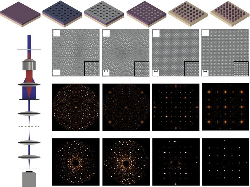
ARTICLE                                                                COMMUNICATIONS PHYSICS | https://doi.org/10.1038/s42005-020-0374-7

I
    n recent years, the engineering of self-similar structures1 in          as two-dimensional cross sections of the irreducible elements of
    photonics and nano-optics technologies2–7 enabled the                   the Hurwitz and Lifschitz quaternions48. These arrays have
    manipulation of light states beyond periodic8 or disordered             recently been shown to support spatially complex resonances with
systems9,10, adding novel functionalities to complex optical                critical behavior49 akin to localized modes near the Anderson
media11–14 with applications to nano-devices and metamater-                 transition in random systems40,44. Figure 1a outlines the process
ials15–17. The concept of multifractality (MF), which describes             flow utilized for the fabrication of the arrays (details can be found
intertwined sets of fractals18–20, was first introduced in order to          in the Methods section). Scanning electron microscope (SEM)
analyze multi-scale energy dissipation in turbulent fluids20 and             images of the fabricated devices are reported in Figs. 1b, e, whereas
broadened our understanding of complex structures that appear in            their geometrical properties, illustrated in Supplementary Figs. 1
various fields of science and engineering21. Specifically, multifractal       and 2, are discussed in the Supplementary Note 1. The multi-
concepts provided a number of significant insights into signal               fractality in the optical response of these novel photonic structures
analysis22, finance23–25, network traffic26–28, photonics12,29–35             is demonstrated experimentally by analyzing the intensity fluc-
and critical phenomena36–42. In fact, critical phenomena in dis-            tuations of their scattering resonances that are measured using
ordered quantum systems have been the subject of intense theo-              dark-field scattering microscopy across the visible spectral range.
retical and experimental research leading to the discovery of               Before addressing the multifractal nature of the measured scat-
multifractality in electronic wave functions at the metal-insulator         tering resonances, in the next section we discuss the far-field
Anderson transition for conductors36,40, superconductors38, as well         diffraction properties of the fabricated arrays because they provide
as atomic matter waves43. The multifractality of classical waves has        insights on the fundamental nature of these novel aperiodic
also been observed in the propagation of surface acoustic waves on          systems.
quasi-periodically corrugated structures35 and in ultrasound waves
through random scattering media close to the Anderson localiza-             Spectral characterization of fabricated arrays. Aperiodic sys-
tion threshold44.                                                           tems can be rigorously classified according to the nature of their
   Considering the fundamental analogy between the behavior of              Fourier spectral properties. In fact, according to the Lebesque
electronic and optical waves10, the question naturally arises on            decomposition theorem50, any positive spectral measure (here
the possibility to experimentally observe and characterize multi-           identified with the far-field diffraction intensity) can be
fractal optical resonances in the visible spectrum using engineered         uniquely expressed in terms of three primary spectral compo-
photonic media. Besides the fundamental interest, multifractal              nents: a pure-point component that exhibits discrete and sharp
optical waves offer a novel mechanism to transport and reso-                (Bragg) peaks51, an absolutely-continuous one characterized by
nantly localize photons at multiple-length scales over extended             a continuous and differentiable function52 and a more complex
surfaces, enhancing light–matter interactions across broad fre-             singular-continuous component where scattering peaks appear
quency spectra. These are important attributes for the develop-             to cluster into a hierarchy of self-similar structures forming
ment of more efficient light sources, optical sensors and nonlinear          a highly-structured spectral background53,54. Systems with
optical components12,45. However, to the best of our knowledge,             singular-continuous spectra do not occur in nature. Moreover,
the direct experimental observation of multifractal optical reso-           their spectral properties, which are often associated to the
nances in engineered scattering media is still missing.                     presence of multifractal phenomena, are difficult to characterize
   In this paper, we demonstrate and systematically characterize            mathematically51. In this section, we introduce and characterize
the multifractal behavior of optical resonances in aperiodic arrays         the spectral properties of our scattering systems by investigating
of nanoparticles with the distinctive aperiodic order that                  their measured far-field diffraction spectra.
is intrinsic to fundamental structures of algebraic number the-                When laser light uniformly illuminates the arrays at normal
ory46–48. The paper is organized as follows. First, we analyze the          incidence, sub-wavelength pillars behave as dipolar scattering
far-field diffraction spectra of these aperiodic photonic systems,           elements and the resulting far-field diffraction pattern is propor-
which have been conjectured to exhibit singular-continuous                  tional to the structure factor defined by:
characteristics49. Second, we perform dark-field microscopy                                                                  2
measurements to directly visualize the scattering resonances of                                            1 XN
                                                                                                                     ikr j
                                                                                                   SðkÞ ¼         e         ;            ð1Þ
the fabricated structures across the visible spectrum where they                                           N  j¼1
exhibit complex spatial distributions with intensity oscillations at
multiple-length scales. Third, we perform frequency–frequency               where k is the in-plane component of the wavevector and rj are the
correlation analysis that subdivides the measured scattering                vector positions of the N nanoparticles in the array. This is
resonances according to their common structural features,                   demonstrated in Fig. 1, where we compare the calculated structure
enabling a classification that greatly reduces the dimensionality of         factors, shown in Figs. 1f–i, with the measured diffraction
the measured datasets. Finally, we demonstrate that the scattering          patterns, shown in Figs. 1j–m. The optical setup used to measure
resonances of the proposed photonic arrays exhibit strong mul-              the diffraction is schematically illustrated in Fig. 1n and further
tifractal behavior across the entire visible range. Our findings             discussed in the Methods section. The experimental diffraction
show the coexistence of resonant states with different localization         patterns match very well with the calculated ones and display
properties and multifractal intensity fluctuations in deterministic          sharp diffraction peaks embedded in a weaker diffuse background,
two-dimensional structures based on algebraic number theory.                particularly noticeable in the case of Gaussian and Eisenstein
We believe that the results presented here provide yet-unexplored           primes. The coexistence of sharp diffraction peaks with a
possibilities to exploit multifractality as a novel engineering             structured (self-similar) background is characteristic of singular-
strategy for optical encoding, sensing, lasing and multispectral            continuous spectra described by singular functions that oscillate at
devices.                                                                    every length scale49,51,53. The strength of the continuous spectral
                                                                            component weakens progressively from Eisenstein and Gaussian
                                                                            primes to Hurwitz and Lifschitz structures, which display a more
Results and discussion                                                      regular geometry. See also Supplementary Fig. 3 and the related
The investigated devices consist of TiO2 nanopillars deposited              discussion in the Supplementary Note 1.
atop a transparent SiO2 substrate and arranged according to the                A remarkable property of structures that support singular-
prime elements of the Eisenstein and Gaussian integers47, as well           continuous components is that their resonant modes are

2                         COMMUNICATIONS PHYSICS | (2020)3:106 | https://doi.org/10.1038/s42005-020-0374-7 | www.nature.com/commsphys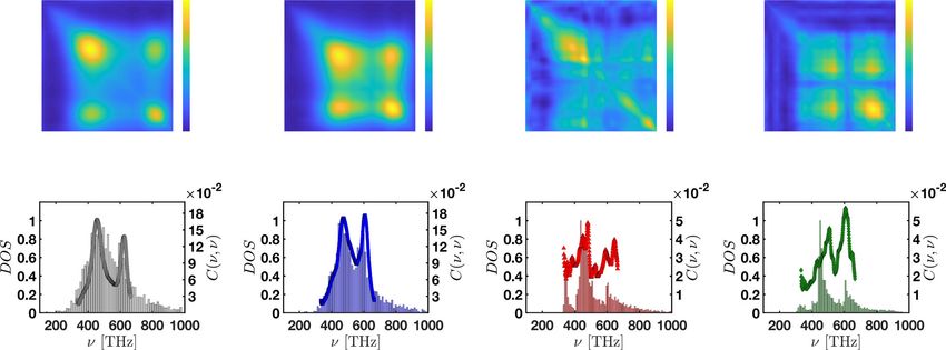
COMMUNICATIONS PHYSICS | https://doi.org/10.1038/s42005-020-0374-7                                                                      ARTICLE

    (a)           SiO2   TiO2      Cr          PMMA

            1 TiO2 deposition            2 EBL             3 Cr Deposition            4 Liftoff               5 RIE              6 Cr Removal

    (n)                                  (b)                       (c)                            (d)                     (e)
       405nm
        laser                   y [µm]
       Sample

      Objective
                                         1µm                       1µm                            1µm                     1µm
                                                  x [µm]                     x [µm]                     x [µm]                     x [µm]
                                         (f)                       (g)                            (h)                      (i)

          IP,AS
                                ky

           FP

                                                      kx                       kx                         kx                            kx
                                         (j)                        (k)                           (l)                     (m)
                                ky

           FP

       Camera

                                                      kx                       kx                         kx                           kx
Fig. 1 Experimental realization of sub-wavelength prime arrays and their diffractive properties. a Process flow used to fabricate the TiO2 nanocylinders
on a SiO2 substrate. b–e Scanning electron microscope images of fabricated samples: b–e Eisenstein, Gaussian, Hurwitz and Lifschitz prime configurations,
respectively. Insets: enlarged view of the central features for each pattern type. Nanocylinders have a 210 nm mean diameter, 250 nm height and average
inter-particle separation of 450 nm. Calculated (f–i) and measured (j–m) k-space intensity profiles corresponding to the prime arrays reported in b–e,
respectively. n Optical setup for measuring far-field diffraction patterns of laser illuminated sample. IP image plane, AS Aperture stop, FP Fourier plane.

critical55–58. Critical modes exhibit local fluctuations and spatial             imaging system in illumination-detection configuration as
oscillations over multiple-length scales that are quantitatively                explained in the Methods section (see also Supplementary
described by multifractal analysis45,59. These peculiar scattering              Note 2). A large dataset of 355 different dark-field scattering
resonances have been demonstrated in one-dimensional aperiodic                  images, for each investigated structure, was collected corre-
systems55–58 and in the propagation of surface acoustic waves on                sponding to the excitation of the scattering resonances at different
quasi-periodically corrugated structures35. In the following, we                frequencies ranging from 333 THz up to 665 THz with a reso-
experimentally demonstrate, using dark-field imaging technique,                  lution of ~0.9 THz.
the multifractal nature of the scattering resonances of aperiodic                  Figure 2 shows representative dark-field images of the scattering
arrays based on generalized prime numbers in the visible range.                 resonances of Eisenstein 2a–d, Gaussian 2e–h, Hurwitz 2i–l and
                                                                                Lifschitz 2m–p arrays collected at different frequencies across the
Dark-field scattering measurements. Dark-field (DF) micro-                        visible range, as specified by the markers in Fig. 3. The scattering
scopy is a well-established technique to image the intensity dis-               resonances of the Eisenstein and Gaussian prime structures display
tributions of the scattering resonances supported by dielectric and             a clear transition from localization in the center of the arrays to a
metallic nanoparticles arrays60,61, to visualize the dynamic of                 more extended nature in the plane of the arrays. On the other
microtubules-associated protein62 and to analyze the formation                  hand, this scenario is far richer for the Hurwitz and Lifschitz
of colorimetric fingerprints of different aperiodic nano-patterned               configurations. In particular, we found that the spatial distributions
surfaces63,64. In this section, we use DF microscopy to directly                of their scattering resonances exhibit the following characteristics:
visualize the distinctive scattering resonances supported by the                (i) weakly localized around the central region of the arrays,
fabricated arrays of nanoparticles at multiple wavelengths across               (ii) localized at the edges of the arrays and (iii) spatially extended
the visible spectrum. In particular, we use a confocal DF micro-                over the whole arrays (more details are provided in Supplementary
scopy setup in combination with a line-scan- hyperspectral                      Note 3, Supplementary Fig. 4 and in the next section).

COMMUNICATIONS PHYSICS | (2020)3:106 | https://doi.org/10.1038/s42005-020-0374-7 | www.nature.com/commsphys                                             3
ARTICLE COMMUNICATIONS PHYSICS | https://doi.org/10.1038/s42005-020-0374-7
(a) 0.7 (b) (c) 1 (d) 1
1.2
0.6 0.8 0.8
1
0.5
0.8 0.6 0.6
0.4
0.6
0.3 0.4 0.4
0.2 0.4
0.1 0.2 0.2 0.2
5µm 5µm 5µm 5µm
(e) 0.7 (f) (g) 1 (h) 1
1.2
0.6 0.8 0.8
1
0.5
0.8 0.6 0.6
0.4
0.6
0.3 0.4 0.4
0.2 0.4
0.1 0.2 0.2 0.2
5µm 5µm 5µm 5µm
1.2 0.8 0.7
(i) 0.7 (j) (k) (l)
0.6 1 0.7 0.6
0.6 0.5
0.5 0.8
0.5
0.4 0.4
0.6 0.4
0.3 0.3
0.4 0.3
0.2 0.2 0.2
0.1 0.2 0.1 0.1
5µm 5µm 5µm 5µm
0.6 1.2 1 1.2
(m) (n) (o) (p)
0.5 1 1
0.8
0.4 0.8 0.8
0.6
0.3 0.6 0.6
0.4
0.2 0.4 0.4
0.1 0.2 0.2 0.2
5µm 5µm 5µm 5µm
Fig. 2 Direct observation of the scattering resonances of prime arrays. Representative multispectral dark-field images of the scattering resonances of
Eisenstein (a–d), Gaussian (e–h), Hurwitz (i–l) and Lifschitz (m–p) prime arrays. These quasi-modes are the scattering resonances that most interact with
their corresponding geometrical supports at a fixed frequency. The scale bars indicate the scattering resonance intensities normalized with respect to the
transmission signal of a reference Ag-mirror and reported in arbitrary units. The x and y axis express the length and the width of the investigated devices
expressed in micron scale.
All the measured scattering resonances exhibit complex spatial defined below65:
distributions characterized by intensity fluctuations at multiple-length
P
n
scales. However, by inspecting Fig. 2, we can also recognize structural 1
n δIðr s ; νÞδIðr s ; ν 0 Þ
features in the intensity distributions that are shared by modes of 0
Cðν; ν Þ ¼ s¼1
n ; ð2Þ
different frequencies (compare for instance Fig. 2j with 2l). In order P
n P 0
to quantitatively classify the measured scattering resonances accord-
1
n Iðr s ; νÞ n Iðr s ; ν Þ
1
s¼1 s¼1
ing to their common structural features, we employ in the next
section frequency–frequency correlation analysis. where the counting variable s identifies the pixel of the intensity I
of the considered dark-field image, n is the total number of pixels,
rs = (xs, yP s) denotes the in-plane coordinates, and δIðr s ; νÞ ¼
Correlation analysis of dark-field scattering resonances. Image Iðr s ; νÞ ½ ns¼1 Iðr s ; νÞ=n describes the fluctuations of the
cross-correlation techniques are widespread in signal processing intensity I (see also the Methods section and Supplementary
where they are used to compare different data and identify Note 3).
structural similarities. In this section, we apply the frequency– The results of the correlation analysis separate the set of
frequency correlation analysis introduced by Riboli et al.65 to a collected scattering resonances into two spectral classes. The first
dataset of 1420 measured scattering resonances. This approach class includes the Eisenstein and Gaussian arrays and is
enables to reduce the enormous complexity of our total dataset characterized by large fluctuations in the correlation matrix
into a few constituent groups of resonances that are identified by concentrated around two distinct spectral regions, as shown in
the frequency–frequency correlation matrix. The off-diagonal Figs. 3a, b. Specifically, these two well-defined spectral regions are
elements of this matrix provide the degree of spatial similarity located at ν ≈ 460 THz and ν ≈ 600 THz, respectively. The off-
between two scattering resonances with frequencies ν and ν′, as diagonal peaks of the correlation matrices reported in Figs. 3a, b
4 COMMUNICATIONS PHYSICS | (2020)3:106 | https://doi.org/10.1038/s42005-020-0374-7 | www.nature.com/commsphysCOMMUNICATIONS PHYSICS | https://doi.org/10.1038/s42005-020-0374-7 ARTICLE
10 -2 10 -2 10 -2 10 -2
350 15 350 350 350
15 4 5
12 12 4
450 450 450 3 450
9 9 3
2
550 6 550 6 550 550 2
1
3 3 1
650 (a) 650 (b) 650
(c) 0 650 (d)
350 450 550 650 350 450 550 650 350 450 550 650 350 450 550 650
(e) (f) (g) (h)
Fig. 3 Frequency–frequency correlation analysis of scattering resonances. a–d Frequency–frequency correlation matrix C(ν, ν′) of Eisenstein, Gaussian,
Hurwitz and Lifschitz arrays, respectively. The white line indicates the diagonal elements, i.e., the normalized variance C(ν, ν) of the scattered intensity.
The different markers identify the frequency location of representative scattering resonances that capture the main features of the correlation analysis.
e–h Normalized variance as compared to the normalized density of states (DOS) as a function of the frequency ν.
show that these resonances are correlated, indicating that their array, as shown in Figs. 2m–p and 3d. This complex scenario is
spatial distributions share common structural features. Moreover, well-reproduced also in our numerical simulations, shown in
a reduction of the intensity fluctuations is observed around ν ≈ Supplementary Figs. 6 and 7. The scattering resonances in the
550 THz in both Eisenstein and Gaussian arrays. All these second class display a more complex spatial structure as
features can also be visually recognized in the spatial distributions compared to the ones of the first class. This is confirmed by
of the selected scattering resonances reported in Figs. 2a–h. In comparing the normalized variance of the frequency–frequency
fact, the representative resonances displayed in Fig. 2, which correlation matrices with the spectral behavior of the computed
correspond to the different markers in Figs. 3a–d, have been optical density of states (DOS) of the systems, which we obtained
identified based on the results of the correlation analysis. using the Green’s matrix spectral method (see the detailed
Specifically, Figs. 2a, c do not share any common features: the derivation in the Supplementary Note 4).
resonance in Fig. 2a shows the maximum of its intensity at the Figures 3e–h present the comparison between the DOS and the
center of the array, whereas the resonance shown in Fig. 2c normalized variance C(ν, ν) (see Methods for more details). The
displays an intensity minimum in the same region. On the other Eisenstein and Gaussian prime arrays feature a DOS with two main
hand, the spatial distributions displayed in Figs. 2b, d are highly peaks demonstrating that their scattering resonances are predomi-
correlated. Similar results are obtained for the Gaussian arrays: nantly located within the two spectral regions identified using the
while the resonances reported in Fig. 2e and in Fig. 2g are not correlation analysis. On the other hand, the behavior of C(ν, ν) and
correlated, the spatial distributions in Figs. 2f, h exhibit a similar of the DOS for the Hurwitz and Lifschitz configurations is far richer
structure. and features multiple spectral regions of strong intensity fluctua-
In the second class, which includes the Hurwitz and Liftschitz tions. Although this comparison remains qualitative in nature, it is
arrays, the C(ν, ν′) matrices are more structured and exhibit consistent with the presence of spectral sub-structures that appear
multi-scale fluctuations spreading over the entire frequency on a finer scales in these arrays, which is typical of aperiodic
spectrum, as shown in Figs. 3c, d. Specifically, their normalized systems with singular-continuous spectra51,53,59. Interestingly, the
variances are characterized by peaks and dips that spread over the classification of our structures into two broad spectral classes may
entire measured spectrum. This characteristic behavior indicates reflect a fundamental number-theoretic difference in the nature of
that the spatial intensity distributions of the measured scattered the corresponding rings. In fact, although the Eisenstein and
radiation rapidly fluctuate with frequency due to the excitation of Gaussian structures are constructed based on the prime elements
pffiffiffiffiffiffiffi of
scattering resonances in the systems. In the Hurwitz configura- the p
rings
ffiffiffiffiffiffiffi associated to the imaginary quadratic fields Qð
pffiffiffi3Þ and
tion, for example, some of these fast fluctuating resonances are Qð 1Þ, which are the commutative rings Z½ð1 þ i 3Þ=2 and
correlated (or anti-correlated), as highlighted by the off-diagonal Z½i, the Hurwitz and Lifschitz structures are constructed based on
elements of the correlation matrix of Fig. 3c. In fact, the scattering two-dimensional cross sections of the irreducible elements of
resonances of the Hurwitz array can be classified in four different quaternions, which form a non-commutative ring66–68.
spectral regions: (i) [350, 420] THZ, (ii) [430, 480] THz, (iii) [480,
600] THz, (iv) larger than 600 THz (see also Supplementary
Fig. 5). Specifically, region (i) is characterized by the same Multifractal analysis of dark-field scattering resonances. In this
scattering resonances of Fig. 2i that are mostly localized at the section, we directly demonstrate that the measured dark-field
center of the array and that are anti-correlated with all the others. scattering resonances of the investigated arrays exhibit strong
On the other hand, modes in region (ii) are correlated with the multifractal behavior. We limit our analysis to the representative
ones in region (iv). This correlation can also be recognized by scattering resonances shown in Fig. 2 that, as previously discussed
visually comparing the scattering resonance of Fig. 2j with the one based on the frequency–frequency correlation matrix, are repre-
reported in Fig. 2l. Finally, region (iii) is populated by scattering sentative of the variety of structural features observed across the
resonances spatially localized at the edge of the arrays, as shown visible spectrum. In order to quantitatively describe intensity
in Fig. 2k. The same considerations apply to the Lifschitz prime oscillations that occur at multiple scales, we apply the multifractal
COMMUNICATIONS PHYSICS | (2020)3:106 | https://doi.org/10.1038/s42005-020-0374-7 | www.nature.com/commsphys 5ARTICLE COMMUNICATIONS PHYSICS | https://doi.org/10.1038/s42005-020-0374-7
2
(a) (b) (c) (d)
1.5
1
0.5
0
1 1.5 2 2.5 1 1.5 2 2.5 1 1.5 2 2.5 1 1.5 2 2.5 3
1.2
1 (e) (f) (g) (h)
0.8
0.6
0.4
0.2
0
-0.5 0 0.5 1 -0.5 0 0.5 1 -1.5 -1 -0.5 0 0.5 -1.5 -1 -0.5 0 0.5 1
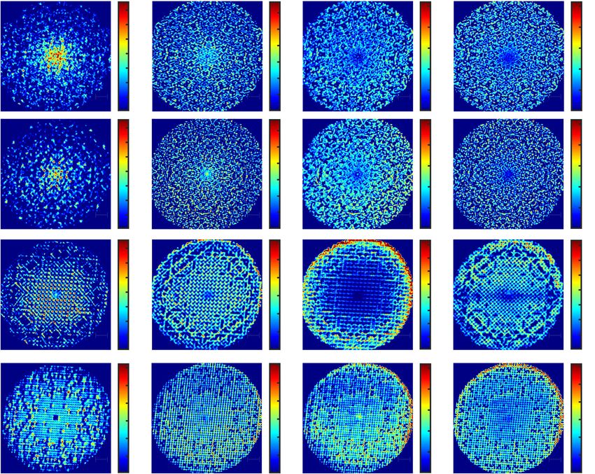
Fig. 4 Multifractal nature of scattering resonances of prime arrays. Multifractal singularity spectra f(α) of the local scaling exponent α (a–d), and
probability density functions Pðln Il Þ of the logarithm of the box-integrated intensity Il (e–h) of representative scattering resonances of Eisenstein (a, e),
Gaussian (b, f), Hurwitz (c, g) and Lifschitz (d, h) prime arrays, respectively. Markers represent the data and the continuous lines in e–h show the best fits
obtained using log-normal function model. Different colors refer to different frequencies corresponding to the main features of their correlation matrices.
Error bars in a–d represent the standard deviations.
scaling method developed by Chhabra et al.19. In particular, we reported in Supplementary Fig. 9 and discussed in the Supple-
employ the box-counting method to characterize the size-scaling mentary Note 6.
of the moments of the light intensity distribution. This is achieved A direct consequence of multifractality is the non-Gaussian
by dividing the system into small boxes of varying size l. We then nature of the probability density function (PDF) of the light
determine the minimum number of boxes N(l) needed to cover intensity distribution near, or at, criticality36,44. We have evaluated
the system for each size l and evaluate the fractal dimension Df the PDF of the scattered radiation from the histogram of the
using the power-law scaling NðlÞ lDf . logarithm of the box-integrated intensities, i.e., Pðln Il Þ. We show
Traditional (homogeneous) fractal structures are characterized in Figs. 4e–h the histograms produced by a box size of ~0.8 × c/ν,
by a global scale-invariance symmetry described by a single fractal where c is the speed of light and ν is the frequency of the
dimension Df. On the other hand, heterogeneous fractals or considered scattering resonance. We note that, although the
multifractals are characterized by a continuous distribution f ðαÞ of intensity distributions of the scattering resonances in Fig. 2 show
local scaling exponents α such that NðlÞ lf ðαÞ 19. The so-called different degrees of spatial variations, all the PDFs are very-well
singularity spectrum f(α) generalizes the fractal description of reproduced by a log-normal function model (continuous lines in
complex systems in terms of intertwined sets of traditional fractal Figs. 4e–h). Furthermore, we have verified that these findings do
objects. Different approaches are used to extract f(α) from the not depend on the box-counting size l, as shown in Supplementary
local scaling analysis. Fig. 11.
Here, we have obtained the multifractal spectra directly from the Finally, the multifractal spectrum f(α) can be rigorously
dark-field measurements by employing the method introduced in obtained from the PDF of the intensity within the parabolic
ref. 19. Details on the implementation are discussed in the Supple- approximation21,44:
mentary Note 5 and in Supplementary Figs. 8–11. Figures 4a–d f ðαÞ ¼ Df ðα α0 Þ2 =4ðα0 dÞ; ð3Þ
demonstrate the multifractal nature of the measured scattering
resonances of the prime arrays. All the singularity spectra f(α) where Df = f(α0) is the fractal dimension of the geometrical support
exhibit a downward concavity with a large width Δα, which is the and d is the dimensionality of the investigated problem (d is equal
hallmark of multifractality19. The behavior of the width Δα as a to 2 in our analysis). Equation (3) uniquely associates f(α) to the
function of frequency reflects the previously identified classification PDF of the logarithm of the box-integrated intensities through the
in terms of the correlation matrix (Supplementary Fig. 10). In parameter α0 via the formula α0 ¼ 2μd=ð2μ þ σ 2 Þ, where μ and σ
particular, the arrays with more significant intensity fluctuations, are the mean and the standard deviation of the PDF, respectively.
i.e., Eisenstein and Gaussian arrays, also display the broadest In our data, we find deviations from the parabolic spectrum, which
singularity spectra. Therefore, our findings establish a direct are associated to the strong MF of the scattering resonances of
connection between the multifractal properties of the geometrical prime arrays across a broad range of frequencies44 (see Supple-
supports of the arrays (discussed in the Supplementary Note 1), the mentary Fig. 12 and the related discussion in Supplementary
MF of the corresponding scattering resonances and the singular- Note 7). The observed strong MF in the scattering resonances is
continuous nature of their diffraction patterns. To further thus uniquely associated to the multi-scale geometrical structure of
characterize the MF of the scattering resonances, we also compute, prime arrays. In contrast, only weak MF was previously reported in
based on the experimental data, the mass exponent τ(q) and the uniform random scattering media at their metal-insulator Anderson
generalized dimension D(q), which provide alternative descriptions transitions36,44.
of multifractals. Multifractals are unambiguously characterized by a In conclusion, we have provided an experimental observation of
nonlinear τ(q) function and a smooth D(q) function18. This is multifractality of classical waves in the optical regime by studying
6 COMMUNICATIONS PHYSICS | (2020)3:106 | https://doi.org/10.1038/s42005-020-0374-7 | www.nature.com/commsphysCOMMUNICATIONS PHYSICS | https://doi.org/10.1038/s42005-020-0374-7 ARTICLE
the scattering resonances of deterministic photonic structures to be 1000 ms with a time interval of 1 min between different scanning lines.
designed to reflect the intrinsic aperiodic order of complex primes Finally, the dark-field data were normalized with respect to a reference signal of an
Ag-mirror.
and irreducible elements of quaternion rings. Beyond its
fundamental interest with respect to the discovery and character-
Correlation analysis. Each element C(ν i, ν j) of the frequency–frequency correla-
ization of multifractality in certain fundamental structures of tion matrices of Figs. 4a–d is the result of an average over 9 × 10⁴ correlated values.
number theory69,70, our findings establish a novel mechanism to Equation (2) can be written in the compact form65:
transport and resonantly localize photons at multiple-length scales hδIðr; νÞδIðr; ν 0 Þi
and to enhance light–matter interactions, with applications to Cðν; ν 0 Þ ¼ : ð4Þ
hIðr; νÞihIðr; ν 0 Þi
active photonic devices and novel broadband nonlinear compo-
The normalization of the covariance hδIðr; νÞδIðr; ν 0 Þi with respect to the product
nents. Moreover, the concepts developed in this work can be of the average values hIðr; νÞihIðr; ν 0 Þi minimizes the intrinsic spectral effects
naturally transferred to quantum waves71,72 and stimulate the related to the illumination source of the experimental apparatus. Each element of
exploration of novel quantum phases of matter and many-body Cðν; ν 0 Þ is a combination of spatial intrinsic fluctuations of the system’s para-
phenomena that emerge from fundamental structures of algebraic meters, extrinsic effects related to the illumination-collection efficiency, and to the
point spread function of the experimental apparatus. The spectral dependence of
number theory. the extrinsic effects can be mitigated by the proper normalization of the correla-
tions matrix65. The white diagonal elements of Figs. 3a–d as well as the continuous
Methods lines in Figs. 3e–h are the normalized variance of the scattering resonance inten-
Sample fabrication. TiO2 thin films were grown by reactive direct current (DC) sities of prime arrays and are calculated by the equation:
magnetron sputtering (MSP) on quartz (SiO2) substrates with a Denton Discovery hδIðr; νÞ2 i σ 2 ðνÞ
D8 Sputtering System. A 3 inch diameter Ti target (Kurt J. Lesker, 99.998%) was Cðν; νÞ ¼ ¼ 2 ; ð5Þ
hIðr; νÞi2 μ ðνÞ
used. The deposition was performed under a 200 Watt power at a 3.0 mTorr
deposition pressure with a 1:3 Sccm flow rate ratio of O2 to Ar gases. These growth where μ(ν) is the average value and σ(ν) is the standard deviation.
conditions resulted in a deposition rate of about 1 nm/min. Chamber base pressure
was kept below 5 × 10⁻⁷ Torr, the target–substrate distance was fixed at 10 cm, and
Multifractal analysis. The multifractal analysis of both structural and dynamical
substrates were rotated at a speed of 0.1 Hz. Substrates were solvent washed and
properties was performed from the corresponding 600 dpi bitmap image using the
plasma cleaned in O2 prior to deposition.
direct Chhabra–Jensen algorithm19 implemented in the routine FracLac (ver.
The optical constants of the films were determined using a variable angle
September 2015) developed for the National Institutes of Health (NIH) distributed
spectroscopic ellipsometer (V-Vase, J.A. Woollam) in the wavelength range of
Image-J software package74. This method is a useful tool to determine the scaling
300–2000 nm. The measured data were fitted in good agreement with the Cauchy
properties of a certain image, but has to be handled with care. First of all, the size of
model, which provides an empirical relationship between refractive index and
the boxes must satisfy some requirements. In the FracLac routine, the largest box
wavelength. The film thickness, verified with ellipsometry and SEM, was targeted at
should be larger than 50% but not exceed the entire image, whereas the smallest
250 nm.
box is chosen to be the point at which the slope starts to deviate from the linear
Nanoparticle fabrication was performed with electron beam lithography. A
regime in the log(N) versus log(1/r) plot74. Furthermore, the scattering resonance
polymethyl methacrylate (PMMA) resist layer of about 100 nm thickness was spun
maps are not binary. Therefore, it is necessary to specify the threshold value above
and baked before sputtering a thin conducting layer (~6 nm) of Au to compensate
which the pixels are part of the object under analysis. Different calculations were
for the electrically insulating SiO2 substrate. The resist was exposed at 30 keV by an
performed for several threshold percentages (between 55% and 75%) of the max-
SEM (Zeiss Supra 40) integrated with Nanometer Pattern Generation System direct
imum intensity of each scattering resonance of Fig. 2. Another source of error
write software. The sample was then developed in isopropyl alcohol to methyl
could be the scaling method used during the analysis. For each dark-field image, we
isobutyl ketone (IPA:MIBK) (3:1) solution for 70 s followed by a rinsing with IPA
employed a linear, a rational and a power scaled series of box sizes74. All these
for 20 s. Next, a 20-nm-thick layer of Cr was deposited on top of the developed
aspects do not affect the main results of our paper, as shown by the error bars of
resist with electron beam evaporation (CHA Industries Solution System). After this
Figs. 4a–d.
deposition, unwanted Cr was removed with a three minutes lift-off in acetone and
the nanoparticle patterns were transferred from the Cr mask to the TiO2 thin film
by reactive ion etching (RIE, Plasma-Therm, model 790) using Ar and SF6 gases. Data availability
Finally, the Cr mask was removed by wet etching in Transene 102073. The data that support the findings of this study are available from the corresponding
author upon reasonable request.
Far-field diffraction setup. We measure the far-field diffraction pattern of laser
light passing through the sample using the setup depicted in Fig. 1n. A 405 nm Received: 3 February 2020; Accepted: 15 May 2020;
laser is focused onto the patterned area to overfill the pattern and to ensure
uniformity in intensity across it. The forward scattered light is collected by a high
numerical aperture objective (NA = 0.9 Olympus MPlanFL N), which collects light
scattered up to 64° from the normal direction. A 4-F optical system, immediately
behind the objective, creates an intermediate image plane and intermediate Fourier
plane. An iris located at the intermediate image plane was used to restrict the light
collection area only to the patterned region. A second 4-F optical system then re- References
images the intermediate Fourier plane onto the charged coupled device (CCD) with 1. Mandelbrot, B. B. The Fractal Geometry of Nature Vol. 173 (W.H. freeman:
the appropriate magnification. Finally, digital filtering was employed to remove the New York, 1983).
strong direct component of the diffraction spectra to produce clear images. 2. Berry, M. Diffractals. J. Phys. A 12, 781 (1979).
3. Soljačić, M., Segev, M. & Menyuk, C. R. Self-similarity and fractals in soliton-
supporting systems. Phys. Rev. E 61, R1048 (2000).
Dark-field scattering setup and image acquisition. In order to measure the 4. Ilday, F., Buckley, J., Clark, W. & Wise, F. Self-similar evolution of parabolic
spatial distribution of the scattering resonances of prime arrays, we used a line-
pulses in a laser. Phys. Rev. Lett. 92, 213902 (2004).
scan-hyperspectral imaging system (XploRA Plus by Horiba Scientific). This
5. Cao, H. & Wiersig, J. Dielectric microcavities: model systems for wave chaos
integrated microscope platform provides both widefield and hyperspectral imaging.
and non-hermitian physics. Rev. Mod. Phys. 87, 61 (2015).
Its enhanced dark-field system produces much higher signal-to-noise than stan-
6. Bandres, M. A., Rechtsman, M. C. & Segev, M. Topological photonic
dard dark-field imaging systems, such the one described in Supplementary Note 2,
which results in much cleaner and accurate images, optimizing dark-field detection quasicrystals: fractal topological spectrum and protected transport. Phys. Rev.
capability for non-fluorescing nanoscale sample. Specifically, the field of view is X 6, 011016 (2016).
illuminated by light from a lamp through the microscope objective. A line-like 7. Aslan, E. et al. Multispectral cesaro-type fractal plasmonic nanoantennas. ACS
region of the field of view is projected into the spectrograph entrance slit. The slit Photonics 3, 2102–2111 (2016).
image is then spectrally dispersed by means of a grating onto the camera image 8. Joannopoulos, J. D., Villeneuve, P. R. & Fan, S. Photonic crystals: putting a
sensor. This allows the collection of all the spectra corresponding to a single line in new twist on light. Nature 386, 143 (1997).
the field of view. Scanning the sample with a stage then produces the hyperspectral 9. Wiersma, D. S. Disordered photonics. Nat. Photonics 7, 188 (2013).
image of the entire field of view. In our system, scanning 696 lines results in square- 10. Lagendijk, A., Van Tiggelen, B. & Wiersma, D. S. Fifty years of Anderson
size hyperspectral image. The resolution of the CCD (Cooke/PCO Pixelfly PCI localization. Phys. Today 62, 24–29 (2009).
Camera) was set to be 430 × 470, where 430 and 470 corresponds to a spatial and 11. Vardeny, Z. V., Nahata, A. & Agrawal, A. Optics of photonic quasicrystals.
spectral resolution of 30 nm and 0.25 THz, respectively. The exposure time was set Nat. Photonics 7, 177 (2013).
COMMUNICATIONS PHYSICS | (2020)3:106 | https://doi.org/10.1038/s42005-020-0374-7 | www.nature.com/commsphys 7ARTICLE COMMUNICATIONS PHYSICS | https://doi.org/10.1038/s42005-020-0374-7
12. Dal Negro, L. & Boriskina, S. V. Deterministic aperiodic nanostructures for 50. Queffélec, M. Substitution Dynamical Systems-Spectral Analysis. Vol. 1294
photonics and plasmonics applications. Laser Photonics Rev. 6, 178–218 (Springer: New York, 2010).
(2012). 51. Baake, M. & Grimm, U. Aperiodic Order Vol. 1 (Cambridge University Press:
13. Torquato, S. Hyperuniform states of matter. Phys. Rep. 745, 1–95 (2018). Cambridge (UK), 2013). .
14. Segev, M., Silberberg, Y. & Christodoulides, D. N. Anderson localization of 52. Dal Negro, L., Chen, Y. & Sgrignuoli, F. Aperiodic photonics of elliptic curves.
light. Nat. Photonics 7, 197 (2013). Crystals 9, 482 (2019).
15. Shalaev, V. M. Optical negative-index metamaterials. Nat. Photonics 1, 41 53. Baake, M. & Grimm, U. Mathematical diffraction of aperiodic structures.
(2007). Chem. Soc. Rev. 41, 6821–6843 (2012).
16. Kabashin, A. et al. Plasmonic nanorod metamaterials for biosensing. Nat. 54. Höffe, M. & Baake, M. Surprises in diffuse scattering. Z. Kritst-Cryst. Mater.
Mater. 8, 867 (2009). 215, 441–444 (2000).
17. Zheludev, N. I. & Kivshar, Y. S. From metamaterials to metadevices. Nat. 55. Kohmoto, M., Sutherland, B. & Tang, C. Critical wave functions and a Cantor-
Mater. 11, 917–924 (2012). set spectrum of a one-dimensional quasicrystal model. Phys. Rev. B 35, 1020
18. Stanley, H. E. & Meakin, P. Multifractal phenomena in physics and chemistry. (1987).
Nature 335, 405 (1988). 56. Dulea, M., Johansson, M. & Riklund, R. Localization of electrons and
19. Chhabra, A. & Jensen, R. V. Direct determination of the f(α) singularity electromagnetic waves in a deterministic aperiodic system. Phys. Rev. B 45,
spectrum. Phys. Rev. Lett. 62, 1327 (1989). 105 (1992).
20. Frisch, U. & Parisi, G. Fully developed turbulence and intermittency. Ann. N. 57. Kolář, M., Ali, M. & Nori, F. Generalized Thue-Morse chains and their
Y. Acad. Sci. 357, 359–367 (1980). physical properties. Phys. Rev. B 43, 1034 (1991).
21. Nakayama, T. & Yakubo, K. Fractal Concepts in Condensed Matter Physics 58. Dal Negro, L. et al. Light transport through the band-edge states of Fibonacci
Vol. 140 (Springer Science & Business Media: New York, 2013). quasicrystals. Phys. Rev. Lett. 90, 055501 (2003).
22. Muzy, J.-F., Bacry, E. & Arneodo, A. The multifractal formalism revisited with 59. Hof, A. On scaling in relation to singular spectra. Commun. Math. Phys. 184,
wavelets. Int. J. Bifurc. Chaos Appl. Sci. 4, 245–302 (1994). 567–577 (1997).
23. Mandelbrot, B. B., Fisher, A. J. & Calvet, L. E. A multifractal model of asset 60. van de Groep, J., Coenen, T., Mann, S. A. & Polman, A. Direct imaging of
returns. Cowles Foundation Discussion Paper (1997). hybridized eigenmodes in coupled silicon nanoparticles. Optica 3, 93–99 (2016).
24. Schmitt, F., Schertzer, D. & Lovejoy, S. Multifractal fluctuations in finance. 61. Trevino, J., Cao, H. & Dal Negro, L. Circularly symmetric light scattering from
IJTAF 3, 361–364 (2000). nanoplasmonic spirals. Nano Lett. 11, 2008–2016 (2011).
25. Schertzer, D., Lovejoy, S., Schmitt, F., Chigirinskaya, Y. & Marsan, D. 62. Horio, T. & Hotani, H. Visualization of the dynamic instability of individual
Multifractal cascade dynamics and turbulent intermittency. Fractals 5, microtubules by dark-field microscopy. Nature 321, 605–607 (1986).
427–471 (1997). 63. Boriskina, S. V., Lee, S. Y., Amsden, J. J., Omenetto, F. G. & Dal Negro, L.
26. Riedi, R. H., Crouse, M. S., Ribeiro, V. J. & Baraniuk, R. G. A multifractal Formation of colorimetric fingerprints on nano-patterned deterministic
wavelet model with application to network traffic. IEEE T. Inform. Theory 45, aperiodic surfaces. Opt. Express 18, 14568–14576 (2010).
992–1018 (1999). 64. Lee, S. Y. et al. Spatial and spectral detection of protein monolayers with
27. Taqqu, M. S., Teverovsky, V. & Willinger, W. Is network traffic self-similar or deterministic aperiodic arrays of metal nanoparticles. Proc. Natl Acad. Sci.
multifractal? Fractals 5, 63–73 (1997). USA 107, 12086–12090 (2010).
28. Ribeiro, V. J. et al. In ITC Conference on IP Traffic, Modeling and 65. Riboli, F. et al. Tailoring correlations of the local density of states in disordered
Management, Monterey, CA (2000). photonic materials. Phys. Rev. Lett. 119, 043902 (2017).
29. Albuquerque, E. L. & Cottam, M. G. Theory of elementary excitations in 66. Ireland, K. & Rosen, M. A classical introduction to modern number theory.
quasiperiodic structures. Phys. Rep. 376, 225–337 (2003). Grad. Texts Math. (Springer, NewYork, 1990).
30. Trevino, J., Liew, S. F., Noh, H., Cao, H. & Dal Negro, L. Geometrical 67. Hardy, G. H. et al. An Introduction to the Theory of Numbers (Oxford
structure, multifractal spectra and localized optical modes of aperiodic Vogel University Press, Oxford (UK), 1979).
spirals. Opt. Express 20, 3015–3033 (2012). 68. Goldman, J. The Queen of Mathematics: A Historically Motivated Guide to
31. Maciá, E. Physical nature of critical modes in Fibonacci quasicrystals. Phys. Number Theory (CRC Press, Boca Raton, 1997).
Rev. B 60, 10032 (1999). 69. Oliver, R. J. L. & Soundararajan, K. Unexpected biases in the distribution of
32. Ryu, C., Oh, G. & Lee, M. Extended and critical wave functions in a consecutive primes. Proc. Natl Acad. Sci. USA 113, E4446–E4454 (2016).
Thue–Morse chain. Phys. Rev. B 46, 5162 (1992). 70. Wolf, M. Multifractality of prime numbers. Physica 160, 24–42 (1989).
33. Sorensen, C. Light scattering by fractal aggregates: a review. Aerosol Sci. 71. Bloch, I., Dalibard, J. & Nascimbene, S. Quantum simulations with ultracold
Technol. 35, 648–687 (2001). quantum gases. Nat. Phys. 8, 267 (2012).
34. Sroor, H. et al. Fractal light from lasers. Phys. Rev. A 99, 013848 (2019). 72. Viebahn, K., Sbroscia, M., Carter, E., Yu, J.-C. & Schneider, U. Matter-wave
35. Desideri, J.-P., Macon, L. & Sornette, D. Observation of critical modes in diffraction from a quasicrystalline optical lattice. Phys. Rev. Lett. 122, 110404
quasiperiodic systems. Phys. Rev. Lett. 63, 390 (1989). (2019).
36. Richardella, A. et al. Visualizing critical correlations near the metal-insulator 73. Zheng, J., Bao, S., Guo, Y. & Jin, P. TiO2 films prepared by DC reactive
transition in Ga1−xMnxAs. Science 327, 665–669 (2010). magnetron sputtering at room temperature: Phase control and photocatalytic
37. Rodriguez, A., Vasquez, L. J. & Römer, R. A. Multifractal analysis with the properties. Surf. Coat. Technol. 240, 293–300 (2014).
probability density function at the three-dimensional Anderson transition. 74. Schneider, C. A., Rasband, W. S. & Eliceiri, K. W. NIH image to ImageJ: 25
Phys. Rev. Lett. 102, 106406 (2009). years of image analysis. Nat. Methods 9, 671 (2012).
38. Zhao, K. et al. Disorder-induced multifractal superconductivity in monolayer
niobium dichalcogenides. Nat. Phys. 15, 904 (2019).
39. Schreiber, M. & Grussbach, H. Multifractal wave functions at the Anderson Acknowledgements
transition. Phys. Rev. Lett. 67, 607 (1991). We would like to acknowledge Dr. R. Wang for his contribution during the first stage of
40. Evers, F. & Mirlin, A. D. Anderson transitions. Rev. Mod. Phys. 80, 1355 this work. We would also like to acknowledge Dr. A. Ambrosio and Dr. M. Tamaglione
(2008). for their help during the multispectral dark-field measurements performed at the Center
41. Feder, J. Fractals (Springer Science & Business Media, New York, 2013). for Nanoscale Systems at Harvard University (Cambridge, MA 02138 USA). F.S.
42. Stanley, H. E. Phase Transitions and Critical Phenomena (Clarendon Press, acknowledges Dr. F. Scazza for fruitful discussion on the applications of aperiodic lattices
Oxford (UK), 1971). on ultracold quantum physics. L.D.N. acknowledges partial support from the Army
43. Chabé, J. et al. Experimental observation of the Anderson metal-insulator Research Laboratory under Cooperative Agreement Number W911NF-12-2-0023 for the
transition with atomic matter waves. Phys. Rev. Lett. 101, 255702 (2008). development of theoretical modeling and of the NSF program Tunable Si-compatible
44. Faez, S., Strybulevych, A., Page, J. H., Lagendijk, A. & van Tiggelen, B. A. Nonlinear Materials for Active Metaphotonics under Award DMR No. 1709704.
Observation of multifractality in Anderson localization of ultrasound. Phys.
Rev. Lett. 103, 155703 (2009).
45. Maciá, E. The role of aperiodic order in science and technology. Rep. Prog. Author contributions
Phys. 69, 397 (2005). F.S. performed numerical calculations, data analysis, organized the results and con-
46. Lang, S. Algebraic Number Theory 2nd edn (Springer, New York, 1994). tributed to the experimental measurements. S.G. performed Fourier spectra experiments,
47. Dekker, T. J. Primes in quadratic fields. Quarterly 7, 357–394 (1994). dark-field measurements and contributed in numerical simulations. W.A.B. and R.Z.
48. Conway, J. H. & Smith, D. A. On Quaternions and Octonions (AK Peters/CRC fabricated the samples. F.R. performed the correlation analysis. L.D.N. conceived, lead
Press, Boca Raton, 2003). and supervised the research activities. L.D.N organized the results. L.D.N. and F.S. wrote
49. Wang, R., Pinheiro, F. A. & Dal Negro, L. Spectral statistics and scattering the manuscript with critical feedback from all the authors. All authors contributed to
resonances of complex primes arrays. Phys. Rev. B 97, 024202 (2018). discussions and manuscript revision.
8 COMMUNICATIONS PHYSICS | (2020)3:106 | https://doi.org/10.1038/s42005-020-0374-7 | www.nature.com/commsphysCOMMUNICATIONS PHYSICS | https://doi.org/10.1038/s42005-020-0374-7 ARTICLE
Competing interests Open Access This article is licensed under a Creative Commons
The authors declare no competing interests. Attribution 4.0 International License, which permits use, sharing,
adaptation, distribution and reproduction in any medium or format, as long as you give
appropriate credit to the original author(s) and the source, provide a link to the Creative
Additional information Commons license, and indicate if changes were made. The images or other third party
Supplementary information is available for this paper at https://doi.org/10.1038/s42005-
material in this article are included in the article’s Creative Commons license, unless
020-0374-7.
indicated otherwise in a credit line to the material. If material is not included in the
Correspondence and requests for materials should be addressed to L.D.N. article’s Creative Commons license and your intended use is not permitted by statutory
regulation or exceeds the permitted use, you will need to obtain permission directly from
Reprints and permission information is available at http://www.nature.com/reprints the copyright holder. To view a copy of this license, visit http://creativecommons.org/
licenses/by/4.0/.
Publisher’s note Springer Nature remains neutral with regard to jurisdictional claims in
published maps and institutional affiliations.
© The Author(s) 2020
COMMUNICATIONS PHYSICS | (2020)3:106 | https://doi.org/10.1038/s42005-020-0374-7 | www.nature.com/commsphys 9You can also read