ECOGRAPHY Software note - bioRad: biological analysis and visualization of weather radar data
←
→
Page content transcription
If your browser does not render page correctly, please read the page content below
ECOGRAPHY
Software note
bioRad: biological analysis and visualization of weather
radar data

Adriaan M. Dokter, Peter Desmet, Jurriaan H. Spaaks, Stijn van Hoey, Lourens Veen, Liesbeth Verlinden,
Cecilia Nilsson, Günther Haase, Hidde Leijnse, Andrew Farnsworth, Willem Bouten and
Judy Shamoun-Baranes

A. M. Dokter (http://orcid.org/0000-0001-6573-066X) (amd427@cornell.edu), A. Farnsworth (http://orcid.org/0000-0002-9854-4449) and C. Nilsson
(http://orcid.org/0000-0001-8957-4411), Cornell Lab of Ornithology, Cornell Univ., USA. – J. H. Spaaks and L. Veen, Netherlands eScience Center, the
Netherlands. – P. Desmet (http://orcid.org/0000-0002-8442-8025) and S. Van Hoey (https://orcid.org/0000-0001-6413-3185), Research Inst. for Nature
and Forest (INBO), Belgium. – L. Verlinden (http://orcid.org/0000-0003-1744-9325), W. Bouten (http://orcid.org/0000-0002-5250-8872), J. Shamoun-
Baranes (http://orcid.org/0000-0002-1652-7646) and AMD, Inst. for Biodiversity and Ecosystem Dynamics, Univ. of Amsterdam, the Netherlands.
– H. Leijnse (http://orcid.org/0000-0001-7835-4480), Royal Netherlands Meteorological Inst., the Netherlands. – G. Haase (http://orcid.org/0000-0001-
7753-6055), Swedish Meteorological and Hydrological Inst., Sweden.

Ecography                                       Weather surveillance radars are increasingly used for monitoring the movements
42: 1–9, 2018                                   and abundances of animals in the airspace. However, analysis of weather radar data
doi: 10.1111/ecog.04028                         remains a specialised task that can be technically challenging. Major hurdles are
                                                the difficulty of accessing and visualising radar data on a software platform familiar
Subject Editor: Jason Chapman                   to ecologists and biologists, processing the low-level data into products that are
Editor-in-Chief: Miguel Araújo                  biologically meaningful, and summarizing these results in standardized measures. To
Accepted 7 September 2018                       overcome these hurdles, we developed the open source R package bioRad, which
                                                provides a toolbox for accessing, visualizing and analyzing weather radar data for
                                                biological studies. It provides functionality to access low-level radar data, process
                                                these data into meaningful biological information on animal speeds and directions
                                                at different altitudes in the atmosphere, visualize these biological extractions, and
                                                calculate further summary statistics. The package aims to standardize methods for
                                                extracting and reporting biological signals from weather radars. Here we describe
                                                a roadmap for analyzing weather radar data using bioRad. We also define weather
                                                radar equivalents for familiar measures used in the field of migration ecology, such
                                                as migration traffic rates, and recommend several good practices for reporting these
                                                measures. The bioRad package integrates with low-level data from both the European
                                                radar network (OPERA) and the radar network of the United States (NEXRAD).
                                                bioRad aims to make weather radar studies in ecology easier and more reproducible,
                                                allowing for better inter-comparability of studies.

                                                Keywords: weather radar, aeroecology, vertical profile

                                                ––––––––––––––––––––––––––––––––––––––––
                                                © 2018 The Authors. This is an Online Open article
www.ecography.org                               This is an open access article under the terms of the Creative Commons
                                                Attribution License, which permits use, distribution and reproduction in any
                                                medium, provided the original work is properly cited.                                              1
Introduction by radar, like reflectivity factor z (Buler and Diehl 2009),
reflectivity η (Dokter et al. 2011, Chilson et al. 2012b),
Weather surveillance radars continuously survey the airspace vertically integrated reflectivity VIR (Gasteren et al. 2008,
of many countries around the globe to detect precipitation Shamoun-Baranes et al. 2011, McLaren et al. 2018), ver-
and severe weather. This meteorological infrastructure also tically integrated density VID (Buler and Diehl 2009,
has a great and still underappreciated potential for quanti- Dokter et al. 2011, Horton et al. 2014), migration traffic
fying biological phenomena in the airspace (Chilson et al. rate MTR (Nilsson et al. 2019), or migration traffic MT
2012a, Shamoun-Baranes et al. 2014, Bauer et al. 2017). (Dokter et al. 2018). This section and Fig. 1 give an over-
Weather radar can measure aerial movements of various view of these measures and their interrelation. Throughout
biological taxa, including birds (Gauthreaux Jr and Belser this paper we provide recommendations for when to use
1998), bats (Stepanian and Wainwright 2018) and insects which measure, and how to report them in a standardized
(Rennie 2014). Because of their year-round operation and way using bioRad.
organization in networks with continental-scale coverage, While in radar meteorology reflectivity factors z (or Z in
radar networks can provide standardized monitoring data at dBZ) are the conventional unit (for its useful property of
unprecedented temporal and spatial scales. being independent of radar wavelength in the case of small
Following a proliferation of advances in information tech- scatterers like precipitation, Doviak and Zrnić 1993), for
nologies, data infrastructure, and open data policies, access larger animals like birds a more useful unit is reflectivity η
to low-level weather radar data has greatly improved over (Dokter et al. 2011, Chilson et al. 2012b), which is more
the last decade (Huuskonen et al. 2014, Ansari et al. 2018). directly proportional to aerial animal density (see caption
These low-level data consist of scans (sweeps) in polar coordi- Fig. 1 for conversions).
nates of each of the observed quantities by the radar, collected A first choice is whether to use measures that are closely
at multiple beam elevations (in the European OPERA net- related to the reflectivity measurements of the radar (Fig. 1,
work called single-site polar volumes, in the US NEXRAD left box), or measurements that are explicit in the numbers
network called level II data). Large advances have also been of individuals aloft (Fig. 1, right box). The advantage of
made in the development of methods to extract biologically reflectivity-explicit measures (Fig. 1, left box) is that they
relevant information from low-level radar data (Dokter et al. do not rely on assumptions of how to convert reflectivity to
2011, Stepanian and Horton 2015). This technological and aerial animal densities, which may be information that is not
methodological push, combined with an increasing need to available or has high uncertainty. The disadvantage is that
understand and predict how animals are using the airspace, these measures are less readily interpretable from a biologi-
have led to a steep increase in the use of weather radar in ecol- cal point of view. Individual-explicit measures (Fig. 1, right
ogy over the last decade. box) require knowledge of or explicit assumptions about
Analysis of weather radar data for biological purposes the typical radar cross section (RCS) of individuals aloft
has remained challenging nonetheless, requiring a variety of (Vaughn 1985, Dokter et al. 2011, Mirkovic et al. 2016,
computer and programming skills as well as a basic under- Drake et al. 2017). The RCS of an object is the apparent
standing of how radars sample the atmosphere. Here we aim area from which the object back-scatters radar waves emit-
to improve the accessibility to tools and methods for biologi- ted by the radar. It depends on the object’s refractive index,
cal analysis of weather radar data through the bioRad package shape and radar wavelength (Vaughn 1985). RCS also var-
for R (R Core Team), arguably the most widely used high- ies with aspect angle (body orientation relative to the radar
level open source software language in biology and ecology. beam), but since profile data is usually averaged over all azi-
This paper describes a roadmap for analyzing weather radar muths, we can suffice with a single average RCS value for
data using bioRad. It also provides an overview of the vari- a given animal or animal type. When reporting numbers
ous measures found in the literature for quantifying animal of individuals, it is important to always report accompa-
movement using weather radar and gives some good practices nying RCS values. For C-band radars in western Europe a
for reporting these measures. seasonal average RCS of 11 cm2 has been determined in a
calibration experiment (Dokter et al. 2011), which we rec-
Basic weather radar measures of animal movement ommend as a good starting point for nocturnal migration
of passerines. This value may be refined using more detailed
The movements and amount of animals in the airspace are knowledge about which species are migrating, e.g. from
often summarized in terms of vertical profiles. Vertical pro- information on phenology or other independent measure-
files can be generated by bioRad from low-level radar data ments (Horton et al. 2018).
and provide for each altitude above mean sea level (ASL) A second choice is the level of data aggregation, with stud-
quantities like ground speed (ff), ground speed direction ies often presenting multiple levels of data aggregation. The
(dd), reflectivity (η), and animal density (dens). These pro- most basic profile data is specific for a certain altitude and
file quantities can be combined into multiple measures sum- time (Fig. 1, top row). Data can be summarized further firstly
marizing the number and passage of animals aloft. In the by accumulating over (a range of ) altitudes (Fig. 1, middle
literature a large variety of measures can be found to report row), and secondly by accumulating data in time (Fig. 1,
the amount of biological targets detected in the airspace bottom row).
2reflectivity-explicit individual-explicit
η† η† × ff dens dens × ff
altitude-specificc
time-specific [cm2 km-3] [cm2 km-2 h-1] [km-3] [km-2 h-1]
Integrate over height Integrate over height
VIR RTR ÷ RCS VID MTR
altitude-range
time-specific
[cm2 km -2 ] [cm2 km-1h-1 ] [km-2 ] [km-1 h-1]
× RCS
Integrate over time Integrate over time
symbol RT symbol MT
altitude-range
time-range
[unit] [cm2 km-1] [unit] [km-1]
speed- speed- speed- speed-
independent dependent independent dependent
Figure 1. Measures expressing the intensity of animal movement and their interrelation. For each measure, bioRad’s symbol or acronym is
given in bold, the full terminology in italic, and the preferred unit (for bird studies) in brackets. Measures can be categorized according to
(1) dependence on RCS (left vs right box), dependence on speed (left vs right column within boxes), and level of data aggregation (horizon-
tal rows). RCS equals the radar cross section of an individual. Reflectivity-explicit measures are transformed into individual-explicit mea-
sures by division by RCS. Note that notations in SI units can be shorter, e.g. the SI unit of RTR is [m s–1] and VIR is dimensionless.
2
103 π5 m2 − 1
λ
2 2
†
η= K m z, with the radar wavelength in cm, z reflectivity factor in mm 6
m –3
, K m = , m the complex refractive index
λ4 2
m2 + 2
of the animal (Doviak and Zrnić 1993) ( K m =0.93 for water at C- and S-band). Z (note capital notation) expresses z on a dB scale
(unit dBZ), which are related as z = 10Z/10.
A third choice is whether to use measures that are depen- (usually 1 h). In most studies the transect is taken perpen-
dent on the ground speed of the animals (Fig. 1, right col- dicular to the ground speed direction of movement. Defined
umn within boxes) or measures that are speed independent as such, MTR is always a positive quantity, defined as:
(Fig. 1, left column within boxes). Especially in the context h2
of animal migration, the number of animals passing through MTR(t ,h1 ,h2 ) = ∫dens (t , h ) ff (t , h ) dh (1)
an area depend both on the density of animals aloft and their h1
speed. All else being equal, higher speeds represent higher
migration intensity since more animals fly through a given with t time, h1 the lower altitude and h2 the upper altitude
area per unit of time. Intensity measures that are products of of interest, and dens(t,h) and ff(t,h) the animal density and
ground speed and density are therefore common in the litera- speed at altitude h and time t, respectively. Because the tran-
ture, most notably the migration traffic rate (MTR) (Lowery sect is perpendicular to the direction of movement, it rotates
1951, Bruderer 1971, Schmaljohann et al. 2008), for which along with shifting ground speed directions of the animals.
we introduce here a reflectivity-based equivalent for weather The transect direction can also be fixed to a single angle, in
radar (RTR, reflectivity traffic rate) (Fig. 1). Traffic rate mea- which case
h2
sures have the important additional advantage of suppress-
ing stationary (non-migratory) signal components in weather MTR a (t , h1,h2 ,a ) = ∫ dens (t , h ) ff (t , h ) cos dd (t , h ) − a dh (2)
h1
radar data: reflectivity signal components with zero velocity
will bias velocity estimates down by the same amount as their with dd(t,h) the ground speed direction and α the transect
contribution to the total reflectivity, hence, measures that are direction (Supplementary material Appendix 1 Fig. A1). The
based on the product of speed and reflectivity, like MTR and angle α starts at 0 for a west-to-east transect (which has a
RTR, are effectively insensitive to these zero-velocity signal northward perpendicular direction) and are defined clock-
components (Dokter et al. 2018). wise from north. Note that this equation evaluates to the
The migration traffic rate (MTR) for an altitude band is previous equation when α = dd, as required. In this defini-
effectively the number of individuals crossing a transect per tion, MTRα is a classical flow rate, giving the numbers of
unit of transect length (usually 1 km) and per unit of time individuals moving into a direction of interest per unit time
3and per unit transect length. Individuals moving into the out in profiles, and data is usually processed up to 25–35 km
direction α contribute positively to MTRα, while targets mov- from the radar. Vertical profiles are generated in bioRad with
ing in the opposite direction contribute negatively. MTRα the vol2bird algorithm (available at < https://github.com/
can thus be positive or negative, depending on the direction adokter/vol2bird >), originally developed for single and dual-
of movement (cf. Fig. 2J and 2K). For a transect α = 0 in the polarization C-band radars (Dokter et al. 2011).
northern hemisphere, spring migration is typically positive For this publication the underlying C-code for the algo-
and autumn migration negative. rithm has been refactored for compatibility with European
By integrating the migration traffic rates over a time and US radar formats, and for improved structure and read-
period (from time t1 to t2), we obtain the migration traffic: ability of the code base. Additional support has been added
the number of individuals that passed the one km transect for dual-polarization S-band radars, like the US WSR-88D/
during the time period: NEXRAD radars, as well for dealiasing radial velocities. The
t2 package does not yet support automated removal of precipi-
MTa (t1 , t 2 , h1 ,h2 ,a ) = ∫MTR a (t , h1 ,h2 ,a )dt (3) tation signals for single-polarization S-band radar. For these
t1 radars the generated profiles should be manually screened for
precipitation contamination (cf. step 4 analysis workflow).
The definitions of RTR and RT are identical to those of MTR
and MT above, except density (dens) should be replaced by Analysis workflow
reflectivity (η). Instead of the numbers of individuals, these
measures give the cumulative cross-sectional area crossing the Step 1: loading and visualizing radar scans
transect per unit time (RTR), or in a period of time (RT). The low-level radar data with which bioRad interacts
We recommend using the traffic measures dependent on are so-called polar volume data. A polar volume is a col-
transect angle α when estimating the actual passage across a lection of full-circle azimuthal scans (also referred to as
geographic transect line of interest. Examples are the estima- sweeps) at various elevations of the radar antenna, which
tion of influx or efflux from a geographic region (Dokter et al. together provide a sampling of the atmosphere at all alti-
2018a), or when comparing weather radar data to other sen- tudes of interest. bioRad reads polar volumes with the
sors surveying along a stationary geographic line or plane, read_pvolfile function, which returns the polar vol-
like a fixed vertically rotating ship radar (Fijn et al. 2015). ume as an object of class pvol. bioRad currently supports
The measures independent of transect angle are most appro- HDF5 files (Michelson 2014) that are compliant with
priate when quantifying traffic irrespective of the direction the European OPERA Data Information Model (ODIM)
of movement, e.g. when comparing the amount of migra- (OPERA: Operational Program for Exchange of Weather
tion across large areas over which the general direction of Radar Information; see Huuskonen et al. 2014), and
movement varies (Nilsson et al. 2019). level-2 data generated by the US Next Generation Weather
Radar (NEXRAD) network.
General package structure and functionality A polar volume (class pvol) contains a list of scans (class
scan), each of which consists of a list of scan parameters
The functionality of bioRad is summarized in Fig. 2. (class param), cf. Fig. 1. A scan parameter is one of the
Essentially, the package allows users to: radar’s basic observed quantities, such as reflectivity factor
1) Load, inspect and visualize low-level radar data (polar and radial velocity, and for dual-polarization radars addi-
volume data, also called level-II data in the US) of C-band tional quantities such as correlation coefficient, differential
or S-band weather radars, formatted in either the European phase, and differential reflectivity.
OPERA (ODIM hdf5) or US NEXRAD data standard. Scan parameters can be projected on a georeferenced
2) Extract biological information (speed, direction and Cartesian grid in the form of a plan position indicator (PPI)
density) at different altitudes. objects (class ppi) using the function project_as_ppi.
3) Visualize, aggregate, and summarize this biological These can either be plotted directly using the function plot
information over specific altitudes and time periods. (Fig. 2B, C) or overlayed on a customizable basemap using
In bioRad, class objects are used for storing low-level data the function map (Fig. 2D, 1E), which makes use of the
and data products, shown as blue/green boxes in Fig. 2. R has ggplot2 (Wickham 2016) and ggmap (Kahle and Wickham
multiple class object systems, and bioRad uses the S3 object 2013) R libraries.
system (Chambers 2016). Most of these class objects have
an associated plot method for making quick visualizations. Step 2: processing volumes into vertical profiles
The right-hand side of Fig. 2 shows examples of the output Volumes can be processed into vertical profiles using the
of these plot methods, for two migration events of similar calculate_vp function, which is a release of the algo-
intensity, one in Europe and one in the US. bioRad is able rithm vol2bird (Dokter et al. 2011), available independently
to extract vertical profiles of speed, direction, and density on Github (< https://github.com/adokter/vol2bird >). The
at different flight altitudes from low-level radar data, while function takes in a polar volume file and outputs a vertical
offering standardized tools for post-processing and further profile file and/or a vertical profile (vp) class object. The
analysis. Spatial variation in the horizontal plane is averaged function has an argument autoconf, which when set to
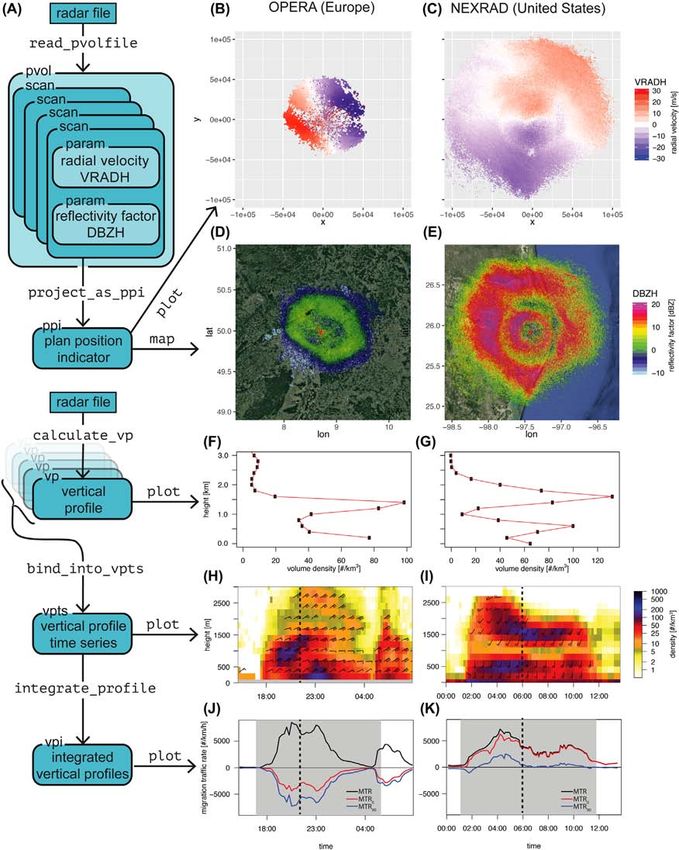
4Figure 2. The structure and interrelation of bioRad’s main class objects, functions, and plotting methods. (A) objects (rounded box), func-
tions (fixed width font) and their relation (arrows). (B–K) output of the default plot methods for a European radar (left row,
Offenthal radar, Germany, 2016-10-04 15:15 UTC–2016-10-05 08:45 UTC) and US radar (right row, KBRO radar, Texas, 2017-05-14
00:09 UTC–2017-05-14 13:25 UTC). The dotted line in (H) and (K) indicates the time slice of (B), (D), (F) and (C), (E), (J) respectively.
Figures (B) and (C) show radial velocity (VRADH) in m s–1 for the 1.5° elevation scans. Figures (D) and (E) show reflectivity factor
(DBZH) in dBZ for the same scans. Figure (F) and (G) shows animal density (dens) versus altitude (RCS = 11 cm2) for a single vertical
profile. Figure (H) and (I) show animal density (dens) and speed and direction (dd and ff) for a time series of vertical profiles. In figure
(J) and (K), black line shows MTR (migration traffic rate across a transect perpendicular to ground speed direction), blue line MTR0
(migration traffic rate across a fixed east-to-west transect) and red line MTR90 (migration traffic rate across a fixed north-to-south transect).
Grey shading indicates night time (time on the x-axis is in UTC). Altitudes are relative to mean sea level.
5TRUE will select default settings automatically (depending < sd_vvp_threshold. We recommend applying this
on radar wavelength and availability of polarimetric data). thresholding as a way of removing residual rain contamina-
We describe the most important algorithm parameters tions and insects in bird studies using C-band radars, where
and their preferred settings: sd_vvp_threshold = 2 m s–1 was shown a suitable value
1) range_min, range_max: sets the minimum and (Dokter et al. 2011). We note that sd_vvp may become
maximum range (distance from the radar) of data to include. large in relatively rare cases where the velocity field is highly
We recommend a minimum range of 5 km, to exclude the nonlinear (e.g. strong shear), causing this thresholding crite-
closest ranges that typically contain a lot of ground clut- rion to break down. For S-band radars VVP standard devia-
ter. We recommend a maximum range of 35 km, which tion thresholding has not been thoroughly evaluated, but
for most radars allows coverage up to 3 to 4 km a.s.l., radial velocity variability during bird migration may be lower
which is the altitude band in which most migration occurs than at C-band in certain cases. We currently recommend a
(Bruderer et al. 2018). At longer ranges, the radar beam gets conservative threshold of 1 m s–1 to retain more biological
very wide, hampering the radar’s ability to resolve altitudinal scatter.
distributions. 6) rcs: value for the radar cross section (RCS) of an
2) layers, layer_height: sets the number of individual. We recommend 11 cm2 as a starting point, which
altitude layers and their thickness, respectively. Altitudes are was the seasonal average for C-band radars in western Europe
defined relative to mean sea level, taking into account the during nocturnal passerine migration, according to a calibra-
antenna height as stored in the original polar volume file. We tion experiment (Dokter et al. 2011). Note that radar cross
recommend a thickness of 200 m. Profiles with narrower alti- sections depend on target size, body orientation, and radar
tude bin spacings can be extracted (Buler and Diehl 2009), wavelength (Vaughn 1985).
but the finite size of the radar beam precludes resolving altitu- The sd_vvp_threshold and rcs parameters can
dinal features smaller than approximately 100–200 m. Profile be changed using the sd_vvp_threshold and rcs
quantities are estimated based on resolution samples centered functions (in step 3 and up) without having to reprocess the
within the altitudinal spacing of each layer (Supplementary vertical profile (step 2).
material Appendix 1).
3) dual_pol, rho_hv: the logical dual_pol Step 3: visualizing and interpreting individual profiles
enables polarimetric filtering of precipitation, which discards The various quantities in a vertical profile (e.g. dens: ani-
contiguous areas with correlation coefficient (rHV) above a mal density, ff: ground speed, dd: ground speed direction,
threshold rho_hv. We recommend rho_hv = 0.95, since eta: reflectivity) can be visualized with plot, as shown in
precipitation typically has higher correlation coefficient Fig. 2F and 2G for density. These profile plots and Fig. 2D,
values (Stepanian et al. 2016) (but note that lower ρHV is pos- E are for the same moment in time. Note that both profiles
sible in mixed precipitation, like a combination of snow and show layering of birds: a density concentration at high alti-
rain, cf. Ryzhkov and Zrnic 1998). Single polarization mode tude (here at approx. 1.5 km) (cf. Dokter et al. 2013). These
is currently only available for C-band radars. layers show up as concentric rings in Fig. 2D and 2E. These
4) dealias, nyquist_min: the logical dealias rings appear because at an increasing distance from the radar,
enables radial velocity dealiasing following the method by measurements are made at higher altitudes, because of the
Haase and Landelius (2004) when scans are present with a positive beam elevation and the curvature of the earth.
Nyquist velocity smaller than threshold nyquist_min Also note that the peak densities of the two cases are simi-
(default 25 m s–1). The Nyquist velocity is stored in the lar, on the order of 100 individuals km–3 (assuming RCS = 11
attributes$how$NI slot of scan class objects. Some cm2) (Fig. 2H, I). The reflectivity factors (in dBZ scale,
radars dealias velocities at acquisition time, e.g. using the not to be confused with reflectivity η (Dokter et al. 2011,
dual-PRF technique (Holleman 2005). For such radars we Chilson et al. 2012b)) are however much higher for the US
recommend no dealiasing for scans on which this is applied. case than the European case. This is related to the difference
For data acquired with a single PRF we recommend dealias- in radar wavelength (Dokter et al. 2011), with NEXRAD
ing when the Nyquist velocity of a scan is below 25 m s–1, i.e. radars in the US being S-band and European radars being
if there is a high probability that animal movements will be mostly C-band.
faster than the Nyquist velocity.
5) sd_vvp_threshold: animal speed and direction Step 4: analyzing and visualizing vertical profiles as time
are estimated using the Volume Velocity Profiling (VVP) series
technique (Waldteufel and Corbin 1978, Holleman 2005). After processing volume data into profiles, the profile data of
VVP also provides the standard deviation of the fit residuals consecutive volume scans of a radar can be organized into a
(see Supplementary material Appendix 1, quantity sd_vvp time series of vertical profiles. The function bind_into_
in a profile). The sd_vvp_threshold parameter sets vpts binds vertical profile objects (class vp) into time series
the threshold for discarding data based on this stan- object (class vpts), for which the default plot is shown in
dard deviation measure. Animal density will be set to zero figure 2H and 2I. The dotted line indicates the time slice of
in altitude layers with a VVP standard deviation sd_vvp Fig. 2B–G.
6The plot method overlays one of the reflectivity-based Both the vp and vpts class objects can be exported to
quantities (e.g. dens, eta or dbz) with a barb indicating the standard R data frames (using as.data.frame) for fur-
animals ground speed and direction. This follows meteoro- ther analysis outside of bioRad.
logical conventions for graphically displaying wind speed and
direction (with north being up). The number of barb flags Conclusions, recommendations and outlook
indicate the speed (ff) while its tip points into the direction
where animals are moving (dd). bioRad provides a set of functions to extract biological infor-
Another useful profile quantity to inspect as time series is mation from weather radar data, to present the information
DBZH. This is the reflectivity factor for all scatterers, includ- in graphical form, and to aggregate it in useful summary sta-
ing meteorological targets like precipitation. Time periods tistics. bioRad streamlines the reporting of analysis results
with rain are often clearly visible as high DBZH values over according to existing conventions in the literature.
the full altitude column. We recommend making plots of For larger-bodied animals like birds, we recommend the
DBZH as a way of screening for precipitation contamina- following measures when reporting data in aggregated form:
tions and quality control, which is often a useful way to 1) To quantify the instantaneous intensity of migration,
check remarkable altitude patterns in the biological data (e.g. or other large-scale directed movements for which a rate of
the layering of birds at 1.5 km can also be seen in Fig. 2I) passage is of interest: MTR (if RCS unknown: RTR).
or short spikes with high values that might be due to rain 2) To quantify the number of migrants passing in a certain
contamination. time period: MT (if RCS unknown: RT).
bioRad provides multiple functions to further aggregate 3) To quantify the instantaneous number of animals aloft:
and summarize time series data. We can integrate over the VID (if RCS unknown: VIR). This measure is especially use-
altitude dimension using integrate_profile, which ful for cases that lack a large-scale directed movement, for
outputs a specially classed data.frame (class vpi) example at the moment of a synchronized exodus of flight
containing altitudinally integrated or averaged quantities (Shamoun-Baranes et al. 2011, Buler and Dawson 2014), or
(Fig. 1). Figure 2J and 2K show plots of migration traf- near a roost (Stepanian and Wainwright 2018).
fic rate, both MTR (variable transect angle, Eq. 1) and Traffic measures (MTR, RTR, MT, RT) can be condi-
MTR0 and MTR90 (fixed transect angle, Eq. 2). We note as tional on the choice of a transect line across which animals
before that MTR is always positive, but MTRα definitions are counted (angle α, cf. Eq. 2, 3). We therefore recommend
can become negative depending on the migratory direc- reporting whether a fixed transect was used or not, and if
tion in relation to α. For example, the northward spring so, its direction. These vertically-integrated quantities are also
migration (US case, Fig. 2K) result in a positive MTR0, conditional on an altitude band, therefore it should be clear
while the southward autumn migration (European case, whether they refer to the full altitude column, or only part
Fig. 2J) is negative. For the US case, migration is directed of it.
mostly northward, therefore MTR0 is much larger than The bioRad R software package aims to facilitate radar aer-
MTR90, while in the European case, migration is mostly oecology research and make weather radar a more accessible
westward, therefore (in absolute value) MTR0 is smaller tool in biological research to a broad range of researchers. We
than MTR90. encourage extending weather radar as a tool beyond its cur-
Vertically-integrated time series can be further accu- rent main application in quantifying songbird migration, e.g.
mulated in time into measures summarizing migra- towards larger flocking and soaring birds, bats and insects.
tion traffic having passed the radar station during a time Quantification of the movements of these species groups
period, like MT in Eq. 3 (cf. output columns mt and will require further calibration experiments (Dokter et al.
rt of integrate_profile). For example, for the 2011, Nilsson et al. 2019) and theoretical simulation work
European case we find MT = 55 × 103, MT0 = –28 × 103 (Mirkovic et al. 2016) to identify their radar signatures and
and MT90 = –45 × 103 for the time night-time period. validate quantifications, in which dual-polarization informa-
This means that – assuming a radar cross section (RCS) tion will likely be invaluable (Stepanian and Horton 2015,
per individual of 11 cm2 – 55 thousand birds per 1 km Stepanian et al. 2016). We also encourage the use of this
transect flew over the radar station in this night (irrespec- package in biological radar studies in other countries with
tive of direction). Decomposing the migration traffic into extensive weather radar networks, such as Australia, Canada,
two perpendicularly oriented components, we find a net 28 China, India, Japan and Russia, whose data might be read-
thousand birds flew southward per km over a west-to-east ily explored once converted to a standardized (OPERA or
transect (MT0), and a net 45 thousand birds per km flew NEXRAD) format. Expanding the use of weather radar net-
westward per km over a north-to-south transect (MT90). works for biological studies around the world will require
For these specific definitions, MT ≤ √(MT02 + MT902), with continuing improvements in access to data and standardiza-
the left- and right-hand side being equal when migration tion of data formats, and in raising awareness of the value
directions dd all point into a sector of at most 180 degrees of collecting, distributing and archiving clear-air biologi-
wide, as is usually the case for periods confined to a single cal data with radar operators. There is a broad potential for
spring or fall. using weather data in fundamental ecological research, in
7applications for mitigating wildlife-human conflicts, and Buler, J. J. and Dawson, D. K. 2014. Radar analysis of fall bird
in conservation (Bauer et al. 2017). We expect its use will migration stopover sites in the northeastern U.S. – Condor 116:
therefore only increase in the near future, and we hope these 357–370.
software tools will facilitate the further adoption of weather Chambers, J. M. 2016. Extending R. – Chapman and Hall/CRC.
radar in the toolkit of biologists, conservationists and policy Chilson, P. et al. 2012a. Partly cloudy with a chance of migration:
weather, radars, and aeroecology. – Bull. Am. Meteorol. Soc.
makers alike. 93: 669–686.
Chilson, P. et al. 2012b. Estimating animal densities in the aero-
Software availability sphere using weather radar: to Z or not to Z? – Ecosphere 3:
1–19.
bioRad’s homepage pro- Dokter, A. M. et al. 2011. Bird migration flight altitudes studied
vides links to R source code, install instructions, function by a network of operational weather radars. – J. R. Soc. Interface
documentation, vignettes and introductory exercises. 8: 30–43.
Software available on CRAN: and Github: . One 8: e52300.
Install latest release in R as install.packages(“bioRad”), and Dokter, A. M. et al. 2018. Seasonal abundance and survival of
latest development version as devtools::install_github(“adokter/ North America’s migratory avifauna determined by weather
bioRad”). radar. – Nat. Ecol. Evol. 2: 1603–1609.
Doviak, R. J. and Zrnić, D. S. 1993. Doppler radar and weather
C source code (vol2bird profiling algorithm) available observations. – Academic Press.
from: . Running Drake, V. A. et al. 2017. Ventral-aspect radar cross sections and
vol2bird in bioRad using calculate_vp() requires an instal- polarization patterns of insects at X band and their relation to
lation of Docker (linux, mac) or Docker for Windows size and form. – Int. J. Remote Sens. 38: 5022–5044.
(windows). Fijn, R. C. et al. 2015. Bird movements at rotor heights measured
License: MIT. continuously with vertical radar at a Dutch offshore wind farm.
To cite bioRad or acknowledge its use, cite this Software – Ibis 157: 558–566.
note as follows, substituting the version of the application Gasteren, H. Van et al. 2008. Extracting bird migration information
that you used for ‘version 0’: from C-band Doppler weather radars. – Ibis 150: 674–686.
Gauthreaux Jr, S. A. and Belser, C. G. 1998. Displays of bird move-
Dokter, A. M., Desmet, P., Spaaks, J. H., van Hoey, S., Veen, L., ments on the WSR-88D: patterns and quantification. – Weather
Verlinden, L., Nilsson, C., Haase, G., Leijnse, H., Farnsworth, Forecast. 13: 453–464.
A., Bouten, W. and Shamoun-Baranes, J. 2019. bioRad: Haase, G. and Landelius, T. 2004. Dealiasing of Doppler radar
biological analysis and visualization of weather radar data. velocities using a torus mapping. – J. Atmos. Ocean. Technol.
– Ecography 42: 000–000 (ver. 0). 21: 1566–1573.
Holleman, I. 2005. Quality control and verification of weather
radar wind profiles. – J. Atmos. Ocean. Technol. 22:
Funding – Funding received from Amazon Web Services, 1541–1550.
AWS Cloud Credits for Research (to AMD); National Science Horton, K. G. et al. 2014. A comparison of traffic estimates of
Foundation, Directorate for Biological Sciences, Division of nocturnal flying animals using radar, thermal imaging, and
Biological Infrastructure, no. 1661259; European Cooperation acoustic recording. – Ecol. Appl. 25: 390–401.
in Science and Technology, ESSEM COST Action ES1305 and Horton, K. G. et al. 2018. Navigating north: how body mass and
Netherlands Ministry of Defence, Bird Avoidance System (BAS). winds shape avian flight behaviors across a North American
migratory flyway. – Ecol. Lett. 21: 1055–1064.
Huuskonen, A. et al. 2014. The operational weather radar network
References in Europe. – Bull. Am. Meteorol. Soc. 95: 897–907.
Kahle, D. and Wickham, H. 2013. ggmap: spatial visualization
Ansari, S. et al. 2018. Unlocking the potential of NEXRAD data with ggplot2. – R J. 5: 144–161.
through NOAA’s Big Data Partnership. – Bull. Am. Meteorol. Lowery, G. H. 1951. A quantitative study of the nocturnal
Soc. 99: 189–204. migration of birds. – Univ. Kansas Publ. Mus. Nat. Hist. 3:
Bauer, S. et al. 2017. From agricultural benefits to aviation safety: 161–472.
realizing the potential of continent-wide radar networks. McLaren, J. D. et al. 2018. Artificial light confounds broad-
– BioScience 67: 912–918. scale habitat use by migrating birds. – Ecol. Lett. 21:
Bruderer, B. 1971. Radarbeobachtungen über den Frühlingszug im 356–364.
Schweizerischen Mittelland. – Ornithol. Beobachter 68: Michelson, D. 2014. EUMETNET OPERA weather radar
89–158. information model for implementation with the HDF5 file
Bruderer, B. et al. 2018. Vertical distribution of bird migration format, version 2.2. – EUMETNET OPERA Deliverable 38,
between the Baltic Sea and the Sahara. – J. Ornithol. 159: < http://eumetnet.eu/wp-content/uploads/2017/01/OPERA_
315–336. hdf_description_2014.pdf >.
Buler, J. J. and Diehl, R. H. 2009. Quantifying bird density during Mirkovic, D. et al. 2016. Electromagnetic model reliably predicts
migratory stopover using weather surveillance radar. – IEEE radar scattering characteristics of airborne organisms. – Sci.
Trans. Geosci. Remote Sens. 47: 2741–2751. Rep. 6: 1–11.
8Nilsson, et al. 2019. Revealing patterns of nocturnual migration using Stepanian, P. M. and Horton, K. G. 2015. Extracting migrant flight
the European weather radar network. – Ecography 42: xxx–xxx. orientation profiles using polarimetric radar. – IEEE Trans.
Rennie, S. J. 2014. Common orientation and layering of migrating Geosci. Remote Sens. 53: 6518–6528.
insects in southeastern Australia observed with a Doppler Stepanian, P. M. and Wainwright, C. E. 2018. Ongoing changes
weather radar. – Meteorol. Appl. 21: 218–229. in migration phenology and winter residency at Bracken Bat
Ryzhkov, A. V. and Zrnic, D. S. 1998. Discrimination between rain Cave. – Global Change Biol. 24: 3266–3275.
and snow with a polarimetric radar. – J. Appl. Meteorol. Stepanian, P. M. et al. 2016. Dual-polarization radar products for
Climatol. 37: 1228–1240. biological applications. – Ecosphere 7: e01539.
Schmaljohann, H. et al. 2008. Quantification of bird migration by Vaughn, C. R. 1985. Birds and insects as radar targets: a review.
radar – a detection probability problem. – Ibis 150: 342–355. – Proc. IEEE 73: 205–227.
Shamoun-Baranes, J. et al. 2011. Birds flee en mass from New Year’s Waldteufel, P. and Corbin, H. 1978. On the analysis of single-
Eve fireworks. – Behav. Ecol. 22: 1173–1177. Doppler radar data. – J. Appl. Meteorol. 18: 532–542.
Shamoun-Baranes, J. et al. 2014. Continental-scale radar monitor- Wickham, H. 2016. ggplot2: elegant graphics for data analysis.
ing of the aerial movements of animals. – Mov. Ecol. 2: 9. – Springer.
Supplementary material (Appendix ECOG-04028 at < www.
ecography.org/appendix/ecog-04028 >). Appendix 1.
9You can also read