Towards real-time probabilistic ash deposition forecasting for Aotearoa New Zealand
←
→
Page content transcription
If your browser does not render page correctly, please read the page content below
Towards real-time probabilistic ash deposition forecasting for Aotearoa New
Zealand
Rosa Trancoso
MetService
Yannik Behr ( y.behr@gns.cri.nz )
GNS Science
Tony Hurst
GNS Science
Natalia Deligne
United States Geological Survey
Method Article
Keywords: Volcanic hazard, ashfall, atmospheric models, HYSPLIT, ensembles, probabilistic forecast, Latin Hypercube, Aotearoa New Zealand, near real-time
forecasts
Posted Date: March 30th, 2022
DOI: https://doi.org/10.21203/rs.3.rs-1479358/v1
License: This work is licensed under a Creative Commons Attribution 4.0 International License. Read Full License
Page 1/17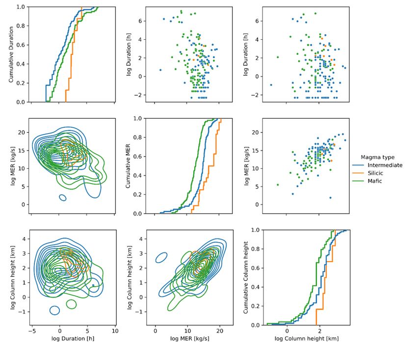
Abstract
Volcanic ashfall forecasts are highly dependent on eruption parameters and synoptic weather conditions at the time and location of the eruption. In
Aotearoa, New Zealand, MetService and GNS Science have been jointly developing an ashfall forecast system that incorporates 4D high-resolution numerical
weather prediction (NWP) and eruption parameters into the HYSPLIT model, a state-of-the art hybrid Eulerian and Lagrangian dispersion model widely used
for volcanic ash. However, these forecasts are based on discrete eruption parameters combined with a deterministic weather forecast and thus provide no
information on output uncertainty. This shortcoming hinders stakeholder decision making, particularly near the geographical margin of forecasted ashfall
and in areas with large gradients in forecasted ash deposition. This study presents a new approach that incorporates uncertainty from both eruptive and
meteorologic inputs to deliver uncertainty in the model output. To this end, we developed probabilistic density functions (PDFs) for the three key eruption
parameters (plume height, mass eruption rate, eruption duration) tailored to Aotearoa’s volcanoes, and combine them with NWP ensemble datasets to
generate probabilistic ashfall forecasts using the HYSPLIT model. We show that the Latin Hypercube Sampling (LHS) technique can be used to
representatively span this high-dimensional parameter space with fewer model runs than Monte Carlo techniques, thus allowing this methodology to be used
in near real-time forecast systems. We also propose new probabilistic summary products such as hazard matrices, probability of exceedance of cumulative
ashfall, and arrival time forecasting, which together support public information and emergency responders decision making.

Introduction
Explosive volcanic eruptions produce ash (glass, crystals, and rock particles < 2mm diameter) which can be carried hundreds of kilometres from the vent. It
can damage infrastructure and property, destroy crops, poison livestock, and pose serious risk for aviation and human health (Jenkins et al. 2015). Ash is
dispersed in the atmosphere and it remains there until it settles onto Earth’s surface (Carey and Bursik 2015). Besides tsunamis, volcanic eruptions are the
hazard with the largest footprint and the greatest social and economic impact (Wilson et al. 2015). Being so, ashfall and ash dispersion forecasts are the
most sought-after volcanic hazard information following an eruption (USGS 2022).

Where, when, and how much ash will be deposited depends on the type of eruption and the meteorological conditions. Only explosive eruptions will produce
significant amounts of ash and their size is typically described by the column height of the eruption plume, the duration of the eruption, the total or erupted
mass and the rate at which particles are ejected, the distribution of particles along the eruption column, and the grain size distribution of the erupted material
(Bonadonna et al. 2015). It often takes days to weeks to determine all these parameters following an eruption. To provide ashfall forecasts during the first
hours after an eruption, prior assumptions must be made for some or all the eruption parameters.

To address this problem, MetService, New Zealand's national weather authority and host of the Wellington Volcanic Ash Advisory Centre (VAAC), and GNS
Science, New Zealand’s provider of geological hazard information, have jointly developed an ashfall forecasting system for New Zealand’s 10 most active
volcanoes on or near the North Island (Fig. 1). This system combines discrete eruption scenarios provided by GNS Science for each of the volcanoes with 4D
high-resolution numerical weather prediction (NWP) provided by MetService, to generate forecast maps of ash depth on the ground (Hurst and Davis 2017).
The volcanic ash transport and deposition is computed with the HYSPLIT model, a state-of-the art hybrid Eulerian and Lagrangian dispersion model (Stein et
al. 2015a) used operationally by four of the nine VAACs (Prata and Rose 2015). The system produces updated forecasts every 6 hours, so that in case of an
eruption there is a preliminary forecast available.

However, because these forecasts are based on discrete eruption parameters combined with a deterministic weather forecast, they cannot capture the
breadth of possible outcomes and therefore provide no information on output uncertainty. Because uncertainty in the prior assumptions is large, it is critical
to quantify how they affect the forecasts.

Figure 2 demonstrates why quantifying uncertainties provides useful information to stakeholders as they assess mitigation options. For example, a
stakeholder might call for stronger mitigative actions if the forecast likelihood of exceeding a specified threshold is high, even if the expected value is low.

In this study, we aim to demonstrate a prototype system for a near real-time probabilistic ashfall forecasts in New Zealand, that accounts for both
uncertainties in eruption parameters and the current and future atmospheric state. Our method involves using the Latin Hypercube Sampling (LHS) technique
to representatively span this multidimensional parameter space with a reduced sample size, a critical consideration for a rapid response system. To achieve
this, we first compiled information and developed probability density functions (PDFs) for three key eruption source parameters (ESPs) – plume height, mass
eruption rate, eruption duration – tailored to Aotearoa’s volcanoes. Next, we combine these PDFs with NWP ensembles, using the LHS with Dependence, to
generate probabilistic ashfall forecasts with the HYSPLIT model.

Methodology
Uncertainty in eruption parameters

Quantifying uncertainty in the eruption parameters is challenging, particularly in the first hours of an eruption when reliable quantitative observations are
often not available (Aubry et al. 2021). Three key eruption source parameters (ESPs) for modelling volcanic ashfall transport are the eruption plume height
(H), mass eruption rate (MER), and eruption duration (D). Plume height is not trivial to reliably measure, can be variable on short timescales, and estimates
may have large uncertainties. The mass eruption rate is not directly measurable but usually derived from empirical correlations based on the observable
plume height, in relationships that have confidence intervals spanning orders of magnitude (Aubry et al. 2021; Mastin et al. 2009). Finally, eruption duration
is related to mass eruption rate and total volume erupted, and difficult to forecast while an eruption is ongoing. Existing data consists of a mix of directly
observed eruptions and derived estimates based on total ash erupted. What constitutes the ‘end’ of an eruption can also be difficult to ascertain.

                                                                           Page 2/17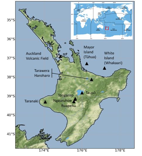
Volcano database and ESP PDFs

We undertook a comprehensive desktop study to develop, for the first time, PDFs for eruption plume height, the mass eruption rate, and eruption duration for
the 12 volcanic centres monitored by GeoNet (2022). The intention is to have a priori distributions ready to use if there is confirmation of an eruption. To
achieve this, we compiled a large dataset, combining datasets from Deligne (2021) and Aubry et al. (2021). We briefly describe both below.

Deligne (2021) compiled measured, estimated, and calculated estimates for volcanic eruption mass eruption rates, column heights, and durations from 213
events, a third of which are from New Zealand volcanoes. These include both prehistoric (estimates based on geologic record) and historic eruptions.
Eruptions were categorized according to magma type (mafic, intermediate, silicic) and eruption style (steam-driven, magmatic small to moderate, magmatic
large). Every entry was coded according to data type (e.g. instrumentally measured, observed, derived from geologic study) and assumptions made in
determining values. There was no attempt to evaluate the quality of the studies providing individual parameter values, nor an exclusion of derived values
(e.g. mass eruption rate is often calculated based on eruption column height, duration, and/or other parameters, but is rarely independently measured). For
this study, values compiled in Deligne (2021) derived from empirical or numerical models were removed.

Aubry et al. (2021) independently compiled estimates of total erupted mass of fall deposits, duration, eruption column height, and atmospheric conditions
from 134 eruptions from around the world from 1902–2016. Eruptions had to have independently measured/available values for all four parameters. Each
eruption was independently evaluated by at least two experts, and uncertainty associated with each parameter was systematically evaluated, with estimates
requiring a high degree of interpretation flagged.

For this study, we attributed magma type and eruption style categories using the criteria documented in Deligne (2021) to eruptions that solely appear in
Aubry et al. (2021). For 22 eruptions, there was no indication of eruption style apart from being classified as VEI 4 or smaller by the Smithsonian Global
Volcanism Program: we assigned these to the ‘Magmatic small to moderate’ eruption style category. Table 1 summarizes the collected data and Fig. 3 shows
the PDFs of ESPs by magma type.

                                                                           Table 1
                                               Summary of eruptions data compiled to estimate ESP distributions.
                                                Steam-driven      Magmatic small to moderate        Magmatic large   Total

                                Mafic           18 (7%)           78 (30%)                          4 (2%)           100 (38%)

                                Intermediate    27 (10%)          85 (33%)                          22 (8%)          134 (51%)

                                Silicic         1 (< 1%)          15 (6%)                           10 (4%)          26 (10%)

                                Total           46 (17%)          178 (69%)                         36 (14%)         260 (100%)

Uncertainty in weather

Uncertainty in weather is nowadays quantified with NWP ensemble datasets (Cheung 2001). These datasets seek to capture forecast error growth by running
many model realisations, with perturbed initial conditions that reflect uncertainty in the current atmospheric state, and perturbed model parameters that
reflect uncertainty in physical processes. The non-linear nature of the equations governing atmospheric motion means that even with perfectly known initial
conditions, the tiniest perturbations in atmospheric variables in the most accurate of NWP models may result in different outcomes after a finite time (Lorenz
1969; Zhang et al. 2019). The output of these ensembles is probabilistic, which more accurately reflects what is knowable about the future atmospheric state
than the deterministic picture provided by a single model.

NWP ensembles

The NWP ensemble datasets used in this study are from the Global Ensemble Forecast System version 12 (GEFSv12) running at the National Oceanic and
Atmospheric Administration (NOAA). The operational dataset is updated 4 times per day (cycles starting at 0, 6, 12 and 18:00 UTC) with 31 members (30
perturbed and 1 unperturbed/control) with approximately 25 km horizontal resolution and 64 vertical hybrid levels for atmospheric components, and out to
16 days of forecast at each cycle, except for 35 days at 0000 UTC (Stajner et al. 2020). The model output is public and available via NOMADS Server (2022)
at a 0.5° resolution grid, 3 hours temporal resolution, with surface and 12 pressure level fields up to 10 hPa, for the past 30 days.

We also made use of the historical dataset spanning from 2000–2019 consisting of GEFSv12 reforecasts (GENS-3), available via Open Data on AWS (2022)
but with only 21 members (20 perturbed and 1 unperturbed/control) available at a lower resolution (1° resolution grid and 6 hours temporal resolution) and
with less variables and less vertical levels (surface and 10 pressure level fields up to 10 hPa).

Combining uncertainties and sampling with Latin Hypercube technique

Multiple approaches can be taken to quantify uncertainty both from the source parameters as well as from the weather conditions. In our rapid response
context, the biggest challenge of probabilistic forecasting is to optimize resources while ensuring the spread and natural variability of our multidimensional
parameter space are well represented.

Monte Carlo sampling methods have been previously used in ash probabilistic forecasting (Hurst and Smith 2004; Magill et al. 2006) but they are only
computationally feasible with simplifying assumptions that limit the sample size. For instance, only using a few eruption sizes, and/or only using wind

                                                                             Page 3/17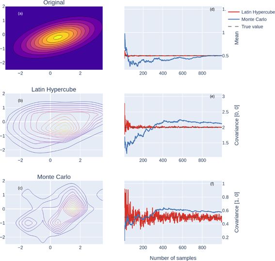
profiles at the vent location. While these assumptions may be reasonable for long-term hazard studies, they would likely result in inaccurate forecasts for a
single eruption and near real-time forecasting.

LHS is a stratified sampling approach that draws representative samples using a smaller sample size than Monte Carlo sampling, ensuring every section of
the parameter space is sampled once (Mckay et al. 2000). Sigg et al. (2018) and Prata et al. (2019) both used LHS techniques as an alternative to Monte
Carlo in dispersion applications. Sigg et al. (2018) considered a known amount of pollutant and the other LHS parameters were associated with microscale
boundary layer meteorology important for their specific small-scale application. Prata et al. (2019) considered large scale transport of airborne ash and
considered various eruption parameters as independent parameters in their LHS.

For our purposes, we considered the GEFSv12 ensemble dataset to be reliable in a statistical sense (i.e., over time, ensemble member counts of some
categorical weather event are consistent with their actual probability). The atmospheric evolution can be sampled by selecting an ensemble member, and as
we considered the eruption and atmospheric state to be independent, the ensemble member label can be considered an independent parameter with uniform
distribution (Stein et al. 2015b).

LHS with Dependence

The nature of the sampling problem for ESPs is different because they are not independent of each other – an underlying assumption of standard LHS
technique. To introduce correlation between ESPs, we assume that they approximately follow a multivariate Gaussian distribution (Packham and Schmidt
2008). We then first draw samples for each parameter from a standard Gaussian distribution x ∼ N(0,1) and then match the mean μ and covariance matrix
Σ of the prior eruption parameter distribution. Because we have three ESPs, x and μ are 3x1 vectors and Σ is a 3x3 matrix. A single LHS draw y can then be
expressed as:

y = Lx + μwithΣ = LL T Equation 1

where L is the Cholesky factorisation of Σ (Murphy 2022). It follows that y has the same mean as the original distribution. To see that y also has the same
covariance matrix we can calculate the covariance of y:

Cov(y) = LCov(x)L T = LIL T = Σ Equation 2

with I being the Identity matrix.

Figure 4 compares Monte Carlo and LHS techniques, demonstrating that LHS allows us to generate a representative sample of a given distribution with
considerably fewer samples than Monte-Carlo sampling requires.

LHS modelling runs

As previously mentioned, we considered each perturbed atmospheric state to be independent of each other and of the ESPs. To optimize computational
resources and maximize the weather variability information available, we constrained our ESP sample size to the same as the number of NWP ensembles,
(30 for GEFSv12 forecasts and 20 for GENS-3 reforecasts). Figure 5 shows that even a sample number of 20 suffices to have a good approximation to the
PDFs derived from historic eruptions (Fig. 3).

We then used these “eruption scenarios”, i.e., each point with a sampled MER, H, D and NWP ensemble member, to force independent ashfall dispersion
model runs, constraining H to a maximum of 20 km above mean sea level to fit within the weather forcing data, and D to a maximum of 24 hours which is
the forecast length. Table 2 summarizes the run parameters used as input to the dispersion model.

                                                                          Table 2
                                          HYSPLIT dispersion run parameters selected for each sample taken with LHS
                              Parameter                                         Sampling range

                              Plume height (H)                                  0–20 km above vent

                              Mass eruption rate (MER)                          Unconstrained

                              Eruption duration (D)                             0–24 h

                              Meteorological fields (Operational case study)    GEFSv12 members 1–30, 0.5° resolution, 3 hourly

                              Meteorological fields (Historical case study)     GENS-3 members 1–20, 1° resolution, 6 hourly
HYSPLIT configuration

Ashfall dispersion was computed with the HYSPLIT model version v5.0.1 (April 2020), a state-of-the art hybrid Eulerian and Lagrangian dispersion model
that is extensively used for volcanic ash transport and deposition by the international community (Rolph et al. 2017; Stein et al. 2015a).

The real and hypothetical eruptions studied here were located at Tongariro volcano (39.130 °S, 175.642 °E) with the main vent at 1978 m above sea level. It
typically erupts andesite lavas (Leonard et al. 2021), which we classified as “intermediate magma” in our eruption database (Table 1 and Fig. 3). The
configuration options used were implemented in Hurst and Davis (2017) and a brief description follows. The particle size distribution used for this volcano
was andesite with a density of 1300 kg/m3, divided into 37 size bins (see Fig. 6). The total mass erupted was distributed along the eruption column
according to a Suzuki distribution with constant 4 and discretized in 10 levels. This distribution adds more mass to the upper levels of the eruption plume, as
                                                                          Page 4/17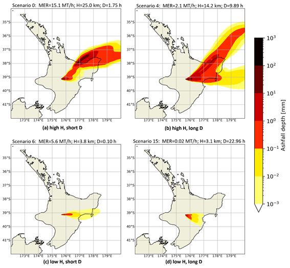
is typical for most eruptions (Suzuki 1983). Figure 7 shows the vertical plume mass profile for a sample of ESPs. Model results were integrated to a grid of 1
km horizontal resolution spanning 14 degrees latitude and longitude, from 48.5 °S to 33.5 °S and 165.5 °E to 180.5 °E.
Results
The proposed methodology was applied in two case studies that differ in the NWP forcing and LHS parameter sets.
The operational case study mimics a real-time eruption forecast at Tongariro, making use of the full set (30 members) of GEFSv12 forecasts routinely made
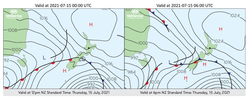
available by NOAA. We simulated a hypothetical eruption starting at 2021-07-15 00:00 UTC because during this day there was a wind shift near the volcano
centre (from south-westerly to westerly near Tongariro volcano – see Fig. 8) that allowed us to illustrate the importance of weather dynamics.
The historical case study refers to a past and well-studied eruption at Tongariro, starting at 2012-08-06 11:52:00 UTC (Hurst and Davis, 2017). In this case,
the available NWP forcing is from GENS-3, with less members (20 members) and lower spatial and temporal resolution than GEFSv12 forecasts. For this day,
the synoptic situation is quite different, with westerly winds that shift to north-westerly near the eruption as the front approaches New Zealand from the
Tasman Sea (Fig. 9).
Operational case study
The LHS parameters drawn for the operational case study are shown in Fig. 10. As mentioned before, each point of the sample is an “eruption scenario” -
corresponding to discrete values of MER, H, D and ensemble member - used to configure a HYSPLIT run. Each will produce a deterministic ashfall forecast
that can vary significantly from other ensemble members as can be seen in the deterministic examples in Fig. 11. Here, eruptions longer than 6 hours show
more dispersion to the west because of a wind shift from southwesterlies to westerlies around 6 hours after eruption. It is also interesting to note the clear
split on the ashfall footprint due to wind patterns affected by the mountainous terrain that crosses the North Island. The ash plume disperses either north or
south of the range, crossing it in its valleys if the wind is perpendicular (see terrain complexity on Fig. 1). This shows the importance of having a 4D NWP as
it accounts for terrain features.
Ensemble results are then summarized in products such as the ones presented below (Fig. 12 to Fig. 14). They allow us to see the probability of ashfall being
present in a location, when and how much. One of the most useful products for emergencies is the hazard matrix (Prata et al. 2019) that clearly shows the
areas that will be most likely affected by significant amounts of ash deposits. The comparison with a single ensemble member (blue contour in Fig. 12)
demonstrates the spread of the whole ensemble. For this case study eruption, only areas close to the volcano are likely (> 50%) to experience ashfall greater
than 1 mm or very likely (> 90%) to experience ashfall greater than 0.1 mm. A significant part of the ash deposits greater than 0.1 mm are likely to occur from
the source to the north-east, and then offshore. Most importantly, by accounting for the uncertainties in the eruption parameters and the NWP, a much wider
area is forecasted to possibly be affected by ashfall than if using only a single, deterministic forecast.
While Fig. 12 provides a concise summary of the whole ensemble forecast, Fig. 13 gives more detailed information on the probability of exceeding a given
threshold of ash deposits.
It is also useful to look at the arrival time of ash given the ensemble spread. Figure 14 shows the arrival time of the median probability of accumulated ash
thickness being higher than 0.01 mm (e.g. propagation in time of the 50% contour of the 0.01 mm exceedance probability). Here, the 0.01 mm threshold is
low enough to be considered as ash presence. While the forecast was produced for 24 hours, no more ash was deposited after 11 hours. This is consistent
with the 50% contour exceedance probability 0.01 mm after 24 h, shown in Fig. 13.
Historical case study
The LHS parameters drawn for the historical case study are shown in Fig. 15.
Analysing each simulation individually revealed that, for most scenarios, there’s an extremely narrow plume, as exemplified on the left-top image of Fig. 16,
which is consistent with results obtained by (Hurst and Davis, 2017, Fig. 6). For the scenarios with eruptions longer than 6 hours, there is a light plume
dispersion to the South, corresponding to the wind shifting from westerly to north-westerly as a front approaches (see scenarios 5, 10 and 13 with durations
of 7, 24 and 18h on Fig. 16 and synoptic conditions on Fig. 9). This southerly dispersion is however not significant enough to appear in the ensemble
summary products such as the hazard matrix, the exceedance probability, and arrival time products (Fig. 17 to Fig. 19). This fact clearly shows the power of
LHS for statistically meaningful probabilistic forecasts with reduced sample size, even in the absence of observations. Once observations were available, it
would be straightforward to redraw a new constrained LHS and trigger new HYSPLIT runs, thus reducing overall uncertainty while keeping the inherent
statistical variability.
Discussion
Results presented show how volcanic ash plume dispersion and deposition is highly dependent on the eruption parameters and the synoptic weather
conditions at the time and location of the eruption. As seen from the case studies, different plume heights and eruption durations from the same centre at the
same time can generate ash footprints in totally different regions, particularly if there is a shift in the wind direction. The timing and strength of a wind
variation (e.g. front arrival) is just one example of the phenomena subject to variability in a weather forecast, and only a physically-based 4D NWP ensemble
dataset can realistically cover the range of possibilities. It also highlights the importance of having realistic prior ESP distributions that cover pre-historic
eruptions. Large eruptions are likely to be underrepresented in historic catalogues which would lead to biases in the prior distributions.
Page 5/17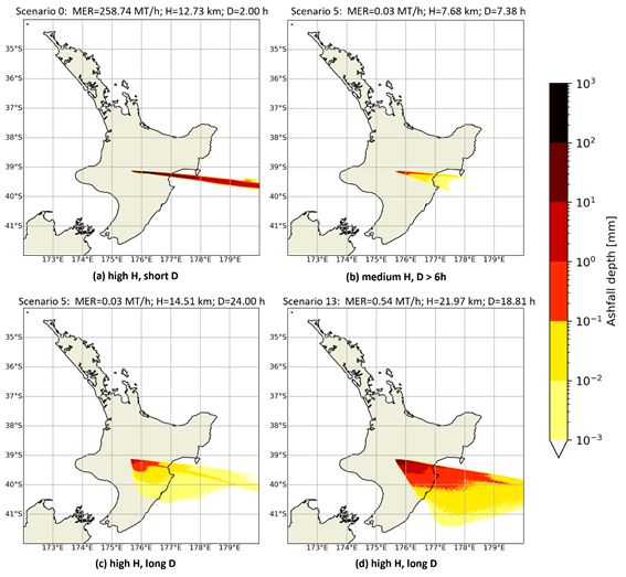
The historical case study shows the LHS technique allows incorporation of uncertainty to a forecast while keeping it within the observable range of
dispersion. It also reinforces us of the importance of updating information about ESP as soon as observations are made available, refining areas of
probability. Running the ensemble dispersion forecast a posteriori with refined ESPs can also incorporate more NWP sources, namely the ones with higher
resolution that are only available after the global models, overall leading to more accurate uncertainty estimation.

The number of ensemble members and spatial and temporal resolution of the forcing NWP are key factors in dispersion modelling, as can be seen from the
smoother gradients in maps for the operational case study when comparing to the historical case. In the future, as computational resources and global
ensembles become more accessible, dispersion runs could be forced by high-resolution NWP ensembles derived from the global datasets, using limited area
models such as WRF, extensively used at MetService.

Currently, the operational ashfall forecast system requires an expert to choose the most representative from the pre-computed scenarios. The proposed
methodology removes this need by having a prior distribution of ESPs rather than discrete scenarios. It comes however at the cost of significantly increased
computational resources. Using LHS is critical to keep the number of necessary forecast runs as low as possible in order to have a near real-time automated
system.

Conveying probabilistic results to non-experts can be challenging. Our results also allowed us to explore visual products that summarize the uncertainty
information in a concise manner and can hopefully be easily understood by end-users. The hazard matrix maps and probability of exceedance of cumulative
ash fall provide a summary picture of the situation after a certain time, while the ash arrival time map conveys the dynamic evolution that leads to the
previous products. Further stakeholder engagement will be required to find the best way of reporting probabilistic ashfall forecasts.

Conclusions
By quantifying uncertainty in ESPs, we have improved our understanding of Aotearoa volcanic eruptions and are able to provide uncertainty estimation to
ash dispersion input parameters. When combined with NWP ensemble datasets, we can also include variability in the weather forecast, which is key in any
probability dispersion forecast.

The method and results presented here shows that the LHS technique can be successfully used to representatively span the high dimensional parameter
space of combined uncertainty of ESPs and NWP, with a reduced sample size that allows for reasonable computational resources usage. This is a
determinant factor for a near real-time automated forecast system such as the one existing and developed in a joint effort between GNS Science and
MetService.

We also explored and propose visual products that summarize probabilistic forecast, such as the hazard matrix, probability of exceedance of cumulative ash
fall, and arrival time. These simpler but all-encompassing products can aid responding entities in selecting the most suitable mitigation action during a
volcanic crisis.

Future work could include quantifying uncertainty in other relevant ESPs, such as grain size distribution as it has a strong influence on ash deposition rates
and location. Furthermore, the ash dispersion run times could be optimized by dynamically adapting each model configuration to the eruption size.

Abbreviations
D – Eruption Duration

ESP – Eruption Source Parameters

GEFSv12 – Global Ensemble Forecast System version 12

GENS-3 – GEFSv12 reforecasts

H – Eruption Plume Height

LHS – Latin Hypercube Sampling

MER – Mass Eruption Rate

NOAA – National Oceanic and Atmospheric Administration, United States

NWP - Numerical Weather Prediction

PDF – Probability Distribution Function

VAAC – Volcanic Ash Advisory Centre

Declarations
Availability of data and materials
                                                                         Page 6/17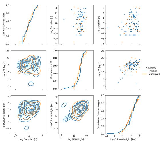
The scripts and dataset(s) supporting the conclusions of this article are available in the GitHub repository, https://github.com/yannikbehr/ashfall_forecasts
and Trancoso, R, Behr, Y, Hurst, T, & Deligne, N. (2022). HYSPLIT ensemble model output for case studies [Data set]. Zenodo.
https://doi.org/10.5281/zenodo.6363619

The HYSPLIT model used in this article was version 5.0.1 from https://www.ready.noaa.gov/index.php. The software is platform independent, based in
Fortran programming language and requires external NetCDF libraries. The source code for version 5.0.1 is not public and was made available to MetService
by the HYSPLIT developers. However, the most recent version of the model is available as pre-compiled binaries for multiple operating systems, to NOAA
users and registered HYSPLIT users.

Competing interests
The authors declare that they have no competing interests.

Funding
The work leading to this paper was funded by New Zealand Earthquake Commission (grant number EQC00035), GNS Science Core Funding, and MetService
Internal Funding.

Authors' contributions
    TH, ND and YB compiled and built PDFs for the volcanic ESP.
    YB implemented LHS technique with dependence
    RT collected and processed NWP data and ran the dispersion model experiments
    RT and YB explored and processed the model output into the final summary maps
    All authors drafted the manuscript.
    All authors read and approved the final manuscript.

Acknowledgements
The authors would like to thank Graham Rye, Principal Meteorological Developer at the Forecasting Research and Development group of MetService, for
providing the necessary setup on which to run the dispersion model on Amazon Web Services (AWS) as well invaluable guidance on how to better use
existing AWS resources for the current application.

The authors would like to also thank Cory Davis, previously working as Senior Research Scientist at the Forecasting Research and Development group of
MetService, for his invaluable contribution to ashfall forecasting in New Zealand and laying the foundations of the current work.

Authors' information (optional)

Affiliations
    MetService, New Zealand
         Rosa Trancoso
    GNS Science, New Zealand
         Yannik Behr, Tony Hurst
    United States Geological Survey, United States
         Natalia Deligne

Corresponding author
Correspondence to Yannik Behr (y.behr@gns.cri.nz)

References
  1. Aubry TJ, Engwell S, Bonadonna C, Carazzo G, Scollo S, Van Eaton AR, et al. The Independent Volcanic Eruption Source Parameter Archive (IVESPA,
    version 1.0): A new observational database to support explosive eruptive column model validation and development. Journal of Volcanology and
    Geothermal Research. 2021 Sep 1;417:107295.

                                                                         Page 7/17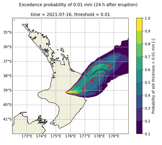
2. BOMS. BOMS Analysis Chart Archive [Internet]. corporateName = Bureau of Meteorology; 2022 [cited 2022 Mar 15]. Available from:
   http://www.bom.gov.au/australia/charts/archive/index.shtml
 3. Bonadonna C, Costa A, Folch A, Koyaguchi T. Chapter 33 - Tephra Dispersal and Sedimentation. In: Sigurdsson H, editor. The Encyclopedia of Volcanoes
   (Second Edition) [Internet]. Amsterdam: Academic Press; 2015 [cited 2022 Feb 2]. p. 587–97. Available from:
   https://www.sciencedirect.com/science/article/pii/B978012385938900033X
 4. Carey S, Bursik M. Chapter 32 - Volcanic Plumes. In: Sigurdsson H, editor. The Encyclopedia of Volcanoes (Second Edition) [Internet]. Amsterdam:
   Academic Press; 2015 [cited 2022 Feb 2]. p. 571–85. Available from: https://www.sciencedirect.com/science/article/pii/B9780123859389000328
 5. Cheung KKW. A review of ensemble forecasting techniques with a focus on tropical cyclone forecasting. Meteorological Applications. 2001;8(3):315–32.
 6. Deligne NI. Mass eruption rate, column height, and duration dataset for volcanic eruptions [Internet]. Mass eruption rate, column height, and duration
   dataset for volcanic eruptions. GNS Science; 2021. Available from: https://shop.gns.cri.nz/sr_2021-12-pdf/
 7. GeoNet. Geological Hazard Information for New Zealand. [Internet]. 2022 [cited 2022 Feb 14]. Available from: https://www.geonet.org.nz/
 8. Hurst T, Davis C. Forecasting volcanic ash deposition using HYSPLIT. Journal of Applied Volcanology. 2017 Mar 4;6(1):5.
 9. Hurst T, Smith W. A Monte Carlo methodology for modelling ashfall hazards. Journal of Volcanology and Geothermal Research. 2004 Dec
    15;138(3):393–403.
10. Jenkins S, Wilson T, Magill CR, Miller V, Stewart C, Blong R, et al. Volcanic ash fall hazard and risk. In: Loughlin S, Sparks S, Brown S, Jenkin S, Vye-
   Brown C, editors. Global Volcanic Hazards and Risk [Internet]. Cambridge: Cambridge University Press; 2015 [cited 2022 Feb 2]. Available from:
   https://research-information.bris.ac.uk/en/publications/volcanic-ash-fall-hazard-and-risk-2
11. Leonard GS, Cole RP, Christenson BW, Conway CE, Cronin SJ, Gamble J, et al. Ruapehu and Tongariro stratovolcanoes: a review of current
   understanding. Open Access Te Herenga Waka-Victoria University of Wellington; 2021 Jan 1 [cited 2022 Mar 15]; Available from:
   https://openaccess.wgtn.ac.nz/articles/journal_contribution/Ruapehu_and_Tongariro_stratovolcanoes_a_review_of_current_understanding/17128517/1
12. Lorenz EN. The predictability of a flow which possesses many scales of motion. Tellus. 1969;21(3):289–307.
13. Magill CR, Hurst AW, Hunter LJ, Blong RJ. Probabilistic tephra fall simulation for the Auckland Region, New Zealand. Journal of Volcanology and
   Geothermal Research. 2006 May 15;153(3):370–86.
14. Mastin LG, Guffanti M, Servranckx R, Webley P, Barsotti S, Dean K, et al. A multidisciplinary effort to assign realistic source parameters to models of
   volcanic ash-cloud transport and dispersion during eruptions. Journal of Volcanology and Geothermal Research. 2009 Sep 30;186(1):10–21.
15. Mckay MD, Beckman RJ, Conover WJ. A Comparison of Three Methods for Selecting Values of Input Variables in the Analysis of Output From a
   Computer Code. Technometrics. Taylor & Francis; 2000 Feb 1;42(1):55–61.
16. Murphy KP. Probabilistic Machine Learning: An introduction [Internet]. MIT Press; 2022 [cited 2022 Feb 3]. Available from: https://probml.github.io/pml-
   book/book1.html
17. NOMADS Server. NOMADS-NOAA Operational Model Archive and Distribution System [Internet]. 2022 [cited 2022 Feb 14]. Available from:
   https://nomads.ncep.noaa.gov/
18. Open Data on AWS. NOAA Global Ensemble Forecast System (GEFS) Re-forecast - Registry of Open Data on AWS [Internet]. 2022 [cited 2022 Feb 14].
   Available from: https://registry.opendata.aws/noaa-gefs-reforecast/
19. Packham N, Schmidt WM. Latin Hypercube Sampling with Dependence and Applications in Finance [Internet]. Rochester, NY: Social Science Research
    Network; 2008 Oct. Report No.: ID 1269633. Available from: https://papers.ssrn.com/abstract=1269633
20. Prata AT, Dacre HF, Irvine EA, Mathieu E, Shine KP, Clarkson RJ. Calculating and communicating ensemble-based volcanic ash dosage and concentration
   risk for aviation. Meteorological Applications. 2019;26(2):253–66.
21. Prata F, Rose B. Chapter 52 - Volcanic Ash Hazards to Aviation. In: Sigurdsson H, editor. The Encyclopedia of Volcanoes (Second Edition) [Internet].
   Amsterdam: Academic Press; 2015 [cited 2022 Feb 3]. p. 911–34. Available from:
   https://www.sciencedirect.com/science/article/pii/B9780123859389000523
22. Rolph G, Stein A, Stunder B. Real-time Environmental Applications and Display sYstem: READY. Environmental Modelling & Software. 2017 Sep
    1;95:210–28.
23. Sigg R, Lindgren P, von Schoenberg P, Persson L, Burman J, Grahn H, et al. Hazmat risk area assessment by atmospheric dispersion modelling using
   Latin hypercube sampling with weather ensemble. Meteorological Applications. 2018;25(4):575–85.
24. Stajner I, Tallapragada V, Zhu Y, Alves H, McQueen J, Hamill T, et al. NOAA’s unified forecast System for sub-seasonal predictions: Development and
   operational implementation plans of Global Ensemble Forecast System v12 (GEFSv12) at NCEP [Internet]. Copernicus Meetings; 2020 Mar. Report No.:
   EGU2020-6212. Available from: https://meetingorganizer.copernicus.org/EGU2020/EGU2020-6212.html
25. Stein AF, Draxler RR, Rolph GD, Stunder BJB, Cohen MD, Ngan F. NOAA’s HYSPLIT Atmospheric Transport and Dispersion Modeling System. Bulletin of
   the American Meteorological Society. American Meteorological Society; 2015a Dec 1;96(12):2059–77.
26. Stein AF, Ngan F, Draxler RR, Chai T. Potential Use of Transport and Dispersion Model Ensembles for Forecasting Applications. Weather and Forecasting.
   American Meteorological Society; 2015b Jun 1;30(3):639–55.
27. Suzuki T. A Theoretical Model for Dispersion of Tephra. Arc volcanism: physics and tectonics [Internet]. Shimozuru, D., Yokohama, I. Tokyo: Terra
   Scientific Publishing; 1983. p. 95–113. Available from:
   https://pages.mtu.edu/~raman/Ashfall/Syllabus/Entries/2009/6/21_Ash_Blankets_files/Suzuki83.pdf

                                                                          Page 8/17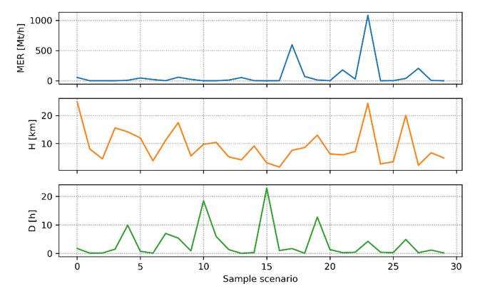
28. USGS. Volcanic Ash Impacts & Mitigation - Volcanic Ash Impacts & Mitigation [Internet]. 2022 [cited 2022 Feb 27]. Available from:
    https://volcanoes.usgs.gov/volcanic_ash/
29. Wilson TM, Jenkins S, Stewart C. Chapter 3 - Impacts from Volcanic Ash Fall. In: Shroder JF, Papale P, editors. Volcanic Hazards, Risks and Disasters
    [Internet]. Boston: Elsevier; 2015 [cited 2022 Feb 2]. p. 47–86. Available from:
    https://www.sciencedirect.com/science/article/pii/B9780123964533000034
30. Zhang F, Sun YQ, Magnusson L, Buizza R, Lin S-J, Chen J-H, et al. What Is the Predictability Limit of Midlatitude Weather? Journal of the Atmospheric
    Sciences. American Meteorological Society; 2019 Apr 1;76(4):1077–91.

Figures

Figure 1

New Zealand 10 volcanic centres for which ashfall forecasts are routinely generated (black triangles). Inlet world map shows International VAAC regions
(MetService hosts VAAC Wellington) with a red dashed box around North Island of New Zealand for location.

Figure 2

PDFs illustrating the importance of providing uncertainty estimates: there is a greater probability that scenario 1 exceeds a critical threshold despite having a
lower estimated value than scenario 2. Source: adapted from Sigg et al. (2018)

                                                                          Page 9/17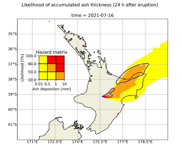
Figure 3

Logarithmic ESP distributions coloured by magma type. From top to bottom rows: Duration [h], Mass eruption rate [kg/s] and Column height above vent [km].
The diagonal panels show the empirical cumulative distribution functions; upper triangular panels show the distributions between pairs of ESPs; lower
triangular panels show the same distributions interpolated using kernel density estimation.

                                                                        Page 10/17
Figure 4
Performance of Monte Carlo and LHS techniques as a function of number of samples. a) shows the 2D Gaussian distribution from which samples are
drawn; b) and c) show the LHS and Monte Carlo estimate, respectively, from 20 random samples. d) to f) show the evolution of the estimates of first and
second moment for LHS and Monte Carlo samples with respect to the number of samples.
Figure 5
Comparison of original (blue) and LHS resampled (orange) distribution of ESP for 20 samples and intermediate magma (see Figure 3).
Page 11/17Figure 6
Particle size distribution for andesitic ash (density 1300 kg/m3). Source: Hurst and Davis (2017).
Figure 7
Vertical distribution of eruption plume mass for a set of ESPs.
Page 12/17Figure 8
Synoptic weather evolution for the operational case study. Black contours are isobars at mean sea level. Black star is Tongariro volcanic centre. Source:
MetService Internal Archive
Figure 9
Synoptic weather evolution for the historical case study. Black contours are isobars at mean sea level. Black star is Tongariro volcanic centre. Source: BOMS
(2022)
Page 13/17Figure 10
LHS draw with 30 points used in the operational case study. From top to bottom: mass eruption rate (MER), eruption column height above vent (H), and
eruption duration (D).
Figure 11
Example of deterministic ashfall forecasts for 4 points of the LHS sample (each point is a set of ESPs and ensemble member). The points were chosen to
show variability.
Figure 12
Cumulative ashfall hazard map color-coding areas by the likelihood of ashfall exceeding a given threshold (see inset matrix for details) for a forecast 24
hours after eruption. The blue line shows the contour of the 0.01 mm deposition for a single ensemble member.
Page 14/17Figure 13
Probability of cumulative ashfall exceeding 0.01 mm, for a forecast 24 hours after eruption. The red line shows the median (50%) probability.
Figure 14
Propagation in time of the median probability shown in Figure 13 in one-hour steps for a forecast 24 hours after eruption. Most ash falls within 9 hours after
eruption.
Page 15/17Figure 15
LHS draw with 20 points used in the historical case study. From top to bottom: mass eruption rate (MER), eruption column height above vent (H), and
eruption duration (D) as for Figure 10.
Figure 16
Example of deterministic ashfall forecasts for 4 points of the Latin Hypercube sample (each point is a set of ESPs and ensemble member). The points were
chosen to show variability.
Figure 17
Cumulative ashfall hazard map color-coding areas by the likelihood of ashfall exceeding a given threshold (see inset matrix for details) for a forecast 24
hours after eruption. The blue line shows the contour of the 0.01 mm deposition for a single ensemble member.
Figure 18
Probability of cumulative ashfall exceeding 0.01 mm for a forecast 24 hours after eruption. The red line shows the median (50%) probability.
Page 16/17Figure 19
Propagation in time of the median probability shown in Figure 18 in one-hour steps for a forecast 24 hours after eruption. Most ash falls within 7-8 hours
after eruption.
Page 17/17You can also read