We are More than Our Joints: Predicting how 3D Bodies Move - arXiv.org
←
→
Page content transcription
If your browser does not render page correctly, please read the page content below
We are More than Our Joints: Predicting how 3D Bodies Move

                                                                        Yan Zhang1 , Michael J. Black2 , Siyu Tang1
                                                                                  1
                                                                                    ETH Zürich, Switzerland
                                                              2
                                                                Max Planck Institute for Intelligent Systems, Tübingen, Germany
arXiv:2012.00619v2 [cs.CV] 2 Apr 2021

                                        Figure 1: We represent the body in motion with a set of 3D markers on the body surface. Given a time sequence of markers
                                        from the past (white), MOJO predicts diverse marker sequences in the future (orange) with 3D bodies they represent (gray).

                                                                Abstract                               tent DCT space that generates motions from latent frequen-
                                                                                                       cies. MOJO preserves the full temporal resolution of the
                                           A key step towards understanding human behavior is the      input motion, and sampling from the latent frequencies ex-
                                        prediction of 3D human motion. Successful solutions have       plicitly introduces high-frequency components into the gen-
                                        many applications in human tracking, HCI, and graphics.        erated motion. We note that motion prediction methods ac-
                                        Most previous work focuses on predicting a time series of      cumulate errors over time, resulting in joints or markers
                                        future 3D joint locations given a sequence 3D joints from      that diverge from true human bodies. To address this, we
                                        the past. This Euclidean formulation generally works bet-      fit the SMPL-X body model to the predictions at each time
                                        ter than predicting pose in terms of joint rotations. Body     step, projecting the solution back onto the space of valid
                                        joint locations, however, do not fully constrain 3D human      bodies, before propagating the new markers in time. Quan-
                                        pose, leaving degrees of freedom (like rotation about a        titative and qualitative experiments show that our approach
                                        limb) undefined. Note that 3D joints can be viewed as a        produces state-of-the-art results and realistic 3D body an-
                                        sparse point cloud. Thus the problem of human motion           imations. The code is available for research purposes at
                                        prediction can be seen as a problem of point cloud pre-        https://yz-cnsdqz.github.io/MOJO/MOJO.html.
                                        diction. With this observation, we instead predict a sparse
                                        set of locations on the body surface that correspond to mo-    1. Introduction
                                        tion capture markers. Given such markers, we fit a para-
                                        metric body model to recover the 3D body of the person.           Human motion prediction has been extensively studied
                                        These sparse surface markers also carry detailed informa-      as a way to understand and model human behavior. Pro-
                                        tion about human movement that is not present in the joints,   vided the recent past motion of a person, the goal is to pre-
                                        increasing the naturalness of the predicted motions. Us-       dict either a deterministic or diverse set of plausible motions
                                        ing the AMASS dataset, we train MOJO (More than Our            in the near future. While useful for animation, AR, and
                                        JOints), which is a novel variational autoencoder with a la-   VR, predicting human movement is much more valuable be-
cause it means we have a model of how people move. Such           quency bands in the latent space via a discrete cosine trans-
a model is useful for applications in sports [60], pedestrian     form (DCT). Based on the energy compaction property of
tracking [47], smart user interfaces [54], robotics [31] and      the DCT [3, 45]1 , we train our CVAE with a robust Kull-
more. While this is a variant of the well-studied time-series     back–Leibler divergence (KLD) term [61], creating an im-
prediction problem, most existing methods are still not able      plicit latent prior that carries most of the information at low
to produce realistic 3D body motion.                              frequency bands. To sample from this implicit latent prior,
   To address the gap in realism, we make several novel           we employ diversifying latent flows (DLows) [57] in low-
contributions but start with a few observations. First, most      frequency bands to produce informative features, and from
existing methods for 3D motion prediction treat the body as       the standard normal distribution in high-frequency bands to
a skeleton and predict a small set of 3D joints. While some       produce white noise. Pieces of information from various
methods represent the skeleton in terms of joint angles, the      frequencies are then fused to compose the output motion.
most accurate methods simply predict the 3D joint locations           Third, in the inference phase, we propose a recursive pro-
in Euclidean space. Second, given a sparse set of joint loca-     jection scheme supported by our marker-based representa-
tions, animating a full 3D body is ambiguous because im-          tion, in order to retain natural body shape and pose through-
portant degrees of freedom are not modeled, e.g. rotation         out the sequence. We regard the valid body space as a low-
about limb axes. Third, most papers show qualitative re-          dimensional manifold in the Euclidean space of markers.
sults by rendering skeletons and these often look fine to the     When the CVAE decoder makes a prediction step, the pre-
human eye. We show, however, that, as time progresses,            dicted markers tend to leave this manifold because of error
the skeletons can become less and less human in proportion        accumulation. Therefore, after each step we project the pre-
so that, at the end of the sequence, the skeleton rarely corre-   dicted markers back to the valid body manifold, by fitting
sponds to a valid human body. Fourth, the joints of the body      an expressive SMPL-X [41] body mesh to the markers. On
cannot capture the nuanced details of how the surface of the      the fitted body, we know the true marker locations and pass
body moves, limiting realism of any resulting animation.          these to the next stage of the RNN, effectively denoising the
   We address these issues with a solution, called MOJO           markers at each time instant. Besides keeping the solution
(More than Our JOints) the predicts realistic 3D body mo-         valid, the recursive projection scheme directly yields body
tion. MOJO incorporates a novel representation of the body        model parameters and hence realistic body meshes.
in motion, a novel motion generative network, and a novel             We exploit the AMASS [34] dataset for evaluation, as
scheme for 3D body mesh recovery.                                 well as Human3.6M [25] and HumanEva-I [48] to com-
   First, the set of 3D joints predicted by existing methods      pare our methods with the state-of-the-art in stochastic mo-
can be viewed as a sparse point cloud. In this light, existing    tion prediction. We show that our models with the latent
human motion prediction methods preform point cloud pre-          DCT space outperform the state-of-the-art, and that the re-
diction. Thus, we are free to choose a different point cloud      cursive projection scheme effectively eliminates unrealistic
that better satisfies the ultimate goal of animating bodies.      body deformation. We also evaluate realism of the gener-
Specifically, we model the body with a sparse set of sur-         ated motion with a foot skating measure and a perceptual
face markers corresponding to those used in motion capture        study. Finally, we compare different body representations,
(mocap) systems. We simply swap one type of sparse point          in particular our solution with a traditional pipeline, which
cloud for another, but, as we will show, predicting surface       first predicts 3D joints and then fits a body to the joints.
markers has key advantages. For example, there exist meth-        We find that they are comparable w.r.t. prediction diversity
ods to fit a SMPL body model [33] to such makers, produc-         and accuracy, but the traditional pipeline can produce in-
ing realistic animations [32, 34]. Consequently this shift        valid body shapes.
to predicting makers enables us to (1) leverage a powerful        Contributions. In summary, our contributions are: (1) We
statistical body shape model to improve results, (2) imme-        propose a marker-based representation for bodies in mo-
diately gives us realistic animations, (3) provides an output     tion, which provides more constraints than the body skele-
representation that can be used in many applications.             ton and hence benefits 3D body recovery. (2) We design
   Second, to model fine-grained and high-frequency in-           a new CVAE with a latent DCT space to improve motion
teractions between markers, we design a conditional vari-         modelling. (3) We propose a recursive projection scheme to
ational autoencoder (CVAE) with a latent cosine space. It         preserve valid bodies at test time.
not only performs stochastic motion prediction, but also im-
proves motion realism by incorporating high-frequency mo-         2. Related Work
tion details. Compared to most existing methods that en-             Deterministic human motion prediction. Given an in-
code motion with a single vector (e.g. the last hidden state      put human motion sequence, the goal is to forecast a de-
of an RNN), our model preserves full temporal resolution of
the sequence, and decomposes motion into independent fre-           1 Most   information will be concentrated at low frequency bands.
terministic future motion, which is expected to be close          produced and the pose sequence is then generated. Zhang
to the ground truth. This task has been extensively stud-         et al. [61] represent the body in motion by the 3D global
ied [5, 6, 10, 13, 15, 16, 17, 18, 28, 29, 35, 36, 42, 43, 49,    translation and the joint rotations following the SMPL kine-
51, 63]. Martinez et al. [36] propose an RNN with resid-          matic tree [33]. When animating a body mesh, a constant
ual connections linking the input and the output, and design      body shape is added during testing. Although a constant
a sampling-based loss to compensate for prediction errors         body shape is preserved, foot skating frequently occurs due
during training. Cai et al. [10] and Mao et al. [35] use the      to the inconsistent relation between the body pose, the body
discrete cosine transform (DCT) to convert the motion into        shape and the global translation.
the frequency domain. Then Mao et al. [35] employ graph               MOJO in context. Our solution not only improves
convolutions to process the frequency components, whereas         stochastic motion prediction over the state-of-the-art, but
Cai et al. [10] use a transformer-based architecture.             also directly produces diverse future motions of realistic 3D
    Stochastic 3D human motion prediction. In contrast            bodies. Specifically, our latent DCT space represents mo-
to deterministic motion prediction, stochastic motion pre-        tion with different frequencies, rather than a single vector
diction produces diverse plausible future motions, given a        in the latent space. We find that generating motions from
single motion from the past [7, 8, 14, 19, 30, 50, 56, 57, 61].   different frequency bands significantly improves diversity
Yan et al. [56] propose a motion transformation VAE to            while retaining accuracy. Additionally, compared to previ-
jointly learn the motion mode feature and transition be-          ous skeleton-based body representations, we propose to use
tween motion modes. Barsoum et al. [7] propose a proba-           markers on the body surface to provide more constraints on
bilistic sequence-to-sequence model, which is trained with a      the body shape and DoFs. This marker-based representation
Wasserstein generative adversarial network. Bhattacharyya         enables us to design an efficient recursive projection scheme
et al. [8] design a ‘best-of-many’ sampling objective to          by fitting SMPL-X [41] at each prediction step. Recently,
boost the performance of conditional VAEs. Gurumurthy et          in the context of autonomous driving, Weng et al. [52, 53]
al. [19] propose a GAN-based network and parameterize the         forecast future LiDAR point clouds and then detect-and-
latent generative space as a mixture model. Yuan et al. [57]      track 3D objects in the predicted clouds. While this has
propose diversifying latent flows (DLow) to exploit the la-       similarities to MOJO, they do not address articulated hu-
tent space of an RNN-based VAE, which generates highly            man movements.
diverse but accurate future motions.
    Frequency-based motion analysis. Earlier studies like         3. Method
[38, 44] adopt a Fourier transform for motion synthesis and       3.1. Preliminaries
tracking. Akhter et al. [4] propose a linear basis model
for spatiotemporal motion regularization, and discover that       SMPL-X body mesh model [41]. Given a compact set of
the optimal PCA basis of a large set of facial motion con-        body parameters, SMPL-X produces a realistic body mesh
verges to the DCT basis. Huang et al. [24] employ low-            including face and hand details. In our work, the body pa-
frequency DCT bands to regularize motion of body meshes           rameter set Θ includes the global translation t ∈ R3 , the
recovered from 2D body joints and silhouettes. The studies        global orientation R ∈ R6 w.r.t. the continuous repre-
of [10, 35, 51] use deep neural networks to process DCT fre-      sentation [62], the body shape β ∈ R10 , the body pose
quency components for motion prediction. Yumer et al. [59]        θ ∈ R32 in the VPoser latent space [41], and the hand pose
and Holden et al. [23] handle human motions in the Fourier        θ h ∈ R24 in the MANO [46] PCA space. We denote a
domain to conduct motion style transfer.                          SMPL-X mesh as M(Θ), which has a fixed topology with
    Representing human bodies in motion. 3D joint loca-           10,475 vertices. MOJO is implemented using SMPL-X in
tions are widely used, e.g. [29, 36, 57]. To improve predic-      our work, but any other parametric 3D body model could be
tion accuracy, Mao et al. [35], Cui et al. [13], Li et al. [29]   used, e.g. [39, 55].
and others use a graph to capture interaction between joints.     Diversifying latent flows (DLow) [57]. The entire DLow
Askan et al. [6] propose a structured network layer to repre-     method comprises a CVAE to predict future motions, and
sent the body joints according to a kinematic tree. Despite       a network Q that takes the condition sequence as input and
their effectiveness, the skeletal bone lengths can vary dur-      transforms a sample ε ∼ N (0, I) to K diverse places in
ing motion. To alleviate this issue, Hernandez et al. [22]        the latent space. To train the CVAE, the loss consists of a
use a training loss to penalize bone length variations. Gui       frame-wise reconstruction term, a term to penalize the dif-
et al. [17] design a geodesic loss and two discriminators         ference between the last input frame and the first predicted
to keep the predicted motion human-like over time. To re-         frame, and a KLD term. Training the network Q requires a
move the influence of body shape, Pavllo et al. [42, 43] use      pre-trained CVAE decoder, their training loss encourages
quaternion-based joint rotations to represent the body pose.      diverse generated motion samples in which, at least one
When predicting the global motion, a walking path is first        sample is close to the ground truth motion.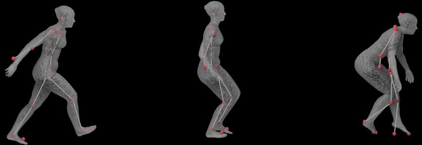
to model motions at different granularity levels.
                   condition module    encoder         decoder
                                                                         Architectures. Our model is visualized in Fig. 2, which is
         GRU                          fc
                                                                         designed according to the CVAE in the DLow method [57].
                                                                         The encoder with a GRU [12] preserves full temporal reso-
         GRU   c         fc      1

                                           c     GRU     fc      +       lution of the input. Then, the motion information is decom-
                                      I
                     D
                                      D
                                                                         posed onto multiple frequency bands via DCT. At individual
         GRU   c     C   fc                c     GRU     fc      +       frequency bands, we use the re-parameterization trick [26]
                                 1

                                      C
                     T
                                      T                                  to introduce randomness, and then use inverse DCT to con-
         GRU   c         fc      1

                                           c     GRU     fc      +
                                                                         vert the motion back to the temporal domain. To improve
  …

                                                                     …
                                …

                                                  …
          …

                                                                         temporal smoothness and eliminate the first-frame jump re-
Figure 2: Illustration of our CVAE architecture. The red                 ported in [36], we use residual connections at the output.
arrows denote sampling from the inference posterior. The                 We note that the CVAE in the DLow method, which does
circles with ‘c’ and ‘+’ denote feature concatenation and                not have residual connections but has a loss to penalize the
addition, respectively. The blocks with ‘fc’ denote a stack              jump artifact, does not produce smooth and realistic marker
of fully-connected layers.                                               motions. A visualization of this latent DCT space is shown
                                                                         in the Appendix.
                                                                         Training with robust Kullback-Leibler divergence. Our
3.2. Human Motion Representation
                                                                         training loss comprises three terms for frame-wise recon-
    Most existing methods use 3D joint locations or rotations            struction, frame-wise velocity reconstruction, and latent
to represent the body in motion. This results in ambiguities             distribution regularization, respectively;
in recovering the full shape and pose [9, 41]. To obtain
                                                                            L = EY [|Y − Y rec |] + αEY [|∆ Y − ∆ Y rec |]
more constraints on the body, while preserving efficiency,                                                                         (1)
we represent bodies in motion with markers on the body                         + Ψ (KLD(q(Z|X, Y )||N (0, I)))) ,
surface. Inspired by modern mocap systems, we follow the                 where the operation ∆ computes the time difference, q(·|·)
marker placements of either the CMU mocap dataset [1] or                 denotes the inference posterior (the encoder), Z denotes the
the SSM2 dataset [34], and select V vertices on the SMPL-                latent frequency components, and α is a loss weight. We
X body mesh, which are illustrated in the Appendix.                      find the velocity reconstruction term can further improve
    The 3D markers are simply points in Euclidean space.                 temporal smoothness.
Compared to representing the body with the global transla-                   Noticeably, our distribution regularization  term is given
                                                                                                                    √
tion and the local pose, like in [43, 61], such a location-              by the robust KLD [61] with Ψ(s) = 1 + s2 − 1 [11],
based representation naturally couples the global body                   which defines an implicit latent prior different from the
translation and the local pose variation, and hence is less              standard normal distribution. During optimization, the gra-
prone to motion artifacts like foot skating, which are caused            dients to update the entire KLD term become smaller when
by the mismatch between the global movement, the pose                    the divergence from N (0, I) becomes smaller. Thus, it
variation, and the body shape.                                           expects the inference posterior to carry information, and
    Therefore, in each frame the body is represented by a                prevents posterior collapse. More importantly, this term
V-dimensional feature vector, i.e. the concatenation of the              is highly suitable for our latent DCT space. According to
3D locations of the markers, and the motion is represented               the energy compaction property of DCT [3, 45], we expect
by a time sequence of such vectors. We denote the in-                    that the latent prior deviates from N (0, I) at low-frequency
put sequence to the model as X := {xt }M      t=0 , and a pre-           bands to carry information, but equals N (0, I) at high-
dicted future sequence from the model as Y := {yt }N      t=0 ,          frequency bands to produce white noise. We let this robust
where y0 = xM +1 . With fitting algorithms like MoSh and                 KLD term determine which frequency bands to carry infor-
MoSh++ [32, 34], it is much easier to recover 3D bodies                  mation automatically.
from markers than from joints.                                           Sampling from the latent DCT space. Since our latent
                                                                         prior is implicit, sampling from the latent space is not as
3.3. Motion Generator with Latent Frequencies
                                                                         straightforward as sampling from the standard normal dis-
   For a real human body, the motion granularity usually                 tribution, like for most VAEs. Due to the DCT nature,
corresponds to the motion frequency because of the un-                   we are aware that motion information is concentrated at
derlying locomotor system. For example, the frequency of                 low-frequency bands, and hence we directly explore these
waving hands is usually much higher than the frequency of a              informative low-frequency bands using the network Q in
jogging gait. Therefore, we design a network with multiple               DLow [57].
frequency bands in the latent space, so as to better repre-                  Specifically, we use {Qw }L w=1 to sample from the lowest
sent interactions between markers on the body surface and                L frequency bands, and sample from N (0, I) from L + 1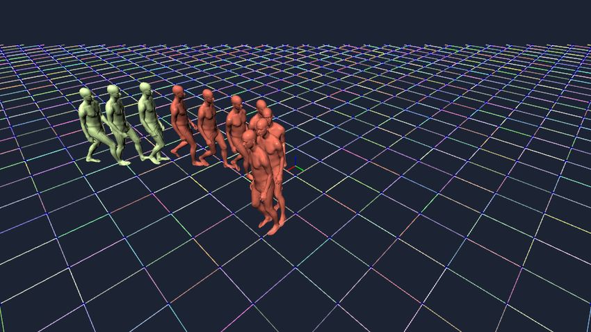
(1) optimizing the global configurations t and R, (2) ad-
                                           condition module         DLow         decoder
                                                                                            ditionally optimizing the body pose θ, and (3) additionally
                       GRU                               fc                                 optimizing the hand pose θ h . At each time t, we use the
                                                                                            previous fitted result to initialize the current optimization
                                                                                            process, so that the optimum can be reached with a small
   {Qw}                  {Tw}j                                    VAE Decoder
  w=0,1,..,L-1         w=0,1,..,L-1
                                                                                            number of iterations. The loss of our optimization-based
                                                                                j=1,2,…,K
                                                                                            fitting at time t is given by

Figure 3: Illustration of our sampling scheme to generate                                    Lf (Θt ) := |VM(Θt ) − ytpred |2 + λ1 |θt |2 + λ2 |θth |2 , (2)
K different sequences. Qw denotes the network to produce
the latent transformation Tw at the frequency band w. The                                   in which λs are the loss weights, V denotes the correspond-
red arrows denote the sampling operation.                                                   ing markers on the SMPL-X body mesh, and ytpred denotes
                                                                                            the markers predicted by the CVAE decoder. The recursive
                                                                                            projection uses the body shape from the input sequence, and
                 GRU                  fc
                                                                                            runs at 2.27sec/frame on average in our trials, which is com-
   {Qw}                   1

                                      c    GRU      fc        +         Projection
                                                                                            parable to the pose stage of MoSh++. From our recursive
  w=0,1,..,L-1
                                I                                                           projection scheme, we not only obtain regularized markers,
                                D                                                           but also realistic 3D bodies as well as their characteristic
                                      c    GRU      fc        +         Projection
   {Tw}
                          1

                                C
  w=0,1,..,L-1                  T                                                           parameters.
                          1

                                      c    GRU      fc        +         Projection
                                                                   …
                        …

                                                                                            4. Experiment
                                            …

Figure 4: Illustration of our prediction scheme with projec-
tion. The notation has the same meaning as before.                                             MOJO has several components that we evaluate. First,
                                                                                            to test the effectiveness of the MOJO CVAE architecture,
                                                                                            in particular the benefits of the latent DCT spcae, we eval-
to the highest frequency bands. Since the cosine basis is or-                               uate stochastic motion prediction in Sec. 4.3. Second, to
thogonal and individual frequency bands carry independent                                   test the effectiveness of MOJO with recursive projection,
information, these L DLow models do not share parame-                                       we evaluate the performance of MOJO w.r.t. realism of 3D
ters, but are jointly trained with the same losses as in [57],                              body movements in Sec. 4.4. Finally, to test the advantage
as well as the decoder of our CVAE with the latent DCT                                      of the marker-based representation, we systematically com-
space. Our sampling approach is illustrated in Fig. 3. The                                  pare different body representations in Sec. 4.5. We find that
influence of the threshold L is investigated in Sec. 4 and in                               MOJO produces diverse realistic 3D body motions and out-
the Appendix.                                                                               performs the state-of-the-art.

3.4. Recursive Projection to the Valid Body Space                                           4.1. Datasets
    Our generative model produces diverse motions in terms                                     For training, we use the AMASS [34] dataset. Specif-
of marker location variations. Due to RNN error accu-                                       ically, we train the models on CMU [1] and MPI
mulation, predicted markers can gradually deviate from a                                    HDM05 [37], and test models on ACCAD [2] and BML-
valid 3D body, resulting in, e.g., flattened heads and twisted                              handball [21, 20]. This gives 696.1 minutes of training
torsos. Existing methods with new losses or discrimina-                                     motion from 110 subjects and 128.72 minutes of test mo-
tors [17, 22, 27] can alleviate this problem, but may unpre-                                tion from 30 subjects. The test sequences include a wide
dictably fail due to the train-test domain gap.                                             range of actions. To unify the sequence length and world
    Instead, we exploit the fact that valid bodies lie on a low-                            coordinates, we canonicalize AMASS sequences as a pre-
dimensional manifold in the Euclidean space of markers.                                     processing step. Details are in the Appendix.
Whenever the RNN performs a prediction step, the solution                                      To compare our method with SOTA stochastic mo-
tends to leave this manifold. Therefore, at each prediction                                 tion prediction methods, we additionally perform skeleton-
step, we project the predicted markers back to that manifold,                               based motion prediction on the Human3.6M dataset [25]
by fitting a SMPL-X body mesh to the predicted markers.                                     and the HumanEva-I dataset [48], following the experi-
Since markers provide rich body constraints, and we start                                   mental setting of Yuan et al. [57].
close to the solution, the fitting process is efficiently. Our
                                                                                            4.2. Baselines
recursive projection scheme is illustrated in Fig. 4. Note that
we only apply recursive projection at the inference stage.                                     MOJO predicts surface markers, and has several com-
    Following the work of MoSh [32] and MoSh++ [34], the                                    ponents. Unless mentioned, we use the CMU layout with
fitting is optimization-based, and consists of three stages:                                41 markers. ‘MOJO-DCT’ is the model without DCT, but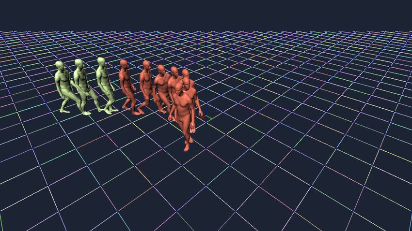
with the same latent space as the CVAE in DLow. ‘MOJO-         motion prediction sensitive to slight changes of the input.
proj’ is the model without recursive projection. Note that     Moreover, by comparing ‘VAE+DCT’ and ‘VAE+DCT+L’,
the suffixes can be concatenated; e.g. ‘MOJO-DCT-proj’ is      we can see that sampling from N (0, I) yields much worse
the model without the latent DCT space and without the re-     results. This indicates that sampling from the standard nor-
cursive projection scheme.                                     mal distribution, which treats all frequency bands equally,
                                                               cannot effectively exploit the advantage of the latent DCT
4.3. Evaluation of Stochastic Motion Prediction                space. Note that most information is in the low-frequency
4.3.1   Metrics                                                bands (see Appendix), and hence our proposed sampling
                                                               method utilizes the latent frequency space in a more rea-
Diversity. We use the same diversity measure as [57],          sonable way and produces better results.
which is the average pair-wise distance between all gener-
ated sequences.                                                4.4. Evaluation of Motion Realism
Prediction accuracy. As in [57], we use the average dis-       4.4.1   Metrics
tance error (ADE) and the final distance error (FDE) to
                                                               The motion prediction metrics cannot indicate whether a
measure the minimum distance between the generated mo-
                                                               motion is realistic or not. Here, we employ MOJO with re-
tion and the ground truth, w.r.t. frame-wise difference and
                                                               cursive projection to obtain 3D body meshes, and evaluate
the final frame difference, respectively. Additionally, we
                                                               the body deformation, foot skating, and perceptual quality.
use MMADE and MMFED to evaluate prediction accuracy
when the input sequence slightly changes; see Appendix.        Body deformation. Body shape can be described by the
                                                               pairwise distances between markers. As a body moves,
Motion Frequency. Similar to [22], we compute the fre-
                                                               there is natural variation in these distances. Large varia-
quency spectra entropy (FSE) to measure motion frequency
                                                               tions, however, indicate a deformed body that no longer cor-
in the Fourier domain, which is given by the averaged spec-
                                                               responds to any real person. We use variations in pairwise
tra entropy minus the ground truth. A higher value indicates
                                                               marker distances for the head, upper torso, and lower torso
the generated motions contain more motion detail. Note that
                                                               as a measure of how distorted the predicted body is. See
high frequency can also indicate noise, and hence this met-
                                                               Appendix for the metric details.
ric is jointly considered with the prediction accuracy.
                                                               Foot skating ratio. Foot skating is measured based on the
                                                               two markers on the lef and right foot calcaneus (‘LHEE’
4.3.2   Results                                                and ‘RHEE’ in CMU [1]). We consider foot skating to
We generate 50 different future sequences based on each        have occurred, when both foot markers are close enough to
input sequence, as in [57]. Here we focus only on evalu-       the ground (within 5cm) and simultaneously exceed a speed
ating performance on motion prediction, and hence do not       limit (5mm between two consecutive frames or 75mm/s).
incorporate the body re-projection scheme. The results are     We report the averaged ratio of frames with foot skating.
shown in Tab. 1, in which we employ DLow on the 20%            Perceptual score. We render the generated body meshes as
(i.e. the first 9) lowest frequency bands in ‘MOJO-proj’.      well as the ground truth, and perform a perceptual study on
We find that DCT consistently leads to better performance.     Amazon Mechanical Turk. Subjects see a motion sequence
Noticeably, higher motion frequency indicates that the gen-    and the statement “The human motion is natural and real-
erated motions contain more details, and hence are more        istic.” They evaluate this on a six-point Likert scale from
realistic.                                                     ‘strongly disagree‘ (1) to ‘strongly agree’ (6). Each individ-
    To further investigate the benefits of our latent DCT      ual video is rated by three subjects. We report mean values
space, we add the latent DCT space into the DLow CVAE          and standard deviations for each method and each dataset.
model [57] and train it with the robust KLD term. For sam-
pling, we apply a set of DLow models {Qw } on the lowest       4.4.2   Results
L bands, as in Sec. 3.3. We denote this modified model as
‘VAE+DCT+L’. Absence of the suffix ‘+L’ indicates sam-         We randomly choose 60 different sequences from ACCAD
pling from N (0, I) in all frequency bands.                    and BMLhandball, respectively. Based on each sequence,
    A comparison with existing methods is shown in Tab. 2.     we generate 15 future sequences. Figure 5 shows some gen-
Overall, our latent DCT space effectively improves on the      erated 3D body motions. The motions generated by MOJO
state-of-the-art. The diversity is improved by a large mar-    contain finer-grained body movements.
gin, while the prediction accuracies are comparable to the     Body deformation. The results are shown in Tab. 3. With
baseline. The performance w.r.t. MMADE and MMFDE is            the recursive projection scheme, the body shape is pre-
slightly inferior. A probable reason is VAE+DCT uses high-     served by construction and is close to the ground truth.
frequency components to generate motions, which makes          Without the projection scheme, the shape of body parts can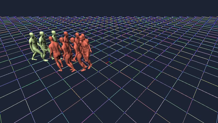
ACCAD [2]                                                              BMLHandball [21, 20]
  Method             Diversity↑         ADE↓       FDE↓       MMADE↓        MMFDE↓      FSE↑       Diversity↑     ADE↓        FDE↓      MMADE↓        MMFDE↓           FSE↑
  MOJO-DCT-proj      25.349             1.991      3.216      2.059         3.254       0.4        21.504         1.608       1.914     1.628         1.919            0.0
  MOJO-proj          28.886             1.993      3.141      2.042         3.202       1.2        23.660         1.528       1.848     1.550         1.847            0.4

Table 1: Comparison between generative models for predicting marker-based motions. The symbol ↓ (or ↑) denotes whether
results that are lower (or higher) are better, respectively. Best results of each model are in boldface. The FSE scores are on
the scale of 10−3 .

                                                           Human3.6M [25]                                                 HumanEva-I [48]
           Method                Diversity↑        ADE↓       FDE↓        MMADE↓      MMFDE↓       Diversity↑     ADE↓        FDE↓      MMADE↓         MMFDE↓
           Pose-Knows [50]              6.723      0.461      0.560        0.522       0.569            2.308     0.269       0.296       0.384           0.375
           MT-VAE [56]                  0.403      0.457      0.595        0.716       0.883            0.021     0.345       0.403       0.518           0.577
           HP-GAN [7]                   7.214      0.858      0.867        0.847       0.858            1.139     0.772       0.749       0.776           0.769
           Best-of-Many [8]             6.265      0.448      0.533        0.514       0.544            2.846     0.271       0.279       0.373           0.351
           GMVAE [14]                   6.769      0.461      0.555        0.524       0.566            2.443     0.305       0.345       0.408           0.410
           DeLiGAN [19]                 6.509      0.483      0.534        0.520       0.545            2.177     0.306       0.322       0.385           0.371
           DSF [58]                     9.330      0.493      0.592        0.550       0.599            4.538     0.273       0.290       0.364           0.340
           DLow [57]                   11.730      0.425      0.518        0.495       0.532            4.849     0.246       0.265       0.360           0.340
           VAE+DCT                      3.462      0.429      0.545        0.525       0.581            0.966     0.249       0.296       0.412           0.445
           VAE+DCT+5                   12.579      0.412      0.514        0.497       0.538            4.181     0.234       0.244       0.369           0.347
           VAE+DCT+20                  15.920      0.416      0.522        0.502       0.546            6.266     0.239       0.253       0.371           0.345

  Table 2: Comparison between a baseline with our latent DCT space and the state-of-the-art. Best results are in boldface.

                                                                                                                       ACCAD [2]                  BMLHandball [21, 20]
                                                                                               Method           foot skate     percep. score    foot skate    percep. score
                                                                                               MOJO-DCT           0.341         4.15±1.38         0.077           4.00±1.26
                                                                                               MOJO               0.278         4.07±1.31         0.066           4.17±1.23
                                                                                               Ground truth       0.067         4.82±1.08         0.002           4.83±1.05

                                                                                          Table 4: Comparison between methods w.r.t. foot skating
                                                                                          and the perceptual score, which is given by mean±std. Best
                                                                                          results are in boldface.

                                                                                          drift significantly from the true shape, indicated here by
                                                                                          high deformation numbers. MOJO is close to the ground
                                                                                          truth but exhibits less deformation suggesting that some nu-
                                                                                          ance is smoothed out by the VAE.
                                                                                          Foot skating and perceptual score. The results are pre-
                                                                                          sented in Tab. 4. The model with DCT produces fewer
Figure 5: Visualization of 3D body motions. Bodies in                                     foot skating artifacts, indicating that high-frequency com-
gray-green and red denote the input and the generated mo-                                 ponents in the DCT space can better model the foot move-
tion, respectively. The solid and dash image borders denote                               ments. In the perceptual study, MOJO performs slightly
the results from MOJO-DCT and MOJO, respectively.                                         worse than MOJO-DCT on ACCAD, but outperforms it on
                                                                                          BMLhandball. A probable reason is that most actions in
                              ACCAD [2]                    BMLHandball [21, 20]           ACCAD are coarse-grained, whereas most actions in BML-
 Method             Head       Up. T.      Low. T.     Head      Up. T.     Low. T.       handball are fine-grained. The advantage of modelling
 MOJO-DCT-proj      76.3       102.2        99.4       86.0      105.3       83.3
                                                                                          finer-grained motion of the DCT latent space is more easily
 MOJO-proj          70.3        80.7        76.7       68.3       77.7       63.2         perceived in BMLhandball.
 MOJO-DCT           1.32        34.0        6.97       1.32       43.1       6.97
 MOJO               1.30        32.7        6.76       1.40       44.3       7.64         4.5. Comparison between Body Representations
 Ground truth       2.17        36.4        9.78       2.52       59.1       12.5
                                                                                             The body in motion can be represented by locations of
Table 3: Deformations of body parts (head, Upper Torso,                                   joints, markers with different placements, and their com-
Lower Torso). Scores are in millimeter. High values indi-                                 binations. Here we perform a systematic comparison be-
cate distorted bodies.                                                                    tween them. For the joint-based representation, we use the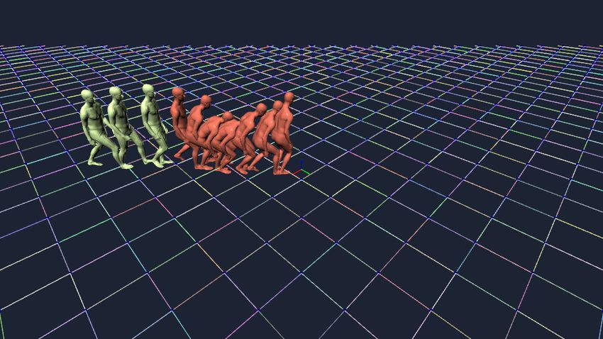
ACCAD [2]                                           BMLHandball [21, 20]
  Method             Diversity↑   ADE↓    FDE↓    MMADE↓   MMFDE↓   BDF↓    Diversity↑   ADE↓     FDE↓     MMADE↓       MMFDE↓   BDF↓
  joints w/o proj.   21.363       1.184   2.010   1.291    2.067    0.185   19.091       0.930    1.132    1.000        1.156    0.205
  joints             21.106       1.192   2.022   1.299    2.076    0       18.954       0.934    1.138    1.003        1.157    0
  CMU 41             20.676       1.214   1.919   1.306    2.080    0       16.806       0.949    1.139    1.001        1.172    0
  SSM2 67            24.373       1.124   1.699   1.227    1.838    0       18.778       0.924    1.099    0.975        1.149    0
  joints + CMU 41    20.988       1.187   1.841   1.308    1.967    0       13.982       0.943    1.190    0.990        1.194    0
  joints + SSM2 67   23.504       1.166   1.892   1.276    1.953    0       16.483       0.950    1.146    0.999        1.189    0

Table 5: Comparison between marker-based and joint-based representations. Evaluations are based on the joint locations.
BDF denotes the bone deformation w.r.t. meter. The best results are in boldface.

SMPL [33] joint locations from CMU and MPI HDM05 to
train a CVAE as in MOJO. A traditional pipeline is to first
predict all joints in the future, and then fit the body mesh.
Here we also test the performance when applying the re-
cursive body re-projection scheme based on joints. For fair
quantitative evaluation, the metrics are calculated based on
the joints of the fitted body meshes. We re-calculate the di-
versity, the prediction accuracy metrics, and the eight limb
bone deformation (BDF) (according to Eq. (6) in Appendix)
w.r.t. the joint locations.
    We randomly choose 60 sequences from each test set and
generate 50 future motions based on each sequence. Re-
sults are presented in Tab. 5. The first two rows show that
the motion naturalness is improved by the recursive pro-             Figure 6: Fitting a character to predicted joints. The top
jection, which eliminates the bone deformation. Although             row and the bottom row show the predicted skeletons and
the result without projection is slightly better on other mea-       the fitted bodies, respectively. From left to right: The first
sures, the projection scheme completely removes bone de-             predicted frame, the middle frame, and the last frame.
formation and does not produce false poses as in Fig. 6.
Additionally, using more markers (SSM2 placement with                tion, MOJO uses a recursive projection scheme at test time.
67 markers) significantly improves performance across the            By fitting a SMPL-X body to the predicted markers at each
board. This shows that the marker distribution is impor-             frame, the 3D bodies stay valid over time and motion real-
tant for motion prediction and that more markers is better.          ism is improved. Compared to a traditional pipeline based
While MOJO works with markers, joints, or the combina-               on joints, MOJO thoroughly eliminates implausible body
tion of both, the combination of joints and markers does not         deformations and produces realistic 3D body movements.
produce better performance. Note that the joints are never              Nevertheless, MOJO has some limitations to improve in
directly observed, but rather are inferred from the markers          the future. For example, the recursive projection scheme
by commercial mocap systems. Hence, we argue that the                slows down the inference process. Also, the motion realism
joints do not add independent information.                           is still not comparable with the ground truth (see Tab. 4),
    Figure 6 shows the risk of the traditional joint-based           indicating room to improve. Moreover, we will explore the
pipeline. While the skeletons may look fine to the eye, in           performance of MOJO on other marker settings, or even real
the last frame the character cannot be fit to the joints due to      markers from mocap data.
unrealistic bone lengths.
                                                                     Acknowledgement: We thank Nima Ghorbani for the advice on
5. Conclusion                                                        the body marker setting and the AMASS dataset. We thank Ying-
                                                                     hao Huang, Cornelia Köhler, Victoria Fernández Abrevaya, and
   In this paper, we propose MOJO, a new method to pre-              Qianli Ma for proofreading. We thank Xinchen Yan and Ye Yuan
dict diverse plausible motions of 3D bodies. Instead of us-          for discussions on baseline methods. We thank Shaofei Wang and
ing joints to represent the body, MOJO uses a sparse set             Siwei Zhang for their help with the user study and the presentation,
of markers on the body surface, which better constrain 3D            respectively.
body shape and pose recovery. In contrast to most existing           Disclaimer: MJB has received research gift funds from Adobe,
methods that encode a motion into a single feature vector,           Intel, Nvidia, Facebook, and Amazon. While MJB is a part-time
we represent motion with latent frequencies, which can de-           employee of Amazon, his research was performed solely at, and
scribe fine-grained body movements and improve motion                funded solely by, Max Planck. MJB has financial interests in Ama-
prediction consistently. To produce valid 3D bodies in mo-           zon Datagen Technologies, and Meshcapade GmbH.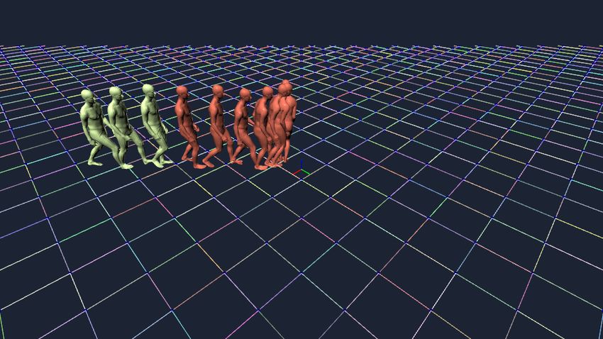
References                                                          [14] Nat Dilokthanakul, Pedro AM Mediano, Marta Garnelo,
                                                                         Matthew CH Lee, Hugh Salimbeni, Kai Arulkumaran, and
 [1] CMU graphics lab. CMU graphics lab motion capture                   Murray Shanahan. Deep unsupervised clustering with
     database. http://mocap.cs.cmu.edu/, 2000. 4, 5,                     gaussian mixture variational autoencoders. arXiv preprint
     6, 1, 3                                                             arXiv:1611.02648, 2016. 3, 7
 [2] ACCAD MoCap System and Data. https://accad.                    [15] Partha Ghosh, Jie Song, Emre Aksan, and Otmar Hilliges.
     osu . edu / research / motion - lab / systemdata,                   Learning human motion models for long-term predictions.
     2018. 5, 7, 8                                                       In International Conference on 3D Vision, pages 458–466.
 [3] Nasir Ahmed, T. Natarajan, and Kamisetty R. Rao. Dis-               IEEE, 2017. 3
     crete cosine transform. IEEE transactions on Computers,        [16] Anand Gopalakrishnan, Ankur Mali, Dan Kifer, Lee Giles,
     100(1):90–93, 1974. 2, 4                                            and Alexander G Ororbia. A neural temporal model for hu-
 [4] Ijaz Akhter, Tomas Simon, Sohaib Khan, Iain Matthews, and           man motion prediction. In IEEE Conference on Computer
     Yaser Sheikh. Bilinear spatiotemporal basis models. ACM             Vision and Pattern Recognition, pages 12116–12125, 2019.
     Transactions on Graphics, 31(2):1–12, 2012. 3                       3
 [5] Emre Aksan, Peng Cao, Manuel Kaufmann, and Otmar               [17] Liang-Yan Gui, Yu-Xiong Wang, Xiaodan Liang, and
     Hilliges.    Attention, please: A spatio-temporal trans-            José MF Moura. Adversarial geometry-aware human mo-
     former for 3D human motion prediction. arXiv preprint               tion prediction. In European Conference on Computer Vi-
     arXiv:2004.08692, 2020. 3                                           sion, pages 786–803, 2018. 3, 5
 [6] Emre Aksan, Manuel Kaufmann, and Otmar Hilliges. Struc-        [18] Liang-Yan Gui, Yu-Xiong Wang, Deva Ramanan, and
     tured prediction helps 3D human motion modelling. In IEEE           José MF Moura. Few-shot human motion prediction via
     Conference on Computer Vision and Pattern Recognition,              meta-learning. In European Conference on Computer Vision,
     pages 7144–7153, 2019. 3                                            pages 432–450, 2018. 3
 [7] Emad Barsoum, John Kender, and Zicheng Liu. HP-GAN:            [19] Swaminathan Gurumurthy, Ravi Kiran Sarvadevabhatla, and
     Probabilistic 3D human motion prediction via GAN. In IEEE           R Venkatesh Babu. DeLiGAN: Generative adversarial net-
     Conf. Comput. Vis. Pattern Recog. Worksh., pages 1418–              works for diverse and limited data. In IEEE Conference on
     1427, 2018. 3, 7                                                    Computer Vision and Pattern Recognition, pages 166–174,
                                                                         2017. 3, 7
 [8] Apratim Bhattacharyya, Bernt Schiele, and Mario Fritz. Ac-
                                                                    [20] Fabian Helm, Rouwen Cañal-Bruland, David L Mann, Niko-
     curate and diverse sampling of sequences based on a “best of
                                                                         laus F Troje, and Jörn Munzert. Integrating situational proba-
     many” sample objective. In IEEE Conference on Computer
                                                                         bility and kinematic information when anticipating disguised
     Vision and Pattern Recognition, pages 8485–8493, 2018. 3,
                                                                         movements. Psychology of Sport and Exercise, 46:101607,
     7
                                                                         2020. 5, 7, 8
 [9] Federica Bogo, Angjoo Kanazawa, Christoph Lassner, Peter       [21] Fabian Helm, Nikolaus F Troje, and Jörn Munzert. Mo-
     Gehler, Javier Romero, and Michael J. Black. Keep it SMPL:          tion database of disguised and non-disguised team handball
     Automatic estimation of 3D human pose and shape from a              penalty throws by novice and expert performers. Data in
     single image. In European Conference on Computer Vision,            brief, 15:981–986, 2017. 5, 7, 8
     Oct. 2016. 4
                                                                    [22] Alejandro Hernandez, Jurgen Gall, and Francesc Moreno-
[10] Yujun Cai, Lin Huang, Yiwei Wang, Tat-Jen Cham, Jianfei             Noguer. Human motion prediction via spatio-temporal in-
     Cai, Junsong Yuan, Jun Liu, Xu Yang, Yiheng Zhu, Xiao-              painting. In IEEE Conference on Computer Vision and Pat-
     hui Shen, et al. Learning progressive joint propagation for         tern Recognition, pages 7134–7143, 2019. 3, 5, 6
     human motion prediction. In European Conference on Com-        [23] Daniel Holden, Ikhsanul Habibie, Ikuo Kusajima, and Taku
     puter Vision, 2020. 3                                               Komura. Fast neural style transfer for motion data. IEEE
[11] Pierre Charbonnier, Laure Blanc-Feraud, Gilles Aubert, and          computer graphics and applications, 37(4):42–49, 2017. 3
     Michel Barlaud. Two deterministic half-quadratic regular-      [24] Yinghao Huang, Federica Bogo, Christoph Lassner, Angjoo
     ization algorithms for computed imaging. In Proceedings             Kanazawa, Peter V Gehler, Javier Romero, Ijaz Akhter, and
     of the International Conference on Image Processing, pages          Michael J Black. Towards accurate marker-less human shape
     168–172, 1994. 4                                                    and pose estimation over time. In International Conference
[12] Kyunghyun Cho, Bart van Merriënboer, Caglar Gulcehre,              on 3D Vision, pages 421–430. IEEE, 2017. 3
     Dzmitry Bahdanau, Fethi Bougares, Holger Schwenk, and          [25] Catalin Ionescu, Dragos Papava, Vlad Olaru, and Cristian
     Yoshua Bengio. Learning phrase representations using RNN            Sminchisescu. Human3.6M: Large scale datasets and pre-
     encoder–decoder for statistical machine translation. In Pro-        dictive methods for 3D human sensing in natural environ-
     ceedings of the Conference on Empirical Methods in Natural          ments. IEEE Transactions on Pattern Analysis and Machine
     Language Processing, pages 1724–1734, Doha, Qatar, Oct.             intelligence, 36(7):1325–1339, 2014. 2, 5, 7
     2014. 4                                                        [26] Diederik P Kingma and Max Welling. Auto-encoding varia-
[13] Qiongjie Cui, Huaijiang Sun, and Fei Yang. Learning dy-             tional Bayes. In International Conference on Learning Rep-
     namic relationships for 3D human motion prediction. In              resentions, 2014. 4
     IEEE Conference on Computer Vision and Pattern Recog-          [27] Muhammed Kocabas, Nikos Athanasiou, and Michael J.
     nition, pages 6519–6527, 2020. 3                                    Black. VIBE: Video inference for human body pose and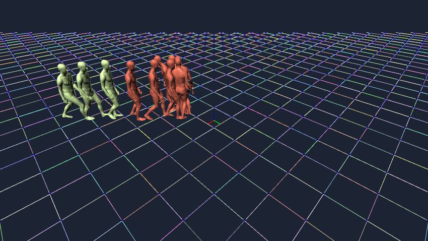
shape estimation. In IEEE Conference on Computer Vision                tion Processing Systems 32, pages 8024–8035. Curran Asso-
       and Pattern Recognition, pages 5252–5262, 2020. 5                      ciates, Inc., 2019. 2
[28]   Chen Li, Zhen Zhang, Wee Sun Lee, and Gim Hee Lee. Con-         [41]   Georgios Pavlakos, Vasileios Choutas, Nima Ghorbani,
       volutional sequence to sequence model for human dynamics.              Timo Bolkart, Ahmed A. A. Osman, Dimitrios Tzionas, and
       In IEEE Conference on Computer Vision and Pattern Recog-               Michael J. Black. Expressive body capture: 3D hands, face,
       nition, pages 5226–5234, 2018. 3                                       and body from a single image. In IEEE Conference on Com-
[29]   Maosen Li, Siheng Chen, Yangheng Zhao, Ya Zhang, Yan-                  puter Vision and Pattern Recognition, pages 10975–10985,
       feng Wang, and Qi Tian. Dynamic multiscale graph neural                June 2019. 2, 3, 4
       networks for 3D skeleton based human motion prediction. In      [42]   Dario Pavllo, Christoph Feichtenhofer, Michael Auli, and
       IEEE Conference on Computer Vision and Pattern Recogni-                David Grangier. Modeling human motion with quaternion-
       tion, pages 214–223, 2020. 3                                           based neural networks. International Journal of Computer
[30]   Hung Yu Ling, Fabio Zinno, George Cheng, and Michiel Van               Vision, pages 1–18, 2019. 3
       De Panne. Character controllers using motion VAEs. ACM          [43]   Dario Pavllo, David Grangier, and Michael Auli. Quaternet:
       Transactions on Graphics, 39(4):40–1, 2020. 3                          A quaternion-based recurrent model for human motion. In
[31]   Hongyi Liu and Lihui Wang. Human motion prediction for                 British Machine Vision Conference, 2018. 3, 4
       human-robot collaboration. Journal of Manufacturing Sys-        [44]   K. Pullen and C. Bregler. Animating by multi-level sam-
       tems, 44:287–294, 2017. 2                                              pling. In Proceedings Computer Animation 2000, pages 36–
                                                                              42, 2000. 3
[32]   Matthew Loper, Naureen Mahmood, and Michael J Black.
       Mosh: Motion and shape capture from sparse markers. ACM         [45]   K Ramamohan Rao and Ping Yip. Discrete cosine trans-
       Transactions on Graphics, 33(6):1–13, 2014. 2, 4, 5                    form: algorithms, advantages, applications. Academic
                                                                              press, 2014. 2, 4
[33]   Matthew Loper, Naureen Mahmood, Javier Romero, Ger-
                                                                       [46]   Javier Romero, Dimitrios Tzionas, and Michael J. Black.
       ard Pons-Moll, and Michael J. Black. SMPL: A skinned
                                                                              Embodied Hands: Modeling and capturing hands and bod-
       multi-person linear model. ACM Transactions on Graphics,
                                                                              ies together. ACM Transactions on Graphics, (Proc. SIG-
       34(6):248:1–248:16, Oct. 2015. 2, 3, 8
                                                                              GRAPH Asia), 36(6), Nov. 2017. 3
[34]   Naureen Mahmood, Nima Ghorbani, Nikolaus F. Troje, Ger-
                                                                       [47]   Andrey Rudenko, Luigi Palmieri, Michael Herman, Kris M
       ard Pons-Moll, and Michael J. Black. AMASS: Archive of
                                                                              Kitani, Dariu M Gavrila, and Kai O Arras. Human motion
       motion capture as surface shapes. In International Confer-
                                                                              trajectory prediction: A survey. The International Journal of
       ence on Computer Vision, pages 5442–5451, Oct. 2019. 2,
                                                                              Robotics Research, 39(8):895–935, 2020. 2
       4, 5, 1
                                                                       [48]   Leonid Sigal, Alexandru O Balan, and Michael J Black. Hu-
[35]   Wei Mao, Miaomiao Liu, Mathieu Salzmann, and Hongdong                  manEva: Synchronized video and motion capture dataset and
       Li. Learning trajectory dependencies for human motion pre-             baseline algorithm for evaluation of articulated human mo-
       diction. In International Conference on Computer Vision,               tion. International Journal of Computer Vision, 87(1-2):4,
       pages 9489–9497, 2019. 3                                               2010. 2, 5, 7
[36]   Julieta Martinez, Michael J Black, and Javier Romero. On        [49]   Yongyi Tang, Lin Ma, Wei Liu, and Wei-Shi Zheng. Long-
       human motion prediction using recurrent neural networks. In            term human motion prediction by modeling motion context
       IEEE Conference on Computer Vision and Pattern Recogni-                and enhancing motion dynamic. In International Joint Con-
       tion, pages 2891–2900, 2017. 3, 4                                      ference on Artificial Intelligence, page 935–941, 2018. 3
[37]   Meinard Müller, Tido Röder, Michael Clausen, Bernhard         [50]   Jacob Walker, Kenneth Marino, Abhinav Gupta, and Martial
       Eberhardt, Björn Krüger, and Andreas Weber. Documen-                 Hebert. The pose knows: Video forecasting by generating
       tation mocap database HDM05. 2007. 5                                   pose futures. In International Conference on Computer Vi-
[38]   Dirk Ormoneit, Hedvig Sidenbladh, Michael Black, and                   sion, pages 3332–3341, 2017. 3, 7
       Trevor Hastie. Learning and tracking cyclic human mo-           [51]   Mao Wei, Liu Miaomiao, and Salzemann Mathieu. History
       tion. Advances in Neural Information Processing Systems,               repeats itself: Human motion prediction via motion atten-
       13:894–900, 2000. 3                                                    tion. In European Conference on Computer Vision, 2020.
[39]   Ahmed A. A. Osman, Timo Bolkart, and Michael J. Black.                 3
       STAR: Sparse trained articulated human body regressor. In       [52]   Xinshuo Weng, Jianren Wang, Sergey Levine, Kris Kitani,
       European Conference on Computer Vision, volume LNCS                    and Nick Rhinehart. 4D Forecasting: Sequantial Forecasting
       12355, pages 598–613, Aug. 2020. 3, 1                                  of 100,000 Points. Euro. Conf. Comput. Vis. Worksh., 2020.
[40]   Adam Paszke, Sam Gross, Francisco Massa, Adam Lerer,                   3
       James Bradbury, Gregory Chanan, Trevor Killeen, Zeming          [53]   Xinshuo Weng, Jianren Wang, Sergey Levine, Kris Kitani,
       Lin, Natalia Gimelshein, Luca Antiga, Alban Desmaison,                 and Nick Rhinehart. Inverting the Pose Forecasting Pipeline
       Andreas Kopf, Edward Yang, Zachary DeVito, Martin Rai-                 with SPF2: Sequential Pointcloud Forecasting for Sequential
       son, Alykhan Tejani, Sasank Chilamkurthy, Benoit Steiner,              Pose Forecasting. CoRL, 2020. 3
       Lu Fang, Junjie Bai, and Soumith Chintala. Pytorch: An im-      [54]   Erwin Wu and Hideki Koike. Futurepong: Real-time table
       perative style, high-performance deep learning library. In H.          tennis trajectory forecasting using pose prediction network.
       Wallach, H. Larochelle, A. Beygelzimer, F. d'Alché-Buc, E.            In Extended Abstracts of the 2020 CHI Conference on Hu-
       Fox, and R. Garnett, editors, Advances in Neural Informa-              man Factors in Computing Systems, pages 1–8, 2020. 2
[55] Hongyi Xu, Eduard Gabriel Bazavan, Andrei Zanfir,
William T Freeman, Rahul Sukthankar, and Cristian Smin-
chisescu. GHUM & GHUML: Generative 3D human shape
and articulated pose models. In IEEE Conference on Com-
puter Vision and Pattern Recognition, pages 6184–6193,
2020. 3, 1
[56] Xinchen Yan, Akash Rastogi, Ruben Villegas, Kalyan
Sunkavalli, Eli Shechtman, Sunil Hadap, Ersin Yumer, and
Honglak Lee. MT-VAE: Learning motion transformations to
generate multimodal human dynamics. In European Confer-
ence on Computer Vision, pages 265–281, 2018. 3, 7
[57] Ye Yuan and Kris Kitani. DLow: Diversifying latent flows
for diverse human motion prediction. European Conference
on Computer Vision, 2020. 2, 3, 4, 5, 6, 7, 1
[58] Ye Yuan and Kris M. Kitani. Diverse trajectory forecasting
with determinantal point processes. In International Confer-
ence on Learning Representions, 2020. 7
[59] M Ersin Yumer and Niloy J Mitra. Spectral style transfer for
human motion between independent actions. ACM Transac-
tions on Graphics, 35(4):1–8, 2016. 3
[60] Jason Y Zhang, Panna Felsen, Angjoo Kanazawa, and Jiten-
dra Malik. Predicting 3D human dynamics from video. In
International Conference on Computer Vision, pages 7114–
7123, 2019. 2
[61] Yan Zhang, Michael J Black, and Siyu Tang. Perpetual mo-
tion: Generating unbounded human motion. arXiv preprint
arXiv:2007.13886, 2020. 2, 3, 4
[62] Yi Zhou, Connelly Barnes, Jingwan Lu, Jimei Yang, and Hao
Li. On the continuity of rotation representations in neural
networks. In IEEE Conference on Computer Vision and Pat-
tern Recognition, pages 5745–5753, 2019. 3
[63] Yi Zhou, Zimo Li, Shuangjiu Xiao, Chong He, Zeng Huang,
and Hao Li. Auto-conditioned recurrent networks for ex-
tended complex human motion synthesis. In International
Conference on Learning Representions, 2018. 3We are More than Our Joints: Predicting how 3D Bodies Move
**Appendix**
MOJO is implemented using SMPL-X but any other parametric 3D body model could be used, e.g. [39, 55]. To do so,
one only needs to implement the recursive fitting of 3D pose to observed markers. This is a straightforward optimization
problem. In this paper, we use SMPL-X to demonstrate our MOJO idea, because we can exploit the large-scale AMASS
dataset to train/test our networks. Moreover, SMPL-X is rigged with a skeleton like other body models in computer graphics,
so it is completely compatible with standard skeletal techniques.
A. More Method Details
Marker placements in our work. In our experiments, we use two kinds of marker placements. The first (default) one is
the CMU [1] setting with 41 markers. The second one is the SSM2 [34] setting with 67 markers. These marker settings are
illustrated in Fig. S1.
CMU placement, 41 markers
SSM2 placement, 67 markers
Figure S1: Illustration of our marker settings. The markers are denoted by 3D spheres attached to the SMPL-X body surface.
From left to right: the front view, the back view and the top view.
Network architectures. We have demonstrated the CVAE architecture of MOJO in Sec. 3, and compare it with several
baselines and variants in Sec. 4. The architectures of the used motion generators are illustrated in Fig. S2. Compared to the
CVAE of MOJO, VAE+DCT has no residual connections at the output, and the velocity reconstruction loss is replaced by a
loss to minimize |xM − y0 |2 [57]. MOJO-DCT-proj encodes the motion Y into a single feature vector, rather than a set of
frequency components.condition module encoder decoder
GRU fc
MOJO-proj GRU c fc 1
c GRU fc +
I
D
D
GRU c C fc 1
c GRU fc +
C
T
T
GRU c fc 1
c GRU fc +
…
…
…
…
…
GRU fc
GRU c fc c GRU fc +
MOJO-DCT-proj
1
Y
c GRU fc +
c GRU fc +
…
GRU fc
GRU c fc 1
c GRU fc
I
VAE+DCT D
D
GRU c C fc 1
c GRU fc
C
T
T
GRU c fc 1
c GRU fc
…
…
…
…
…
Figure S2: From top to bottom: (1) The CVAE architecture of MOJO. (2) The CVAE architecture of MOJO-DCT, which is
used in Tables 1 3 4. (3) The architecture of VAE+DCT, which is evaluated in Tab. 2. Note that we only illustrate the motion
generators here. The recursive projection scheme can be added during the testing time.
B. More Experimental Details
Implementation. We use PyTorch v1.6.0 [40] in our experiments. In the training loss Eq. (1), we empirically set α = 3
in all cases. We find a larger value causes over-smooth and loses motion details, whereas a smaller value can cause jitters.
For the models with the latent DCT space, the robust KLD term with the loss weight 1 is employed. For models without the
latent DCT space, we use a standard KLD term, and set its weight to 0.1. The weights of the KLD terms are not annealed
during training. In the fitting loss Eq. (2), we empirically set {λ1 , λ2 } = {0.0005, 0.01}. Smaller values can degrade the
pose realism with e.g. twisted torsos, and larger values reduce the pose variations in motion. Our code is publicly released,
which delivers more details.
The model ‘MOJO-DCT-proj’ has a latent dimension of 128. However, ‘MOJO-proj’ suffers from overfitting with the
same latent dimension, and hence we set its latent dimension to 16. We use these dimensions in all experiments.
AMASS sequence canonicalization. To unify the sequence length and world coordinates, we canonicalize AMASS as
follows: First, we trim the original sequences into 480-frame (4-second) subsequences, and downsample them from 120fps
to 15fps. The condition sequence X contains 15 frames (1s) and the future sequence Y contains 45 frames (3s). Second, weunify the world coordinates as in [61]. For each subsequence, we reset the world coordinate to the SMPL-X [41] body mesh
in the first frame: The horizontal X-axis points in the direction from the left hip to the right hip, the Z-axis is the negative
direction of gravity, and the Y-axis is pointing forward. The origin is set to to the body’s global translation.
More discussions on MMADE and MMFDE. As in [57], we use MMADE and MMFED to evaluate prediction accuracy
when the input sequence slightly changes. They are regarded as multi-modal version of ADE and FDE, respectively. Let’s
only demonstrate MMADE with more details here, since the same principle applies to MMFDE.
The ADE can be calculated by
1
eADE (Y) = min |Y − Ygt |2 , (3)
T Y ∈Y
in which Y is a predicted motion, Y is the set of all predicted motions, and Ygt is the ground truth future motion. In this
case, the MMADE can be calculate as
1
eMMADE (Y) = EY ∗ ∈YS min |Y − Y ∗ |2 (4)
T Y ∈Y
with
Ys = {Y ∗ ∈ Ygt | d(X ∗ , Xgt ) < η}, (5)
with Ygt is the set of all ground truth future motion, X denotes the corresponding motion in the past, d(·) is a difference
measure, and η is a pre-defined threshold. In the work of DLow [57], the difference measure d(·) is based on the L2 difference
between the last frames of the two motion sequences from the past.
Body deformation metric. We measure the markers on the head, the upper torso and the lower torso, respectively. Specif-
ically, according to CMU [1], we measure (‘LFHD’, ‘RFHD’, ‘RBHD’, ‘LBHD’) for the head, (‘RSHO’, ‘LSHO’, ‘CLAV’,
‘C7’) for the upper torso, and (‘RFWT’, ‘LFWT’, ‘LBWT’, ‘RBWT’) for the lower torso. For each rigid body part P , the
deformation score is the variations of marker pair-wise distances, and is calculated by
X
sd (P ) = EY σt (|vit − vjt |2 ) , (6)
(i,j)∈P
in which vit denotes the location of the marker i at time t, σt denotes the standard deviation along the time dimension, and
EY [·] denotes averaging the scores of different predicted sequences.
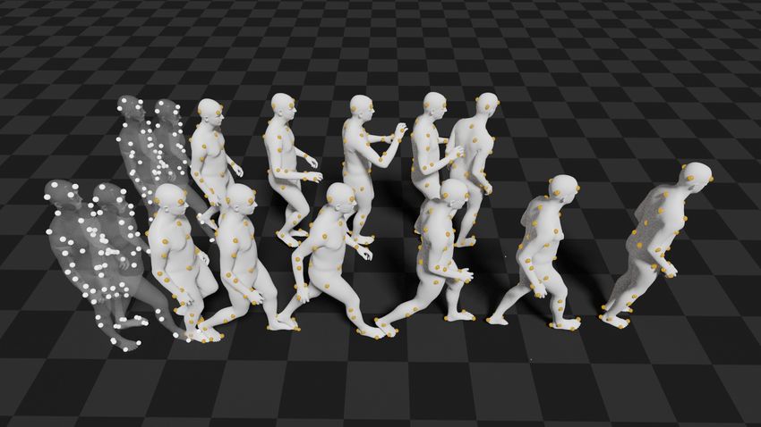
User study interface. Our user study is performed via AMT. The interface is illustrated in Fig. S3. We set a six-point
Likert scale for evaluation. Each video is evaluated by three subjects.
Performance of the original VAE setting in DLow. Noticeably, the DLow CVAE with the original setting cannot directly
work on body markers, although it works well with joint locations. Following the evaluation in Tab. 1, the original VAE
setting in DLow gives (diversity=81.10, ADE=2.79, FDE=4.71, MMADE=2.81, MMFDE=4.71, FSE=0.0031). The diversity
is much higher, but the accuracy is considerably worse. Fig. S4 shows that its predicted markers are not valid.
Influence of the given frames. Based on the CMU markers, we train another two MOJO versions with different in-
put/output sequence lengths. The results are in Tab. S1. As the predicted sequence becomes shorter and the input sequence
becomes longer, we can see that the accuracy increases but the diversity decreases consistently, indicating that MOJO be-
comes more confident and deterministic. Such behavior is similar to other state-of-the-art methods like DLow. Furthermore,
to predict even longer motion sequences, one could use a sliding window, and recursively input the predicted sequence to the
pre-trained MOJO model to generate new sequences.You can also read