Who pays for a Value Added Tax Hike at an International Border? Evidence from Mexico
←
→
Page content transcription
If your browser does not render page correctly, please read the page content below
Who pays for a Value Added Tax Hike at an
           International Border? Evidence from Mexico∗
                    Emmanuel Chávez†                  Cristobal Domı́nguez‡

                                         October 18, 2021

                                               Abstract

       This research studies the effects of a value added tax (VAT) reform at Mexico’s interna-
       tional frontiers. The reform raised the VAT rate from 11 to 16 percent at localities close
       to the international borders. We use the traditional “static” difference-in-differences
       methodology as well as dynamic difference-in-differences. The treatment group is com-
       posed of municipalities in the area where the VAT increased, and the control group is
       composed of municipalities close to the treatment group. We find that the VAT hike
       had a positive effect on prices of around half the size of the full pass-through conter-
       factual. In addition, the reform had a negative effect on workers’ wages and no effect
       on employment. The negative effect on workers’ real incomes is not smoothed out with
       credits. We find evidence of a negative effect on consumption at Mexico’s northern
       border due to the reform. However, we find no evidence of an increase in shopping at
       the United States side of the border.

       Keywords: Value Added Tax, Tax Incidence, Cross-border Shopping.

       JEL Codes: H22, H24, H73

   ∗
      We are grateful to Antoine Bozio, Jimmy Lopez, Loriane Py and Daniel Miranda for their valuable and
detailed comments throughout this research. In addition, are grateful from helpful comments from Raymundo
Campos-Vázquez, David Margolis, Ariell Reshef, Oliver Vanden Enyde, Anne-Célia Disdier, Alberto Aguilar,
Carmel Connell and seminar participants at Paris School of Economics and Comisión Nacional Bancaria
y de Valores (CNBV). Furthermore, we thank Consejo nacional de Ciencia y Tecnologı́a (CONACYT) for
financial funding through its doctoral scholarships. Administrative data collected by CNBV was manipulated
by Cristobal Domı́nguez following CNBV’s guidelines to protect data security. The comments, opinions and
conclusions in this paper are of our own and do not reflect those of CONACYT or CNBV.
    †
      Corresponding author. PhD candidate at Paris School of Economics.
    ‡
      Researcher at Comisión Nacional Bancaria y de Valores.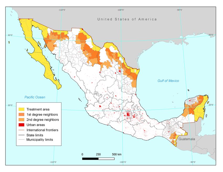
1       Introduction

Who pays for taxes is a longstanding question in economic thought. There is a long tradi-
tion in research among public economists that aims to determine how the burden of a tax
is allocated among consumers, workers or capital.1 Consumption taxes are not exempt of
this incidence analysis. Traditionally, research has focused on the effects of consumption
taxes on consumers through the effects on prices (Creedy, 2002; Kaplanoglou, 2004; Warren
et al., 2005; Barret and Wall, 2006; Garfinkel et al., 2006; Decoster et al., 2007; Warren,
2008; Gaarder, 2018; Mariscal and Werner, 2018). But recent studies on the incidence of
consumption taxes find that they have direct impacts on outcomes that go beyond prices,
such as profits (Kosonen, 2015; Harju et al., 2018; Benzarti and Carloni, 2019; Benzarti
et al., 2020). Our research builds on this strand of literature by analyzing an unusual value
added tax (VAT) reform. The reform took place in Mexico. It increased the VAT rate only
at the international frontiers. Specifically, the reform increased the VAT rate in localities
close to the borders from 11 to 16 percent in order to standardize the rate with that of the
rest of the country. The examination of this natural experiment allows to fill a gap in the
VAT incidence literature: what are the effects of raising the VAT if firms are exposed to
competition from a jurisdiction that does not raise consumption taxes?

    We obtain relevant findings that increase the current state of knowledge on the incidence
of the value added tax. First, we find the VAT hike led prices to increase. However, the size
of the effect is of around half the size of the full pass-through counterfactual. Prices do not
catch-up with the full pass-through in the whole period we analyze. This is relevant, as many
papers in this literaute find that VAT hikes are (at least) fully passed to consumers.2 We
argue that the relatively small pass-through we find is due to the context that we analyze:
if a country raises the VAT rate in the whole territory, consumers have limited options to
move and find better prices in case the hike is fully passed to the consumer. However, if the
    1
     A review of theoretical studies can be found in Kotlikoff and Summers (1987) and in Fullerton and
Metcalf (2002)
   2
     Benzarti and Carloni (2019) carry out an extensive analysis on the price incidence of VAT reforms in
Europe. They find that VAT hikes are fully passed to consumers in three months following the reform.

                                                   1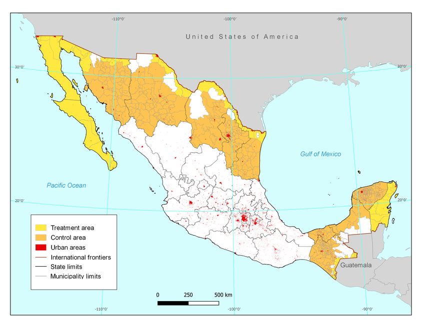
VAT rate is raised at international borders, consumers have more opportunities to search for
better prices. So, as firms are exposed to heavy competition at the border, they may refuse
to fully pass the tax hike on consumers, since they could lose demand to foreign sellers.3
Indeed, this was one of the main concerns of social demonstrations and political lobbying
against the VAT reform of 2013.4

    Our second key finding complements the first. We find that the VAT reform had a nega-
tive effect on wages of around 2.0 percent; with no effect on the level of employment.5 To our
knowledge, the causal effect of the VAT on wages is documented in just one previous study.
Benzarti and Carloni (2019) show that workers’ wages can benefit from VAT cuts. We are
the first to show that the opposite is also true: workers’ wages can be negatively affected by
VAT hikes. Our findings on prices and wages are consistent with VAT incidence literature
regarding how firms use VAT reforms to preserve or increase their profits.6 In the context we
study, firms are unable to pass the VAT hike fully on prices due to competition at the other
side of the border. However, they can adjust on labor costs by taking a (counterfactual) bite
on workers’ wages.

    Our third key finding is novel in the VAT incidence literature. We find that the VAT hike
had a negative effect on the number of payroll credits granted to workers. These are credits
whose payments are directly discounted from workers’ payrolls. To our knowledge, this is
the first paper that finds a causal effect of the VAT on the credit market. This extends the
   3
      Research by Carbonnier (2007, 2008) supports the view that the effect of VAT reforms on prices depends
on the context. He finds that prices change differently according to the degree of competition in the market
in response to changes in the VAT rate.
    4
      We describe the context of the reform with more detail in Section 2.
    5
      As point of reference, the average annual growth of the nominal minimum wage in Mexico in the 10
years previous to the reform was 4.5 percent. So, if typical wage growth in Mexico is taken into account, the
size of the effect that we find is considerable.
    6
      Kosonen (2015) finds that about half of a VAT cut in Finland was passed to prices, enabling firms to
increase their profits after the tax cut. Benzarti and Carloni (2019) study a VAT cut in France and show
that most of the gains from the tax cut were pocketed by employers, with a small part going to consumers
and employees. Benzarti et al. (2020) analyze VAT increases in several European countries. They find
that firms increase prices at a rate that exceeds that of the full pass-through, increasing their profits as a
consequence. This finding is supported by research in Hungary by Ván and Oláh (2018). Harju et al. (2018)
study restaurant VAT cuts in Finland and Sweden and find no reduction of prices in independent restaurants
due to these cuts.

                                                      2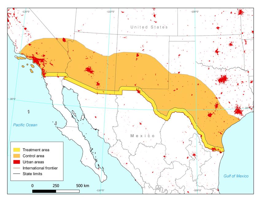
existing evidence on the set of outcomes that can be affected by the VAT. This finding is in
line with the literature that finds that income shocks are not smoothed-out, which contra-
dicts a key prediction of the standard consumption smoothing theory.7

    In addition, we study the cross-border shopping dimension of the VAT reform at the in-
ternational borders. We find evidence of a negative effect on demand at Mexico’s side of the
Mexico-United States border. We measure this effect with the number of credits specifically
contracted to buy durable goods. However, we find no evidence that the reform had an effect
on shopping at the US side of the border. We measure this with sales tax revenues in US
cities close to the border, and with the number of land crossings from Mexico to the United
States. Thus, our paper links the VAT incidence literature to literature on the effects of
consumption taxes on cross-border shopping. The latter generally finds that raising taxes in
a jurisdiction causes demand to increase in a neighboring jurisdiction. However, this effect
is not universal. Changes in taxation induce consumers to cross jurisdictions as long as the
tax savings compensate for the costs of crossing to the other jurisdiction.8 In the case we
study, the absence of consumption shifting to the US side of the border following the VAT
hike, could be the result of the relatively small price increase by firms on the Mexican side.

    Finally, our research expands previous knowledge on the effects of VAT rate changes in
Mexico. Aportela and Werner (2002) and Mariscal and Werner (2018) study the effects of
VAT hikes on inflation. They find that VAT hikes lead to positive but short-lived inflation-
   7
      Ganong and Noel (2019) and Olafsson and Pagel (2018) find that income shocks lead individuals to
decrease consumption sharply even if income shocks can be foreseen. Hundtofte et al. (2019) find that
negative income shocks due to unemployment do not lead households to increase their credit balances in
Iceland and in the United States. Horvath et al. (2021) find that the negative income shocks due to the
COVID-19 pandemic lead households in the United States to sharply decrease their consumer credit use.
Our data does not allow us to conclude if the negative effect on payroll credits comes from a drop in demand
(less credit applications by workers) or a drop in supply (banks restricting access to credit). Nonetheless,
the result –the negative effect of a negative income shock on the number of payroll credits– is consistent
with this recent literature.
    8
      Walsh and Jones (1988) study a sales tax reduction in the US state of West Virginia. They find that the
tax cut induces residents of counties adjacent to WV to cross state lines and purchase in WV. But there is
no effect for counties that are relatively distant from the border. Asplund et al. (2007) analyze the changes
in demand of alcoholic beverages in Sweden relative to the prices in neighboring countries. They find larger
effects of changes in prices in Denmark than in Finland as the costs of traveling to Finland are larger. A
summary of this literature is presented in Leal et al. (2010).

                                                     3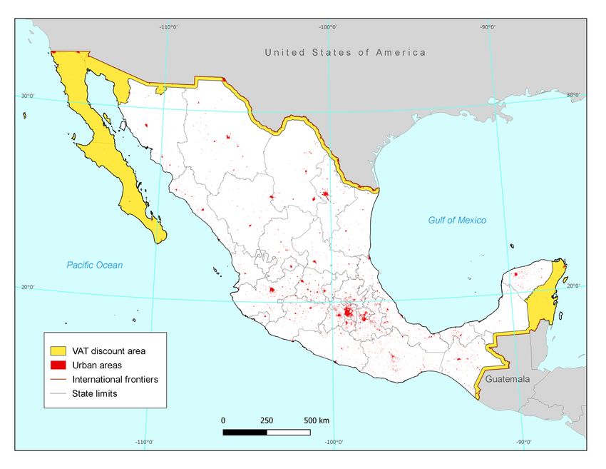
ary effects. We complement this literature by taking a different approach to measure the
effect of the VAT hike on prices. Instead of taking general inflation as outcome, we focus
on the prices of products and services that are treated by the reform, i.e. those that are
subject to the VAT. With this approach, we find a positive and lasting effect on prices.9 We
use the same approach to analyze the effect of the VAT reform on labor outcomes. This
appoarch allows to get a novel finding (the negavite effect of the reform on wages) for the
VAT incidence literature in Mexico.10

    To estimate the impacts of the VAT hike, we use two methods that are closely related: the
traditional “static” difference-in-difference (DiD) methodology, and also dynamic difference-
in-differences. The static DiD method gives a point estimate that we use to compare the
effects of the reform with the full pass-through counterfactuals. The dynamic DiD gives an
estimate for a given period of time that makes it possible to examine how the effect of the
reform is distributed in different periods. The area subject to the VAT discounted rate of 11
percent before the 2013 reform is mostly a 20 kilometer strip from the international frontiers.
The treatment group is composed of the municipalities where the majority of the population
lives in the VAT discount area.11 The control group is composed of the municipalities that
are located inside States at the international borders, but outside the VAT discount area.
In addition, as mentioned above, our estimation strategy takes into account the goods and
economic sectors that are subject to the VAT to estimate more precisely the treatment effect
on the treated.12
   9
      Our approach bears some resemblance to an estimation done by Campos-Vazquez and Esquivel (2020).
They study a package of tax and wage policy changes at Mexico’s northern border in 2018; among these, a
VAT cut. They find that the policy package did not have an effect on general prices (inflation). However,
the prices of groups of products prone to be taxed by the VAT were affected. Campos-Vazquez et al. (2020)
study the same policy package and find a positive effect on wages. We build on this research by isolating
the causal effect of the VAT on the Mexican labor market.
   10
      By focusing on the treated sectors, we extend evidence provided by Núñez Joyo (2017) on the effect of
the VAT hike on the labor market. Our research is in contrast with his findings as we find that the reform
had a negative effect on wages with no effect on employment.
   11
      We count with information at the municipality level for most outcomes. For estimation purposes, this
poses a problem, as the area of most municipalities at the international borders is not completely covered
by the 20 km strip. So, to define the treatment area, we analyze the geographic location of cities and rural
areas in each municipality. More information on this is provided in Section 4.
   12
      For the United States outcomes, we use the same difference-in-difference methodology, but we adapt
the treatment and control groups to each outcome. We describe this in detail in Section 5.2.

                                                     4
The reminder of the paper is organized as follows: in Section 2, we describe the 2013 tax
reform that included the VAT hike at the international borders; in Section 3, we describe the
data sources for the Mexico and United States outcomes; Section 4 describes the methodology
and the treatment and control groups we use in this study; Section 5 presents the results
and robustness tests; finally, Section 6 concludes.

2        The Value Added Tax Reform

The value added tax (VAT) was introduced in Mexico in year 1979. Since its origin, pol-
icy makers contemplated that the tax should be adapted to the particular context at the
borders, as it included a different rate in the localities at the frontiers (6 percent) and the
rest of the country (10 percent). The VAT rate has gone through several rate changes since
its creation.13 In 2013, the general VAT rate stood at 16 percent, with a smaller rate of
11 percent in a geographic area that mostly comprised a 20 kilometer strip from the in-
ternational borders. These rates were in effect since year 2010. In September 2013, the
President presented a tax reform to Congress that increased the VAT rate at the 20 km strip
to standardize the rate at 16 percent in all the country. This represents a 45 percent increase
in the previously discounted areas. The reform was approved by Congress in October, and
took effect in January 2014. It included several measures besides the VAT tax hike at the
international borders.14 All other measures were introduced in the whole country, so they
should be accounted for in the estimation strategy that we explain in Section 4. The main
justification the government used to introduce the 2013 tax reform was to increase tax col-
lection, as Mexico’s tax revenues are low, not only by OECD standards, but also compared
to other Latin American countries.15
    13
      In 1983, the VAT rate was raised to 15 percent in the whole country. In 1991, it was cut to 10 percent.
Then, in 1995 the VAT rate was raised to 15 percent but not at the international frontiers. For more
information see Mariscal and Werner (2018).
   14
      Among these are: measures to incorporate informal firms to the formal sector, a special tax on stock
exchange transactions, a slight increase in the income tax for the top brackets, a special tax on revenues of
mining companies.
   15
      In 2010, tax collection in Mexico (not including oil revenues) stood at nearly 14.5 percent of GDP.
The average in Latin America at that time was close to 19 percent of GDP. Meanwhile, the OECD average

                                                     5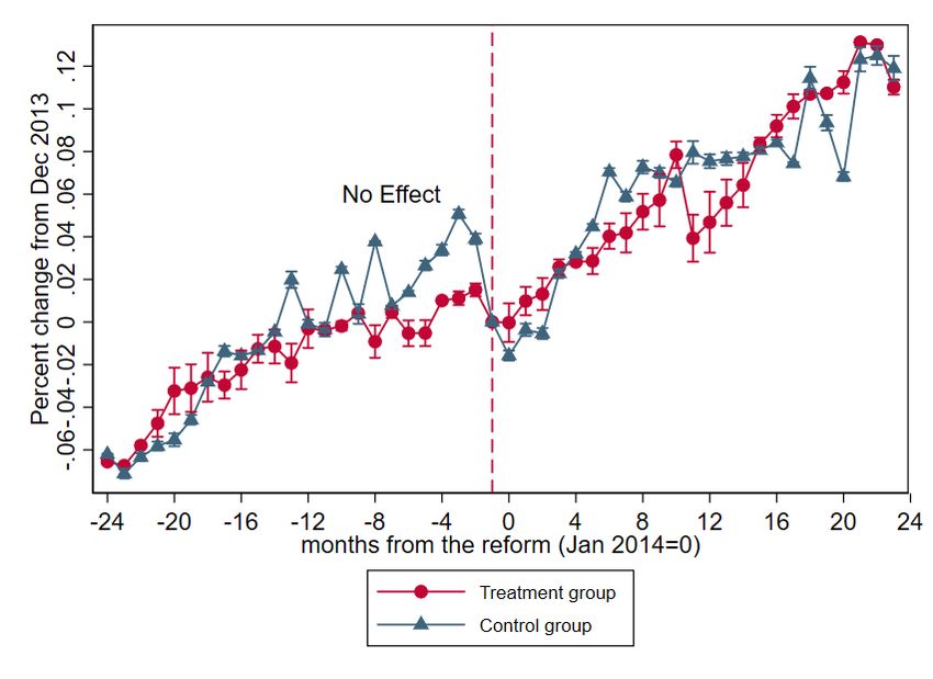
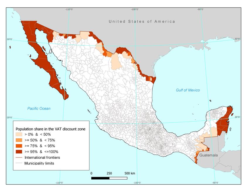
Figure 1 shows the VAT rate discount area before the 2013 reform. The area included
all localities situated at a distance of 20 kilometers or less from the international borders.
However, in some places, the discount area reached beyond the 20 km limit. Some states –as
well as some municipalities– were completely included in the VAT discount area.16 Around
9.9 million people lived in the VAT discount zone in 2010, i.e. nearly 9 percent of the
country’s population at the time. The VAT hike was greatly contested by numerous groups
at the international borders.17 The most vocal groups were business owner associations and
chambers of commerce. These groups organized demonstrations in bordering cities that at
some point registered attendances by the thousands.18 The main concern of these groups was
the loss of competitiveness relative to businesses at the other side of the international borders.
Specially in those of the US side, as the US sales tax in all bordering states stood below even
the discounted 11 percent VAT rate. However, some other concerns were mentioned. The
effects on inflation was one of these, but also the loss of employment. As firms would face
more costly inputs and loss of demand due to higher prices, they could be forced to cut on
employment. These concerns are outlined with detail in Fuentes et al. (2013). Despite the
unrest caused by the proposed bill, the VAT hike at the international borders was approved
by Congress without major changes.

3     Data

This research relies on multiple sources of administrative data collected both by Mexican
and United States agencies. Most datasets are publicly available. However, the datasets
collected by Banco de México and Comisión Nacional Bancaria y de Valores (CNBV) are
not (more on this below). Let us start by describing the Mexican datasets in this research.
stood at 26 percent (Clavellina-Miller et al., 2016). Arguably, the tax reform had some success in its goal to
increase tax collection. Tax revenues increased from an average of 14.2 percent of GDP in the three years
before the reform to an average of 17.3 percent of GDP in the three years after the reform (Clavellina-Miller
and Villarreal-Páez, 2016).
   16
      The exact locations subject to the discount zone are outlined in Cámara de Diputados del Congreso de
la Unión (2009).
   17
      https://elpais.com/internacional/2013/10/30/actualidad/1383116439 167910.html
   18
      https://www.jornada.com.mx/2013/10/20/politica/004n2pol

                                                      6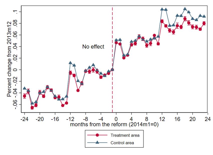
Data on prices comes from the Índice de Precios al Consumidor dataset collected by
Instituto Nacional de Estadı́stica y Geografı́a (INEGI). This dataset contains monthly in-
formation on prices of nearly 300 different products and services from 46 different cities
across Mexico. Of the Mexican datasets we use in this research, this is the only one that
provides data at the city level. The other datasets provide information at the municipality
level. We discuss the implications of this in Section 4. In addition, the prices dataset is the
most geographical constrained dataset that we use. For the other Mexican datasets, we have
information for most municipalities in the country.

    Data on labor outcomes comes from the Asegurados datasets collected by Instituto Mex-
icano del Seguro Social (IMSS). This dataset contains monthly information on the universe
of private employees in the formal sector at the municipality level. The dataset covers a
wide set of variables. In this research we are interested specially on two: mean wages and
employment level. A drawback of this dataset is that it only comprises the formal sector
of the economy. Mexico’s informal sector is quite large. It comprised about 60 percent
of total employment in 2013 (OIT, 2014). Nonetheless, the informal sector accounted for
just about 20 percent of GDP. Outcomes of the informal sector are usually analyzed with
Encuesta Nacional de Ocupación y Empleo (ENOE), an employment survey collected by
INEGI. However, this survey is not representative at the municipality level we use in this
research.

    Credit data comes from the datasets collected by Banco de México and shared with
Comisión Nacional Bancaria y de Valores (CNBV), both are the main financial market
regulators in the country. The datasets contain bimontly data on the universe of active non-
revolving consumer credits granted by financial institutions (commercial banks and Sofomes
R).19 A municipality level dataset of these credits is built using geographic information
   19
     Sofomes (Sociedades Financieras de Objeto Múltiple) are a specific kind of financial entity in the Mexican
financial regulation. These institutions are allowed to perform credit, leasing and factoring operations, but
they are not allowed to take deposits from the general public. Regulated Sofomes, or Sofomes R, are those

                                                       7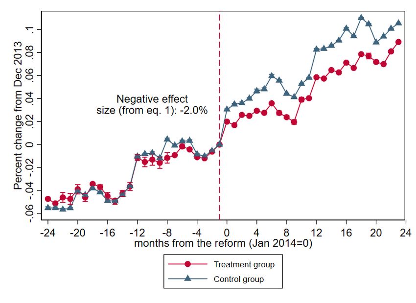
collected in the administrative reports. This dataset includes bimonthly information on
the number of new credits approved and the average interest rate of every approved credit
weighted by the credit amount at municipality level. For this work, only credits approved
during every two-month period are considered, as the conditions of credits active but ap-
proved before that period could be subject to different economic and financial contexts. In
this research, we are interested particularly on two types of credits granted to individuals:
1) payroll credits, i.e. credits that are discounted directly from workers’ payrolls, and 2)
credits granted specifically to purchase durable goods (designated as ABCD credits in the
Mexican context).20

    Moving on to the United States datasets. First, we use annual data on sales tax rev-
enues collected by the US Census Bureau. The data comes from the Annual Survey of
State and Local Government Finances. The survey covers all sources of revenues at the
state, county and city level. We use city level data. The survey covers all cities with popula-
tion larger than 70,000 inhabitants. In addition, we use monthly data on border crossings
collected by the Bureau of Transportation Statistics. The dataset contains information on
all entries to the United States at the port of entry level.21

4     Methodology

We use two methodologies to study the effect of the VAT hike at Mexico’s international
borders. First, we use the standard difference-in-difference (DiD) methodology described by
Angrist and Krueger (1999). We call this the “static” difference-in-difference. Second, we

that 1) have business activities involving financial holding companies and credit institutions, 2) fund their
securities operations using securities registered in the National Registry of Securities (RNV) kept by the
CNBV, or 3) voluntarily seek approval by the CNBV to be regulated. Most of these institutions are owned
or controlled by financial institutions.
   20
      ABCD credits, or Créditos para la Adquisión de Bienes de Consumo Duradero, are credits approved
by commercial banks and financial institutions with related retail stores which are granted the moment a
durable good is purchased. A durable good is expected to have longer life span than the credit term. This
commonly includes personal computers, televisions, and other household appliances.
   21
      Apart from the datasets mentioned above, we use INEGI’s Marco Geoestadı́stico and the US Census
Bureau’s TIGER/Line Shapefiles to create the treatment and control groups described in Section 4 and
Section 5.2, as well as the maps included in this paper.

                                                     8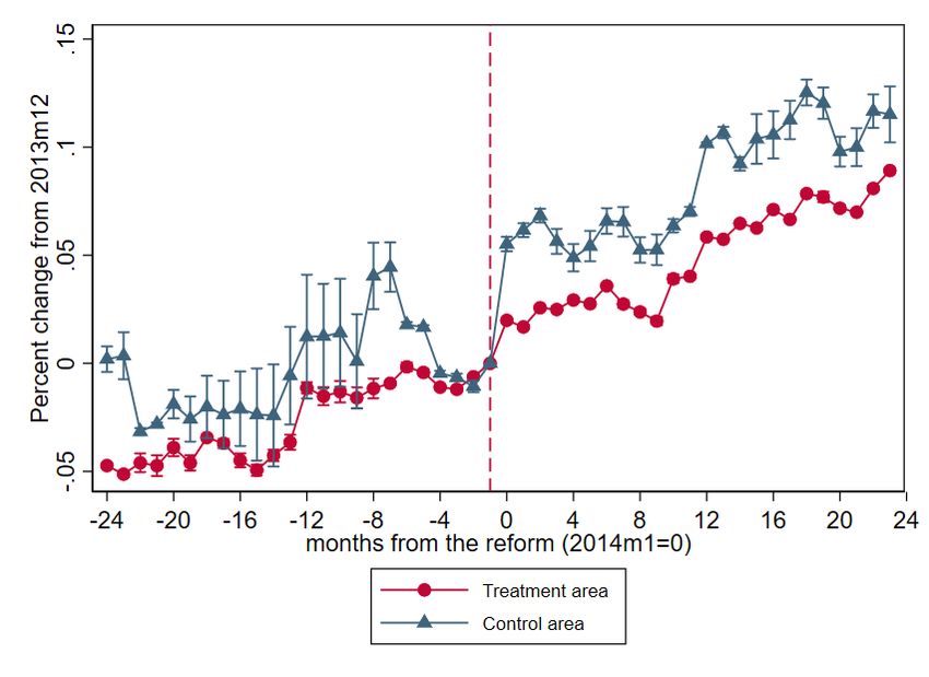
use the “dynamic” difference-in-difference methodology. The static DiD allows to get a point
estimate of the effect the policy. We use this point estimate to compare the effect of the
policy with the full-pass through counterfactual. The dynamic DiD shows the difference on
the outcome between treatment and control groups at a given point in time. This is useful
to examine if the policy has lasting effects in time and to confirm common trends prior to
the time when the policy takes place. A crucial part of this study is the definition of the
treatment and control groups, as both methodologies rely in defining a treatment group that
is subject to the policy change (i.e. the tax hike); and a control group that is not subject
to the policy change. Both groups must show common trends for the methodologies to be
valid. We explain in detail below the process we use to define the groups.

    The eligibility to the policy is conditioned to a geographic location. This location is
defined in Mexico’s value added tax law and shown in Figure 1.22 Using the geographic
delimitations in the law, we construct treatment and control geographic areas. The local-
ities that lie inside those areas are the treatment and control geographical units that we
use in our analysis. Most of the Mexican data we use in this analysis (except for prices) is
provided at the municipality level. The 20 km strip where the VAT discount rate applied
cuts through the area of most municipalities at the international borders. I.e. for most mu-
nicipalities at the border, a part of the territory lies inside the discount area and other part
lies outside. This brings particularities that must be treated carefully. If all the bordering
municipalities are included in the treatment group, one risks to include as treatment large
swats of economic activity that were not subject to the VAT discount before year 2014. This
would underestimate the true effects of the tax hike. So, to form our treatment group, we
keep the international bordering municipalities were the majority (50 percent or more) of the
population lives inside the VAT discount zone.23 These municipalities are shown in yellow
in Figure 2.
  22
     Cámara de Diputados del Congreso de la Unión (2009).
  23
     We use other population cut-offs for the treatment area: 1) municipalities where at least 75 percent of
the population lives inside the VAT discount area, and 2) municipalities where at least 90 percent of the
population lives inside that area. The population share in the VAT discount zone by municipality is shown
in Figure A6. We describe these alternative treatment areas with more detail in Section 5.3

                                                     9
The definition of the control area is also subject to considerations. The difference-in-
difference methodology is valid only if the treatment and control groups are in similar tra-
jectories prior to the policy change. We expect common trends in places that are close to
the treated municipalities. The area closest to the treated municipalities is composed of the
municipalities that are its immediate neighbors. However, focusing on just the immediate
neighbors for the control has some practical difficulties. As shown in Figure 2, the municipal-
ities that are contiguous to the treated municipalities contain relatively small urban areas.
Outcome information from these municipalities is sometimes absent and highly volatile, lead-
ing to imprecise estimates. To overcome this problem, we include municipalities with larger
populations in our control. So, we extend the control area to all municipalities in states at
the international frontiers where zero percent of the population lived at the VAT discount
zone prior to the 2013 reform. The control municipalities are shown in orange in Figure 2.24,25
The static DiD equation we use to estimate the effect of the 2014 VAT tax hike is:
Yjt = α + βMj + γDt + δMj · Dt + κt Tt + ΠXj · Tt + (1)
where Yjt is the selected outcome at municipality (or city for the price outcome) j and time
t. M = 1 if municipality j is in the treated area and M = 0 if municipality j is in the control
area shown in Figure 2. D = 1 if time t ≥ 2014 (the VAT hike took effect in January 2014),
and D = 0 otherwise. Tt are time dummies and Xj is a set of time-invariant municipality
24
Nonetheless, we estimate our regressions with two alternative control areas: 1) the municipalities that
are contiguous the treated municipalities, i.e., the “first degree neighbors” in Figure A7; and 2) the second
degree neighbors plus the first degree neighbors. We explain this with more detail in Section 5.3.
25
Table 1 shows the number of municipalities that count with information for each of the outcomes that
are related to workers’ purchasing power. Panel A shows the municipalities in the treatment area and Panel
B shows those of the control area. The price data is clearly the most restricted source of information that
we use in this paper. In the treatment area, 8 municipalities (cities) count with price information. On the
other hand, 65 municipalities have information on wages and employment. Nonetheless, the price data is
more stable. All municipalities with price data have information for all the time periods in our sample. In
the case of the labor outcomes, 90% (80%) of the municipalities with labor data in the treatment (control)
area have information for all the time periods. The relative scarcity of price data is another reason to extend
the control area to all municipalities in the States at the international borders (except for those at the VAT
discont zone).
10level controls interacted with time dummies. δ measures the effect of the VAT hike in the
outcome Y . The estimator obtained from equation (1) allows to get a point estimate of
the effect of the VAT hike on the outcomes we measure. In addition we use the following
equation to get the dynamic DiD estimators:
t=2015
X
Yjt = α + βMj + γt Tt + + δt Tt · Mj + ΠXj · Tt + jt (2)
t=2012
where Yjt is the outcome at municipality (city in case of prices) j and time t. M = 1 if
municipality j is in the treated area. M = 0 if municipality j is in the control area. Tt are
time dummies and Xj is a set of time-invariant municipality level controls interacted with
time dummies. In this specification, coefficients δt capture the difference in the outcome
between the treatment and control groups for a given time t.
The definitions mentioned above apply to all outcomes coming from Mexican data. The
outcomes that come from United States datasets follow the difference-in-difference estima-
tions of equations (1) and (2), but we define treatment and control groups with respect to
the United States context. We explain those groups with more detail in Section 5.2. We
estimate both the static and the dynamic DiD equations in the periods of time that com-
prise two years prior and after the VAT hike took place. The units of time differ across the
outcomes we analyse. We describe units of time when we explain our results in Section 5.
5 Results
We divide our outcomes in two categories: 1) internal outcomes, and 2) cross border shop-
ping outcomes. The internal outcomes comprise variables that affect workers’ real purchasing
power: prices, wages, employment and credits. For this set of outcomes, we analyze both
of Mexico’s international borders (in Mexico’s side of the border), i.e. the Mexico-United
States border and the Mexico-Guatemala/Belize border. The cross-border shopping out-
comes comprise variables that reflect shifts in demand across both sides of a border. For
11those outcomes, we focus only in the Mexico-US border (in both sides of the border) due to
more data availability in the United States relative to Guatemala and Belize.
5.1 Internal outcomes
We start by describing the effect of the value added tax hike that took effect in January
2014 on prices. This estimation has been previously done by Mariscal and Werner (2018).26
They estimate the effect of the 2014 VAT increase on the inflation rate. They find that the
reform had a positive but short lived effect. We propose a different approach to study the
effect of the VAT hike on prices as not all products and services in Mexico are subject to
the VAT.27 In general terms, the exemptions apply to food, non-alcoholic beverages, rent,
mortgages, medicines, medical consultations, public transport, books and private schooling.
So, taking the consumer price index (CPI) as outcome may underestimate the real effect
of the tax hike.28 To estimate the effect of the VAT increase on prices, our outcome is the
average price of the products and services subject to the VAT in the CPI dataset.29
Figure 3 shows graphical evidence on the of the VAT hike on prices. Panel (a) shows the
log change of the average price of goods subject to the VAT with respect to December 2013
–the period just before the VAT hike took place–. Before the reform, we see non statistically
significant differences on the log change in cities in both the treatment and control areas.
After the reform the log difference is clearly larger in treatment area compared to the control
area. Figure 3 shows that this effect is lasting in time. In addition, the figure includes the
estimate of δ from equation (1). The coefficient indicates that the VAT hike led to a 1.6
percent increase in prices as shown in column (1) of Table 2. The table shows estimates of
26
The control group in Mariscal and Werner (2018) is different than ours. We take as control the cities
that are outside the VAT discount zone and inside states at the international borders. They take as controls
all cities in Mexico that are outside the VAT discount zone.
27
This approach has been also used by Campos-Vazquez and Esquivel (2020) to show that a mix of policies
that included a VAT cut and minimum wage hikes in 2018 had an effect only on the prices of products subject
to the VAT.
28
Indeed, around 68% of the CPI is exempt of the VAT. This does not mean that 68% of the goods that
compose the CPI are VAT exempt. Rather, it means that 68% of the goods’ weights in the CPI are VAT
exempt.
29
The list of all products and services included in this average price is shown in Appendix B.
12equation (1) under three specifications: 1) without time dummies and control variables, 2)
with time dummies but no control variables, 3) with time dummies and control variables.30
In all specifications the estimate of δ is positive and significant. In addition, the size of the
effect is similar across specifications. Note that the VAT rate at the international borders
went from 11 to 16 percent in January 2014. Hence, a full pass-through of the tax change on
prices would amount to a price increase of about 3.6 percent.31 So, the effect of the reform
on prices is about half the size of the full counterfactual pass-through. This means that
business owners passed some of the tax increase to consumers, but not all. In addition, we
show the δt estimates from equation (2) in panel (b) of Figure 3. The figure shows that the
coefficients are not statistically different to zero prior to the VAT hike of January 2014. Af-
ter the reform takes place, the dynamic DiD estimates are positive and statistically different
from zero. These estimations reaffirm that the reform had a positive effect on the prices of
goods that are subject to the VAT.
For the labor outcomes, we carry an analysis similar to that of the price outcome. We
take the workers in firms that are part of sectors whose final products and services are subject
to the VAT.32 We construct the mean wage and the mean employment level in the treatment
and control municipalities from these sectors. Figure 4 shows graphical evidence on the effect
of the VAT hike of January 2014 on wages. Panel (a) displays the log change with respect
to December 2013. Before the reform, we see non statistically significant differences on the
log change in municipalities in the treatment and control areas. After the reform, the log
difference with respect to the December 2013 wage is larger in the control municipalities.
This indicates a negative effect of the VAT hike on wages of workers in sectors subject to the
VAT. The size of the effect from the static DiD estimator is around -2.0 percent as shown in
column (2) of Table 2. All specifications in the column are negative, significant and similar
30
Municipality level control variables include: the unemployment rate, the percent of the total workforce
employed in the formal sector, the total number of firms operating in a fixed address (public and private).
31
Take y as the price including VAT and x as the non-VAT price. Take t + 1 as the period after the VAT
change and t the period before the change. Then yt = 1.11x and tt+1 = 1.16x. The percent change in y
from period t to t + 1 is ∆%y = yt+1yt−yt × 100 = 1.16x−1.11x
1.11x × 100 ≈ 3.6.
32
These sectors are listed in Appendix B.
13in size.33 Note that the negative effect on wages is not as big as to lead to a wage decrease in
the treated areas. Rather, nominal wages increased, but more slowly than how they counter-
factually would. In addition, panel (b) of Figure 4 shows the dynamic DiD estimates from
equation (2). Prior to the reform the coefficients are not statistically different from zero,
whereas in all periods after the reform the coefficients are negative. This evidence reinforces
the negative effect of the VAT hike on wages.
Note that the VAT reform had an equalizing effect in terms of prices and wages across
the treatment and control areas. Panel (a) of Figure 5 shows the logarithm of the mean price
of goods subject to the VAT. After the VAT hike, mean prices in the treated cities start to
catch up with those of the control cities. Panel (b) of Figure 5 shows the logarithm of mean
wages of workers in sectors subject to the VAT. The figure shows that prior to the reform,
mean wage in the control municipalities was lower than that of the treated municipalities.
After the reform, wages in the control area raised more rapidly than those of the treatment
area, to the point were wages across both areas were not statistically different. So, the reform
appears to have erased the relative attractiveness of the border region in terms of prices and
wages.
Moving to the employment outcome, Panel (a) of Figure 6 indicates no clear evidence
on the effect of the reform on employment in sectors subject to the VAT. This is confirmed
in the results from equation (1) as shown in column (3) of Table 2. All coefficients in the
column are positive, but none is statistically significant. The series in Panel (a) of Figure 6
show large jumps in short periods of time, but the long term trends appear to move in par-
allel. To support the common trends assumption between the treatment and control groups,
we include in Panel (b) of Figure 6 the coefficients from the dynamic DiD regressions. The
figure shows that, before and after the reform, the DiD estimates are not statistically differ-
ent from zero. I.e., there is no effect of the reform on employment.
33
For the wage and the employment outcomes, municipality level control variables are the same that we
include in the price outcome. These are: the unemployment rate, the percent of the total workforce employed
in the formal sector, the total number of firms operating in a fixed address (public and private).
14Let us now discuss the findings on the price and labor outcomes that we have presented
so far. There is previous evidence of a VAT rate change that had an effect on wages. Ben-
zarti and Carloni (2019) find that a VAT cut in French sit down restaurants was shared with
employees in the form of higher wages (although most of the VAT cut went to higher business
profits). Our results support the finding that VAT rate changes have an effect on wages.
However, we find that the effect can go in a different direction. In the case we study here, a
VAT rate increase has a negative effect on workers wages. We do not think that this effect
is driven by workers moving between the treatment and control areas due to the reform. As
seen in Figure 6, the reform does not have an effect on the level of employment. In addition,
as shown in Panel (b) of Figure 4, mean wages are higher in the treatment areas compared
to the control areas before and after the reform. So, there is no wage incentive on workers
in the treatment areas to cross to the control areas around the time that the VAT reform
took place. Unfortunately, we do not count with information on profits to investigate the
effect of the VAT hike on that variable. However, evidence from previous literature shows
that businesses use prices to preserve or increase their profits when they face changes in the
VAT rate. In the context of our research, firms appear unwilling to increase prices to fully
compensate for the VAT rate hike. Likely, the reason being that they may lose demand to
firms at the other side of the international borders. Thus, in this context, firms appear to
adjust a part of the VAT hike (positively) on prices and another part (negatively) on wages.34
To complete our analysis on the effect of the VAT tax on workers’ purchasing power,
we estimate the effect of the VAT increase on payroll credits. These are credits that are
discounted directly from the workers’ payrolls. These credits are only granted to workers
employed in the formal sector, as banks link their collection to an official payroll. In the
CNBV datasets we cannot identify the economic sector of the firm where the credited worker
34
Note that wages did not nominally decrease. Rather, they did not increase as much as they would have
without the reform. This may have made it easier for firms to adjust on wages than to adjust on the level of
employment. Meaning that, firms continued to hire as they would have without the VAT reform, but paying
smaller wages than they counterfactually would.
15is employed. Thus, our treatment group is the payroll credits awarded in the treated mu-
nicipalities regardless of the worker’s economic sector of employment. Table 3 shows the
estimates of parameter δ for the static DiD model of equation (1). Column (1) shows the the
effect of the VAT hike on the number of new awarded payroll credits. The effect is negative
and significant in all specifications of the equation (1). Column (2) shows the effect of the
VAT hike on the average amount of these credits. All specifications are not statistically
different from zero. Finally, column (3) shows that the VAT hike did not have an effect
on the interest rate of these credits. Thus, according to these estimations, the reform had
a negative effect on the number of credits that workers contracted through their payrolls.
Although the average amount of the credits appears not to have changed. The negative
effect on the number of new payroll credits granted is not driven by changes in the nominal
interest rate. Figure 7 shows the estimates from the dynamic DiD model of equation (2).
Panel (a) shows these estimates on the number of new payroll credits granted. The figure
clearly shows that prior to the reform the DiD estimates are not statistically different from
zero. After the reform takes place, these estimates become negative. Panels (b) and (c) show
no effect of the reform on the average amount of these credits or on their interest rate.
To sum up this set of outcomes. The positive and lasting effect on prices indicates
that workers face higher prices due to the VAT reform –although these are smaller than
the full conterfactual pass-through–. In addition, workers have smaller wages than they
counterfactually would have had without the reform. On top of this, less credits are granted
to smooth out the harsher conditions brought by the reform. Our data does not allow to
tell if the negative effect on the number contracted credits is due to less credit applications
by workers or by more strict conditions to grant credits by banks. Nonetheless, the final
equilibrium result remains: workers face less opportunities to smooth out consumption in
face of the negative income shock caused by the VAT hike.35
35
In addition to payroll credits, workers can access credits through the regular “personal credits” granted
by Mexico’s financial institutions. Payment of these credits is not discounted from workers’ payrolls. These
credits are not only granted to workers; any adult individual can demand or be offered these credits. Panel B
of Table 3 shows the static DiD estimates on personal credits. The parameters are not significant either for
the number, the amount or the interest rate of personal credits. Figure A1 plots the dynamic DiD estimates.
165.2 Cross-border shopping
The 2014 VAT hike in Mexico’s cities close to international borders may have encouraged
consumers to travel to neighboring countries where consumption taxation is lower. In this
section we analyze these cross-border shifts in demand. We focus on the Mexico-United
States border due to more data availability to study changes in demand in the United States
side of the border, compared to the two neighboring countries of Mexico’s southern border:
Guatemala and Belize. Consumption taxes in the United States are collected via the sales
tax. This tax is set at the state and city level. The average sales tax rate in the four US
states that neighbor the Mexico’s northern border was lower than the 11 percent VAT rate
charged at Mexico’s side before the VAT reform.36
Let us start by studying changes in demand in Mexico’s side of the Mexico-US border.
The data we count with to analyze this is far from ideal, as we do not have information on all
consumption spending in the municipalities located in the treatment and control areas shown
in Figure 2. Instead, we count with a proxy of consumption via the number of new credits
granted specifically to purchase durable goods. These are credits that may be contracted
directly at the store where the durable good is purchased at the moment of the purchase.
In Mexico, all durable goods are subject to the value added tax. So, the VAT hike directly
affected all the goods that are purchased with these credits. Panel (a) in Figure 8 shows
the log change of the number of new credits granted to purchase durable goods in Mexico’s
northern border, both in the treatment and control municipalities. The figure indicates that
the VAT hike had a negative effect on the acquisition of these credits by consumers. This is
confirmed in panel (b) of figure 8 that shows the dynamic DiD estimates from equation (2).
Table 4 shows the static DiD estimates from equation (1). Column (1) shows that the VAT
The figure confirms that the reform does not have an effect on these credits. This means that the effect of
the reform on credits came from the payroll credits, i.e., those that just the workers on the formal sector can
be awarded with.
36
In year 2013, the average combined state and city sales tax rate in the four Mexico-US bordering states
was: 8.41 percent in California, 8.16 percent in Arizona, 7.26 percent in New Mexico and 8.15 percent in
Texas. In no city the combined state and city sales tax rate was equal or larger to the 11 percent VAT rate
charged at Mexico’s side of the border at that time. To this day, the combined state and city sales tax rates
in California, Arizona, New Mexico and Texas are lower than 11 percent.
17hike had a negative effect on the number of credits awarded to but durable goods. Columns
(2) and (3) show that there is no effect on the average amount of these credits or on their
interest rates.37 Thus, we find some evidence that of VAT hike having a negative effect on
the consumption of durable goods at Mexico’s side of the border. At least, on the durable
goods that are bought with credits.
We now study if some demand moved to the United States side of the border due to
the VAT hike. To do this, we use the same specification of equations (1) and (2), but with
different treatment and control groups. We start by studying the effect on sales tax collec-
tion in US cities. We analyze this outcome as changes in consumption in the US side of
the border should be reflected in the revenue collected from the sales tax. Figure 9 shows
the treatment and control groups for this outcome. The treatment group is composed of US
cities that lie at a distance smaller than 40 kilometers from the international border. The
40 km distance that we choose for the treatment area is set according to the distance that
Mexican nationals can travel into the United States with a Border Crossing Card (BCC).
BCC’s are special travel documents granted to Mexican nationals that reside near to the
border. The BCC allows its holder to visit US areas close to the border for up to 30 days
with no need to present a passport.38 The control group is composed of cities that lie in the
area that goes from a distance of 40 km from the border to 400 km. We take this distance
so that it resembles to the average distance of the control group in our Mexico’s outcomes
estimations.39
Panel (a) of Figure 10 shows graphical evidence on the effect of the VAT reform on sales
tax revenues in the US side of the border. In particular, it shows the logarithm of the mean
sales tax revenues in cities in the treatment and control areas. The figure shows no jumps
37
Dynamic DiD coefficents for these outcomes are shown in Figure A2.
38
Mexican nationals must apply for a visa in US consulates in order to visit the United States. Applicants
to US tourists visas must satisfy requirements that show their likeliness of not staying permanently in the
United States.
39
We use two alternative treatment areas: 1) US cities that are placed at the international frontier line,
and 2) US cities in the 40 km area that have a population of less than half the size of the closer Mexican
city at Mexico’s side of the border. More information on this is provided in Section 5.3.
18around the date the VAT hike took place. This depiction suggest that the reform had no
effect on sales tax collection. Panel (b) plots the dynamic DiD estimates from equation (2).
The plot shows no evidence of the the VAT hike having an effect on sales tax collection in
the Southern border of the United States. Static DiD estimates are shown in column (1) of
Table 5. All coefficients are not statistically significant. So, the analysis of sales tax revenues
in the United States indicates that the VAT reform did not lead to consumption shifting to
that country. Nonetheless, there is a number of problems with this variable. First, sales tax
revenues do not measure consumption directly, it is just a proxy of it to the extent that sales
tax collection moves in the same manner as overall consumption. Second, the variable is
collected in an annual basis. So, we cannot detect changes over smaller periods of time that
the reform may have had. Third, consumption of Mexicans in the US bordering cities may
be a very small share of overall consumption. So, our regressions may not be able to detect
changes in consumption by Mexicans if the outcome we use is related to overall consumption.
To reinforce our analysis on consumption in the US side of the border, we use an additional
outcome: land border crossings from Mexico to the United States. If the VAT hike pushed
Mexico’s residents at the border to buy more in the United States side, then we may expect
to see a higher number of crossings from Mexico to the US. The treatment group that we
use to study this outcome is the number of passengers that crossed the border using private
vehicles. Crossings for shopping purposes are registered in this category. The control group
is the number of containers that crossed to the US from Mexico by trucks.40 Panel (a) of
Figure 11 shows the log of the mean number of crossings in ports of entry at the Mexico-US
border. The figure shows no unusual jumps in the treatment or control group around the
time the VAT hike took effect. Panel (b) of this figure shows the dynamic DiD estimates.
The estimates are not statistically different from zero in all periods of time. This indicates
that the VAT reform did not have an effect on border crossings from Mexico to the United
States. The static DiD coefficients in column (2) of Table 5 is in line with this result.
40
We use additional treatment and control groups to study this outcome. We describe them with detail
in Section 5.3.
19Thus, from the outcomes we analyze in this paper, we find no evidence of the VAT reform
having an effect on consumption at the US side of the border. The absence of consumption
shifting to the United States could be due to legal barriers imposed on Mexicans in the form
of travel documentation requirements to cross the border. Indeed, Mexicans that reside at
the border can be denied of a Border Crossing Card (or a tourist visa) in the basis of income
or work status, among others. However, there is no evidence that restrictions on Mexicans
to cross to the US side where different before and after the reform. There may be legal
restrictions to cross the border, but a large number of Mexican nationals count with US
travel documents that allow a high degree of mobility across the border. So, other reasons
may explain the lack of evidence of increased shopping at the US side. From our analysis in
the internal outcomes in Mexico, we showed that the reform led prices to increase but only
by less than half of the full pass though counterfactual. So, prices increased after the VAT
hike but not by much. This small price increase may not have been enough to push Mexican
consumers to shift part of their consumption to the United States. In the cross-border
shopping literature this situation would be in line with a price increase in a jurisdiction not
being high enough to compensate for the costs of crossing to the neighboring jurisdiction. If
this was the case, we could deduce that firms at the Mexican side of the border saw a menace
in rising prices by a larger measure than they did, as the threat of loosing consumption to
the United States side is always looming.
5.3 Robustness
We begin by describing the robustness tests that we perform on the outcomes related to
workers’ purchasing power. First, we test if the VAT hike had an effect on prices and labor
outcomes in the sectors that are not subject to the VAT. These sectors do not receive the
treatment in both the treatment and control areas. So, they resemble a placebo group that
serves as a point of comparison with the treated group. Panel (a) of Figure A3 shows graph-
ical evidence on the effect of the VAT hike on prices of goods in these sectors. The figure
shows that the percent changes of prices among the treatment and controls areas are similar
20before and after the reform, i.e., there is no jump in the log change in the treatment area
at the time the reform takes place. This indicates that the reform did not have an effect
on the prices of goods that are not subject to the VAT. Panel (b) of Figure A3 plots the δt
parameters from the dynamic DiD. The figure confirms that the reform did not have an effect
on these prices, as the coefficients are not statistically different from zero before and after
the reform. In addition, Figure A4 shows that the VAT hike did not have an effect on the
wages of workers employed in these sectors. The same is true for the level of employment, as
shown in Figure A5. The static DiD estimates of these three outcomes are shown in Table
A1. Coefficients in all specifications are not statistically different from zero. The results
from these placebo tests give empirical support to the choice of our treatment and control
areas under the difference-in-difference empirical strategy. In Panels (a) of Figure A3 (non
treated prices) and Figure A4 (non treated wages) we see that, in the absence of treatment,
the pre-treatment and the post-treatment differences are the same. So, the common trends
assumption in which the difference-in-difference estimation relies is empirically supported.
The extra post-treatment difference that we see in Panels (a) of Figure 3 (treated prices)
and Figure 4 (treated wages) is caused by the VAT reform.
We also perform robustness tests with different treatment areas. In addition to our pre-
ferred treatment area,41 we perform the regressions with the following treatment areas: 1)
municipalities where 75 percent or more of the population lives in the VAT discount zone, 2)
municipalities where 95 percent or more of the population lives in this zone, 3) municipalities
where 50 percent or more of the population lives in this zone, but excluding those where
the majority of the population is located at a distance larger than 20 kilometers from the
international frontiers. The first two groups are included to check if the population share
cut-off that we choose affects our results.42 The purpose of the third group is to exclude
the places far from the international borders where the VAT had a discounted rate prior to
2014. As seen in Figure 1, some States where included completely in the VAT discount zone.
41
That is, municipalities where 50 percent or more of the population lives in the VAT discount zone, as
in Figure 2.
42
The municipalities included in each population share cut-off are shown in Figure A6.
21Some municipalities in these States had a VAT discount rate, but were located far from the
borders. The estimates from the static DiD equation (1) are shown in Table A2. Panel A
shows our baseline treatment area. Panels B, C and D show the alternative treatment areas.
The table shows that estimates of the effect of the VAT hike in the alternative treatment
areas, do not differ significantly from our baseline treatment. This is true for all outcomes
shown in the table: prices, wages, employment and payroll credits43 Thus, our results are
robust to different definitions of the treatment.
A different set of tests is related to the control area. We define two alternative control
areas: 1) the municipalities that are “first degree neighbors” of the municipalities in the
treatment area, i.e., the municipalities that are contiguous to those of the treatment area;
2) the municipalities that are “second degree neighbors” (those are contiguous to the first
degree neighbors) plus the first degree neighbors. These areas are shown in Figure A7. The
results from the static DiD estimator are shown in Table A3.44 Panel A shows our baseline
control area.45 Panel B shows the results with the first alternative control area. The estimate
of the effect on wages of workers employed in sectors subject to the VAT is negative but
not statistically significant. Panel C shows the results with the second alternative control
area. The wage estimate here remains negative and turns statistically significant at a 95
percent confidence level, but not at the 99 percent confidence level of our baseline control
area. As shown in Figure A7, a large share of the municipalities that are adjacent to the
treated municipalities have relatively small urban areas. Information from these sparsely
populated municipalities tends to show large variations and missing observations, and this
limits our ability to detect statistically significant effects.46 This problem can be seen in
43
Panels B and C in Column (1) show no information because all the cities for which we have information
on prices are located in municipalities where nearly all the population lives in the VAT hike area. So,
estimates from Panel B and C are the same of Panel A.
44
We focus on the labor outcomes for these robustness test because the cities for which we have price
data are two few to divide among alternative control areas. This can be seen in Table A4. Panel B shows
that no municipality in the first alternative control area has price information. Panel C shows that just four
municipalities in the second alternative control area count with price information. On the other hand, as
shown in Panel A, eleven municipalities in our baseline control area count with price information.
45
That is, all municipalities in States at the international borders where zero percent of the population
lives in the VAT discount zone, as shown in Figure 2.
46
Table A4 shows the number of observations by outcome under our baseline control area and the alter-
22You can also read