Relationship between Early-Stage Features and Lifetime Maximum Intensity of Tropical Cyclones over the Western North Pacific
←
→
Page content transcription
If your browser does not render page correctly, please read the page content below
atmosphere

Article
Relationship between Early-Stage Features and Lifetime
Maximum Intensity of Tropical Cyclones over the Western
North Pacific
Ren Lu and Xiaodong Tang *

                                          Key Laboratory of Mesoscale Severe Weather, Ministry of Education, and School of Atmospheric Sciences,
                                          Nanjing University, Nanjing 210023, China; mg1828011@smail.nju.edu.cn
                                          * Correspondence: xdtang@nju.edu.cn

                                          Abstract: The relationship between early-stage features and lifetime maximum intensity (LMI) of
                                          tropical cyclones (TCs) over the Western North Pacific (WNP) was investigated by ensemble machine
                                          learning methods and composite analysis in this study. By selecting key features of TCs’ vortex
                                          attributes and environmental conditions, a two-step AdaBoost model demonstrated accuracy of
                                          about 75% in distinguishing weak and strong TCs at genesis and a coefficient of determination (R2 )
                                          of 0.30 for LMI estimation from the early stage of strong TCs, suggesting an underlying relationship
                                          between LMI and early-stage features. The composite analysis reveals that TCs with higher LMI are
                                          characterized by lower latitude embedded in a continuous band of high low-troposphere vorticity,
                                          more compact circulation at both the upper and lower levels of the troposphere, stronger circulation at

                                   the mid-troposphere, a higher outflow layer with stronger convection, a more symmetrical structure
                                          of high-level moisture distribution, a slower translation speed, and a greater intensification rate
Citation: Lu, R.; Tang, X.
                                          around genesis. Specifically, TCs with greater “tightness” at genesis may have a better chance
Relationship between Early-Stage
                                          of strengthening to major TCs (LMI ≥ 96 kt), since it represents a combination of the inner and
Features and Lifetime Maximum
Intensity of Tropical Cyclones over
                                          outer-core wind structure related to TCs’ rapid intensification and eyewall replacement cycle.
the Western North Pacific. Atmosphere
2021, 12, 815. https://doi.org/           Keywords: tropical cyclone; lifetime maximum intensity; machine learning; AdaBoost; decision tree;
10.3390/atmos12070815                     composite analysis

Academic Editors:
Sundararaman Gopalakrishnan and
Ghassan Alaka                             1. Introduction
                                                Tropical cyclones (TCs), one of the most catastrophic weather events over the Western
Received: 26 May 2021
                                          North Pacific (WNP), have caused huge damage with strong winds and heavy precipitation
Accepted: 23 June 2021
                                          for decades [1,2]. Great effort has been put into improving TC intensity prediction for
Published: 24 June 2021
                                          a certain lead time through the development of statistical and dynamical models [3–8].
                                          However, there is a lack of research on influential factors of a TC’s lifetime maximum
Publisher’s Note: MDPI stays neutral
                                          intensity (LMI), a measurement related to its upper boundary of destructiveness.
with regard to jurisdictional claims in
                                                LMI might be affected by multiple factors during a TC’s lifetime, including its genesis
published maps and institutional affil-
iations.
                                          conditions. Previous studies on the physical mechanisms and favorable conditions of
                                          TC genesis have been conducted [9–13]. The genesis process of a TC can be divided into
                                          two consecutive stages [14,15]: first, from a tropical disturbance to a tropical depression
                                          (TD) with the formation of initial circulation; and second, from a tropical depression to
                                          a tropical storm (TS) when its warm-core structure is established. Gray [16,17] noted
Copyright: © 2021 by the authors.
                                          several favorable factors for TC genesis, including thermodynamic factors of sufficient
Licensee MDPI, Basel, Switzerland.
                                          ocean thermal energy, conditional instability throughout the low troposphere and high
This article is an open access article
                                          relative humidity in the mid-troposphere, and dynamic factors of a large enough Coriolis
distributed under the terms and
                                          parameter, above-normal low-level vorticity, and weak vertical wind shear near the center
conditions of the Creative Commons
Attribution (CC BY) license (https://
                                          of a TC’s circulation. He further emphasized the key roles of climate conditions (e.g.,
creativecommons.org/licenses/by/
                                          region, season, etc.), certain synoptic flow patterns (e.g., monsoon trough), and active
4.0/).                                    mesoscale convective systems (MCSs) in TC genesis. Based on that, the genesis potential

Atmosphere 2021, 12, 815. https://doi.org/10.3390/atmos12070815                                         https://www.mdpi.com/journal/atmosphere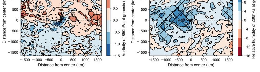
Atmosphere 2021, 12, 815                                                                                            2 of 28

                           index (GPI) [18,19] was developed to quantitively assess the probability of TC genesis at a
                           certain location, which suggests some key factors for LMI as well.
                                 In addition to the genesis conditions, the development stage also plays an important
                           role in determining LMI when a formed TC interacts with the environment and changes
                           its own structure. From the dynamic aspect, vertical wind shear is commonly detrimental
                           to TC intensification [20–22]; the interaction of a TC with an upper-level trough can
                           lead to intensification [23–25] and other factors such as the distribution of environmental
                           vorticity and a TC’s inertial stability can also influence TC intensification [26,27]. From
                           the thermodynamic aspect, variations of ocean surface temperature, heat content, and
                           exchange coefficients of air–sea fluxes can significantly affect a storm’s intensification
                           rate [28–32], and ambient dry air may inhibit TC intensification [33–35]. A TC’s internal
                           features and processes are also found to be associated with its intensity change. For
                           instance, a TC’s inertial stability contributes a lot to its growth by effective local warming
                           with cumulus convection [26,36]; distribution of rainfall and convection is related to a TC’s
                           rapid intensification (RI) [37,38] and the eyewall replacement cycles (ERC) can result in
                           re-intensification [39,40].
                                 For an individual TC, as the time and location of LMI are both uncertain, it is difficult
                           to “forecast” LMI using traditional numerical models. Considering that the two key
                           stages mentioned above (genesis and development) have a great influence on a TC’s
                           intensity change, LMI could be regarded as the result of various factors during these two
                           stages. Ditchek et al. [41] investigated the relationship between the maximum attained
                           intensity and the genesis environment of a TC over the North Atlantic (NA). They used a
                           stepwise regression method to select the most important genesis variables for LMI and then
                           established a linear function to assess their relationship. The regression had an overall R2 of
                           0.41, indicating that even if maximum attained intensity was not fully determined by a TC’s
                           genesis conditions, the relationship did exist. TCs reaching higher intensity are associated
                           with stronger, more compact low-level vortices, better-defined outflow jets, a more compact
                           region of high midlevel relative humidity, and higher water vapor content at genesis over
                           the NA.
                                 However, the corresponding relationship was never proved over the WNP, and the
                           issue is full of challenges, as TCs over the WNP are subjected to more complex environ-
                           mental factors (e.g., monsoon trough, monsoon gyre, etc.) [34,42,43]. For this reason, a
                           statistical model with better nonlinear fitting capability is required to explain the contri-
                           butions of factors to LMI over the WNP. Recently, machine learning methods have been
                           found to be capable of handling complicated issues in earth sciences [44–46]. For example,
                           K-means clustering is used to segment maps of radar echoes [47], decision trees work well
                           in classifying convection areas [48], and artificial neural networks (ANNs) are applied to
                           make short-term predictions of TC intensity [49]. Among these algorithms, decision tree
                           has an outstanding interpretability and can be easily utilized for classification or regression,
                           which is applicable to the LMI attribution issue here.
                                 The purpose of this study is to discover how much the LMI of TCs over the WNP is
                           related to their vortex attributes and environmental conditions near genesis, and search for
                           the key factors that will affect LMI. For this purpose, features of the vortex and environment
                           around TC genesis are firstly extracted using reanalysis and best track datasets, then the
                           relationship between these features and LMI is investigated by ensemble machine learning
                           methods for two separate steps (one for rough classification and the other for specific re-
                           gression). After the model’s parameters are well tuned, a composite analysis of the leading
                           features that have largest impact on LMI is conducted to find the distinctions between TCs
                           with different LMI. In Sections 2.1–2.5, we briefly describe the data source as well as the
                           ways to extract the features, and show the workflow of the whole model. The results of
                           the model fitting and composite analysis of features are presented in Sections 3.1 and 3.2.
                           Finally, an overall summary and a further discussion are provided in Section 4.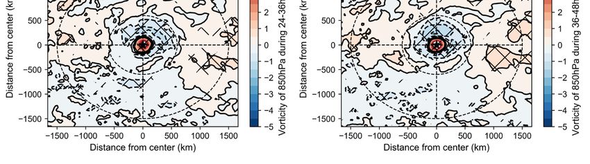
Atmosphere 2021, 12, 815 3 of 29
Atmosphere 2021, 12, 815
2. Materials and Methods 3 of 28
2.1. Data Source
Combining information from numerous TC best-track datasets, version 4.0 of the In-
ternational
2. MaterialsBest
and Track
MethodsArchive for Climate Stewardship (IBTrACS) [50–52] provides mul-
tiple attributes
2.1. Data Source of TCs (e.g., location, wind speed, translation speed, etc.) in every basin.
To avoid bias from
Combining datasets produced
information from numerous by different agencies
TC best-track as much
datasets, as possible,
version IBTrACS
4.0 of the
data of early-stage
International features
Best Track of storms
Archive over the
for Climate WNP basin
Stewardship from July
(IBTrACS) to November
[50–52] provides over 41
multiple
years attributesin
(1979–2019) of3TCs (e.g., location,
h intervals wind speed,
were obtained translation
from the Jointspeed,
Typhoonetc.)Warning
in every Center
basin. ToThese
(JTWC). avoidTCsbias are
from datasets
sorted intoproduced
3 groups byaccording
different agencies
to their as much
LMI: (1)asnever
possible,
intensified
IBTrACS data of early-stage features of storms over the WNP basin from July
beyond tropical storm (≤63 kt, TD/TS); (2) reached minor hurricane intensity but never to November
over 41 years (1979–2019) in 3 h intervals were obtained from the Joint Typhoon Warning
achieved major hurricane intensity (64–95 kt, minor TC); and (3) reached major hurricane
Center (JTWC). These TCs are sorted into 3 groups according to their LMI: (1) never
intensity (≥96 kt, major TC). TD/TS is also called weak TC and major/minor TC are col-
intensified beyond tropical storm (≤63 kt, TD/TS); (2) reached minor hurricane intensity
lectively named
but never achieved strong
majorTC. For convenience,
hurricane TCskt,
intensity (64–95 are labeled
minor TC);by their
and LMI level
(3) reached hereafter.
major
Environmental
hurricane intensity features aremajor
(≥96 kt, derivedTC).from
TD/TSERA5 hourly
is also calledreanalysis
weak TC and provided by the Euro-
major/minor
pean
TC areCentre for Medium-Range
collectively named strong TC. Weather ForecastsTCs
For convenience, (ECMWF),
are labeledwith a horizontal
by their LMI level resolu-
hereafter.
tion of 0.25° × 0.25°.
Environmental features are derived from ERA5 hourly reanalysis provided by
the European Centre for Medium-Range Weather Forecasts (ECMWF), with a horizontal
resolution
2.2. of 0.25◦of×the
Preprocessing
◦.
0.25Original Dataset
Preprocessing
2.2. Preprocessing ofOriginal
of the the TC Dataset
data was conducted to make the model work properly, in-
cluding spatial restriction
Preprocessing of the TCto data
focuswas on aconducted
certain scope of genesis
to make the modelandwork
temporal filtering to
properly,
remove short-lived TCs. First, the studied genesis area was restricted to a
including spatial restriction to focus on a certain scope of genesis and temporal filteringrectangular re-
gion over the
to remove WNP inTCs.
short-lived a range
First,of latitude
the studiedof 0–30°area
genesis N and
waslongitude 130–180°
restricted to E to exclude
a rectangular
region over
effects fromthe WNP
land in a range
during of latitude
the TC genesis 0–30◦ N
of stage and longitude
(Figure 1). Then, TCs ◦with
130–180 E to exclude
a lifetime less
effects
than 48from landremoved,
h were during thesince
TC genesis stagelonger
TCs with (Figurelifetimes
1). Then, TCs with a noteworthy
are more lifetime less than
in general.
48 h were removed, since TCs with longer lifetimes are more
The dataset was still large enough for traditional machine learning noteworthy in tasks
general. Theprepro-
after
dataset was still large enough for traditional machine learning tasks after preprocessing
cessing (Table 1) [53]. Further, information on features in each case was complete, so the
(Table 1) [53]. Further, information on features in each case was complete, so the model
model would not suffer from drawbacks caused by missing values.
would not suffer from drawbacks caused by missing values.
Figure 1. Illustration of studied genesis area (black rectangle) and eight storm-centered sectors where
Figure 1. Illustration of studied genesis area (black rectangle) and eight storm-centered sectors
variables are averaged. Red point is location of TC center, dashed blue lines are boundaries of four
where variables are averaged. Red point is location of TC center, dashed blue lines are boundaries
ofquadrants, and red and yellow circles represent radii of 600 km (inner circulation) and 1500 km (outer
four quadrants, and red and yellow circles represent radii of 600 km (inner circulation) and 1500
environment), respectively.
km (outer environment), respectively.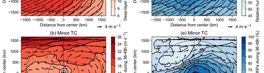
intensity, especially TDs (
Atmosphere 2021,
Atmosphere 12, x815
2021, 12, FOR PEER REVIEW 5 5ofof29
28
Figure 2. Box-and-whisker
calculation plots of (a)by
method introduced distance
Ditchek(km)etand (b) interval
al. [41], (hour) between
this method better locations
considersof the
TC
genesis and LMI over the WNP grouped by LMI level (yellow for TD/TS, orange
round shape of TC circulation, and features are independent of each other. Moreover, we for minor TC, and
red
alsoforfound
majorincluding
TC). Boxplot displays medianaverage
an axisymmetric (horizontal
(i.e.,black lineover
a circle nearthe
boxTCcenter), interquartile
center) as one of
range (box perimeter; [q1, q3]), whiskers (black lines; [q1–1.5 (q3–q1), q3 + 1.5 (q3–q1)]), and outliers
the features in the machine learning cannot change the results materially in terms of what
(rhombic points). The red horizontal line in (b) is a reference for the interval of 48 h.
variables are the most important for LMI, but otherwise performs badly on testing.
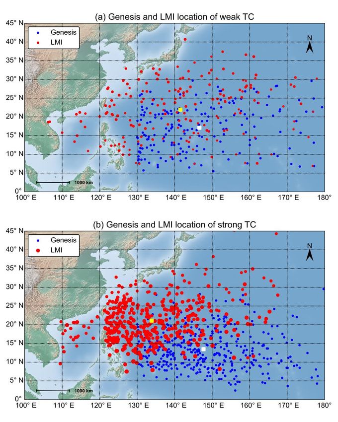
Table 2. Mean genesis and LMI locations of TCs and differences in two categories. All differences
Table 2. Mean genesis and LMI locations of TCs and differences in two categories. All differences of
of averages are significant at a confidence level of 99%.
averages are significant at a confidence level of 99%.
Weak TC Strong TC
Weak TC
Latitude Longitude Latitude Strong TC Longitude
Genesis Latitude
17.101° N Longitude
146.594° E Latitude
13.470° N Longitude
147.699° E
◦ 146.594E◦ E ◦ 147.699◦EE
LMI
Genesis 21.925° N N
17.101 141.508° 21.078°
13.470NN 133.890°
LMI
Difference 21.925◦ N
4.824° 141.508◦ E
−5.086° 21.078◦ N
7.608° 133.890◦ E
−13.809°
Difference 4.824 ◦ ◦
−5.086 7.608◦ ◦
−13.809
Figure 3. Locations of TC genesis (blue points) and LMI (red points) for (a) weak TCs (LMI of TD/TS)
Figure
and (b)3.strong
Locations
TCs of TC of
(LMI genesis
major(blue points)TCs).
and minor and LMI (red
White andpoints)
yellowfor (a) weak
squares TCs (LMI
indicate meanoflocations
TD/TS)
and (b) strong TCs (LMI of major and minor TCs). White and yellow squares indicate mean locations
of genesis and LMI, respectively. Size of each point indicates intensity (knots) at that time.
of genesis and LMI, respectively. Size of each point indicates intensity (knots) at that time.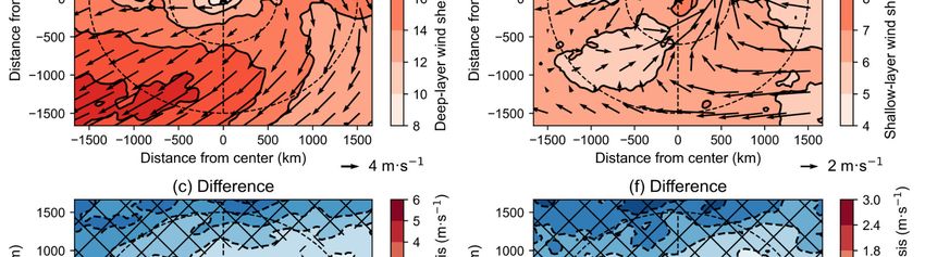
Atmosphere 2021, 12, 815                                                                                                            6 of 28

                                 Figure 2b shows the interval between TC genesis and LMI. The distribution is similar
                           to that in Figure 2a, indicating that generally the stronger the LMI, the longer the TC
                           interval. It is interesting that almost every strong TC (only 3 exceptional cases) experienced
                           a “developing stage” for at least 2 days before reaching LMI after genesis. For weak TCs,
                           the interval was quite short (e.g., less than 48 h for all TDs). Therefore, information from
                           the first 48 h is available to represent early-stage conditions of strong TCs.
                                 Similar to the process in the Statistical Hurricane Intensity Prediction Scheme
                           (SHIPS) [6,7,55], features are divided into 2 groups in this study: (1) TC state features,
                           which are scalars that describe the current status or variation trend of a TC such as size,
                           moving direction, and translation speed (Table 3); and (2) environmental features, which
                           are multidimensional variables that depict the dynamic or thermodynamic conditions of a
                           TC, such as air temperature, relative humidity, and vertical wind shear (Table 4). Some of
                           these parameters are crucial predictors in SHIPS for intensity prediction (e.g., SHRS and
                           SHRD) [55], and some have a huge impact on TC genesis (e.g., translation speed) [11,12,56].
                           All of them are derived from ERA5 hourly reanalysis and the IBTrACS dataset. The method
                           using reanalysis and actual best track data to establish a statistical model is known as the
                           “perfect prognostic” methodology [57].

                           Table 3. Variables used as TC state features in the model.

                                                   Variable                               Abbreviation                    Unit
                                    Day of year when TC generates *                            JDAY                        —
                                     Intensity variation in past 6 h **                         DV                        Knot
                                            Translation speed                                   SPD                       Knot
                                           Translation direction                                DIR                      Degree
                                            Coriolis parameter                                   F                      10−6 s−1
                                    Difference in Coriolis parameter **                          DF                     10−6 s−1
                                        Radius of maximum wind                                 RMW                        Km
                                          Radius of 3 m s−1 wind                                 R3                       Km
                                                 Tightness                                       TI                        —
                           * JDAY is made as a single feature since it does not vary with time. ** Due to the lack of TC information before
                           genesis in IBTrACS, DV, and DF are not included in the classifier (step 1).

                           Table 4. Variables used as environmental features in the model.

                                             Variable                       Abbreviation             Unit             Vertical Level
                                   Sea surface temperature                       SST                  ◦C                Surface
                                Maximum potential intensity                      MPI                 Knot               Surface
                                      Relative humidity                          RH                   %             200/500/850 hPa
                                       Air temperature                            T                   ◦C                200 hPa
                                       Relative vorticity                        VOR               10−5 s−1             850 hPa
                                         Divergence                              DIV               10−5 s−1             200 hPa
                                U-component of wind speed                         U                 m s−1               200 hPa
                              Vertical wind shear of deep layer                 SHRD                m s−1             200–850 hPa
                             Vertical wind shear of shallow layer               SHRS                m s−1             500–850 hPa
                             U-component vertical wind shear of
                                                                               USHRD                m s−1              200–850 hPa
                                          deep layer
                             U-component vertical wind shear of
                                                                                USHRS               m s−1              500–850 hPa
                                        shallow layer

                                 As for the variables mentioned in Table 3, each one is averaged every 12 h during the
                           first 2 days of a TC’s lifetime to be a feature, except for JDAY (absolute value of genesis
                           year-day minus 248). Specifically, the variables related to TC size are computed from 10 m
                           wind data from ERA5 [58], since the corresponding information in IBTrACS is incomplete.
                           In this way, the piecewise cubic Hermite interpolating polynomial (PCHIP) method [59] is
                           employed to extract the radius of 3 m s−1 wind speed (R3 ) and the radius of maximum wind
                           (RMW) from the storm-relative azimuthal-mean radial profiles. They represent the storm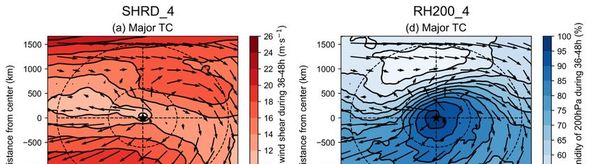
Atmosphere 2021, 12, 815                                                                                             7 of 28

                           sizes of the inner and outer core, respectively. Similar to the concept of TC fullness [60] as
                           the ratio of the TC’s outer-core wind skirt to outer-core size, tightness is calculated by:

                                                                R3 − RMW      RMW
                                                         TI =            = 1−     .                                     (1)
                                                                    R3         R3

                           By quantitively measuring the TC’s outer-core wind structure, this variable describes the
                           destructiveness of the storm to some extent.
                                Variables listed in Table 4 are also averaged within 8 sectors to be a feature in the model
                           after temporal averaging (Figure 1). The maximum potential intensity (MPI) used in this
                           study is calculated by an empirical function derived from the observed maximum intensity
                           of TC with respect to SST [55,61], rather than the theoretical form raised by Emanuel [62]:

                                                              MPI = A + BeC (T −T0 ) .                                  (2)

                                The coefficients in this exponential function are given by A = 38.21 kt, B = 170.72 kt,
                           C = 0.1909 C−1 , and T0 = 30.0 C−1 , and 185 kt is set as the upper boundary of MPI.

                           2.4. Ensemble Learning Method
                                The decision tree model mimics how people think about a problem and finally make
                           decisions, based on the rules organized in a tree shape [63]. It has a variety of forms, and
                           one of them is the classification and regression tree (CART), which typically uses the Gini
                           index as the rule to choose the best splitting feature at each node in classification [64]:

                                                                      K                       K
                                                      Gini ( D ) =   ∑ pk (1 − pk ) = 1 − ∑ p2k ,                       (3)
                                                                     k =1                   k =1

                                                                              V
                                                                                  | Dv |
                                                      Gini index ( D, a) =   ∑           Gini ( Dv ).                   (4)
                                                                             v =1 | |
                                                                                    D
                           where D and a refer to the original dataset and the selected feature, respectively, K is
                           the total number of features, V represents the number of possible values of a, pk is the
                           probability of the sample belonging to class k, and Dv is the subset split by a. The Gini index
                           shows the “impurity” of the subsets by calculating the possibility that two randomly chosen
                           samples in a subset have different actual labels. A low Gini index suggests that the subset
                           split by a is quite homogeneous, hence it is useful for classification [65]. After the training
                           is finished, the model will be able to classify new samples into certain categories by judging
                           their features step-by-step. CART can handle both classification and regression issues well,
                           with good capacity for interpretation, and acquires less training data than artificial neural
                           networks [66]. The detailed algorithms for CART are provided in Appendix A.
                                 Since a single decision tree is prone to overfit the training data by generating too many
                           branches [67], we use “pre-pruning” procedures (e.g., restricting the maximum depth of a
                           single tree) to prevent an unnecessarily complicated structure, and use ensemble to resist
                           overfitting. Ensemble learners contain sets of weak learners, and three ensemble learning
                           methods based on CART were applied in this study: Adaptive Boosting (AdaBoost),
                           Extreme Gradient Boosting (XGBoost), and random forest [68–70]. AdaBoost and XGBoost
                           are boosting models that train base models in series to reduce the bias by changing the
                           weight distribution of samples at each step. Random forest is a typical “bagging” algorithm
                           that has a parallel framework to reduce variance by constructing many decision trees. The
                           detailed algorithms for tree-based ensemble models are provided in Appendix B. Generally
                           speaking, ensemble learning methods are much more accurate and robust than individual
                           decision tree models [71,72].
                                 Similar to the individual decision tree model, the tree-based ensemble model not
                           only has good performance on classification and regression tasks, but is also available to
                           trace the contribution of each feature. Along with node division by the values of splitting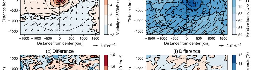
trees. The detailed algorithms for tree-based ensemble models are provided in Appendix
B. Generally speaking, ensemble learning methods are much more accurate and robust
than individual decision tree models [71,72].
Similar to the individual decision tree model, the tree-based ensemble model not only
Atmosphere 2021, 12, 815 has good performance on classification and regression tasks, but is also available to 8trace of 28
the contribution of each feature. Along with node division by the values of splitting fea-
tures, the decreased impurity in subsets is maximized at each step. Mean decrease impu-
rity (MDI)the
features, is employed
decreased to judge the
impurity in importance of feature at when
subsets is maximized the splitting
each step. point is
Mean decrease
set
impurity (MDI) is employed to judge the importance of feature xm when the splittingnodes
as s at node , whose value equals the mean decrease of selected metric over all point
and
is setallastrees
s at [70]:
node t, whose value equals the mean decrease of selected metric i over all
nodes and all trees [70]:
1
( )= ( ) ( )∆ ( , ), (5)
1
MDI ( xm ) =
NT ∑ w(Ti∈) ∶ ( )∑ p(t) ∆i (s, t) , (5)
Ti t ∈ Ti : v(st )= xm
where is the number of decision trees in ensemble model , ( ) is the fraction of sub-
where
set NT is
at node thea decision
t in number of decision
tree, ∆ ( , )trees refersintoensemble
the decreased T, p(t) is
modelimpurity the fraction
measured of
by the
subset atsplitting
selected node t incriterion, ( ) ∆i
a decision tree, s, t)weight
is (the refers toofthe decreased
decision treeimpurity
( ( )measured by the
≡ 1 in random
selected splitting criterion, w ( T ) is the weight of decision tree T (w (
forest), and ( ) is the value of the feature used in partition. Since we chose the Gini index
i i Ti ) ≡ 1 in random
forest),
as and v(stcriterion
the splitting ) is the value of models,
for all the feature weused in partition.
call the normalizedSince
MDI we the
chose theimportance
Gini Gini index
as the splitting criterion for all models,
index (GII; not the same as the Gini index). we call the normalized MDI the Gini importance
index (GII; not the same as the Gini index).
However, critical features assessed by only one criterion may be misleading, as the
However, critical features assessed by only one criterion may be misleading, as the
GII will be abnormally high when applied to high cardinality features [64]. To ensure the
GII will be abnormally high when applied to high cardinality features [64]. To ensure the
robustness of selected features, two other criteria, mean minimum tree depth (MMTD)
robustness of selected features, two other criteria, mean minimum tree depth (MMTD) and
and total split time (TST), are also considered quantitative indicators of feature im-
total split time (TST), are also considered quantitative indicators of feature importance. In
portance. In tree-based models, the earlier and more frequently a feature is selected, the
tree-based models, the earlier and more frequently a feature is selected, the more important
more important it is. Therefore, if the feature has a high GII, a small MMTD, and a large
it is. Therefore, if the feature has a high GII, a small MMTD, and a large TST, then it is
TST, then it is significant for LMI estimation.
significant for LMI estimation.
2.5.
2.5. Workflow
Workflow of
of the
the Model
Model
In
In order to better capture
order to better capture the
the detailed
detailed factors
factors of
of LMI
LMIfor forTCs
TCswith
withdifferent
differentintensity,
intensity,
we
we developed a two-step model to estimate the LMI of a formed TC based on
developed a two-step model to estimate the LMI of a formed TC based on aa classifier
classifier
and
and aa regressor
regressor (Figure
(Figure4).
4).The
Thefirst
firststep
stepofof
thethe model
model is judge
is to to judge whether
whether or not
or not a storm
a storm will
will become a strong TC by learning its genesis features (step 1). Since
become a strong TC by learning its genesis features (step 1). Since we are less interestedwe are less inter-
in
ested in the specific
the specific intensityintensity that TC
that a weak a weak
will TC willreach,
finally finallythereach,
nextthe
stepnext stepmodel
of the of thefurther
model
further
exploresexplores
the exact the exact intensity
intensity of strongofTCsstrong
onlyTCs only
(step 2), (step
where2), where during
features featuresthe
during the
first 48 h
first
after48 h afterare
genesis genesis are considered.
considered.
Figure 4.
Figure Flow diagram
4. Flow diagram of
of two-step
two-step LMI
LMI analysis
analysis in
in this
this study.
study. TD/TS is also
TD/TS is also called
called weak
weak TC
TC and
and
major/minor TCs are collectively named strong TCs.
major/minor TCs are collectively named strong TCs.
TC cases are randomly divided into two parts to establish the model: the training
set, used to tune the parameters of the model, and a testing set, used to evaluate its
performance. The ratio of the two subsets is 5/1 in this study. During the training process,
the three ensemble methods mentioned above are applied to the training set to tune its
critical parameters in the two steps (Appendix B). Meanwhile, k-fold cross-validation [73]
is applied to the training set to verify the capability of the model (k = 10 in this study). The
training set is divided equally into k subsets; then, training and testing are performed for k
iterations. During each iteration, one subset is selected for validation while the remaining
k–1 subsets are used to tune the parameters without overlap, so that each sample of the
dataset can be used for training and validation. Finally, the well-tuned model is assessed in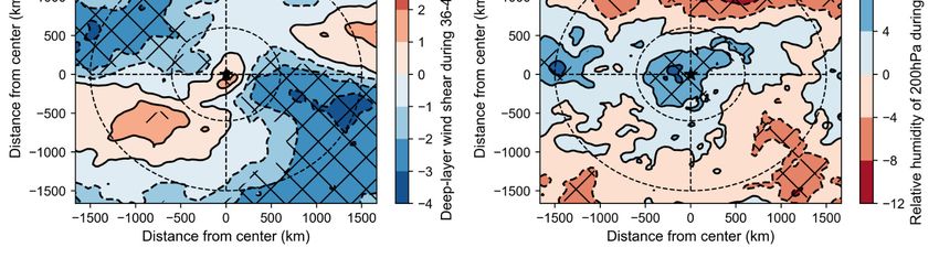
ing k–1 subsets are used to tune the parameters without overlap, so that each sample of
                           the dataset can be used for training and validation. Finally, the well-tuned model is as-
                           sessed in the testing set. In step 1, we use accuracy and F1-score as the metrics to evaluate
                           the fitting capability of classifier:
Atmosphere 2021, 12, 815                                                                                                   9 of 28
                                                                               +
                                                                  =                         ,                             (6)
                                                                         +     +      +
                            the testing set. In step 1, we use accuracy and F1-score as the metrics to evaluate the fitting
                            capability of classifier:                     2
                                                                 1 =          TP, + TN                               (7)(6)
                                                          Accuracy = 1 + 1                   ,
                                                                       TP + TN + FP + FN
                                                                              2
                                                                    F1 =  as:  ,
                           where P is precision and R is recall, calculated                                              (7)
                                                                            1    1
                                                                            P +  R

                                                                   =
                            where P is precision and R is recall, calculated   ,
                                                                               as:                                  (8)
                                                                          +
                                                                             TP
                                                                     P=             ,                                  (8)
                                                                          TP + FP
                                                                   =            .                                   (9)
                                                                          + TP
                                                                    R=               .                                 (9)
                                                                          TP + FN
                                The meanings of the double-letter variables in Equations (6)–(9) are explained in the
                                  The meanings of the double-letter variables in Equations (6)–(9) are explained in the
                           confusion matrix (Figure 5). Accuracy indicates the correctness of all decisions, and the
                            confusion matrix (Figure 5). Accuracy indicates the correctness of all decisions, and the
                           F1-score is a comprehensive term that judges the robustness of a classifier. The model will
                            F1-score is a comprehensive term that judges the robustness of a classifier. The model will
                           get a high F1-score only when precision and recall are both high, with precision measuring
                            get a high F1-score only when precision and recall are both high, with precision measuring
                           the quality of predicting true positive cases and recall measuring the completeness of the
                            the quality of predicting true positive cases and recall measuring the completeness of the
                           classifier’s judgment. In step 2, the coefficient of determination (R22) and root mean square
                            classifier’s judgment. In step 2, the coefficient of determination (R ) and root mean square
                           error (RMSE) are the two main metrics to evaluate the fitting capability of the regressor.
                            error (RMSE) are the two main metrics to evaluate the fitting capability of the regressor.

                           Figure 5. Confusion matrix with best score in testing set by AdaBoost classifier in step 1. Numbers in
                           squares indicate amount of corresponding TC cases. For both true and predicted value, 0 refers to
                           TD/TS (negative) and 1 refers to major TC/minor TC (positive).

                                After the three ensemble methods are well tuned for their optimum parameters, the
                           one showing the best performance on the testing set is selected as the benchmark in steps
                           1 and 2. To better understand the contributions of different features to the LMI of TCs,
                           the GII, MMTD, and TST of the benchmark are assessed to determine the most important
                           features. After that, the leading features are analyzed through storm-centered composites
                           of different LMI groups. Comparing their horizontal distribution and temporal variation
                           can show how the differences happen at the early stage of a TC’s lifetime.

                            3. Results
                            3.1. Features Related to LMI at TC Genesis
                                 In step 1, 111 features of 593 samples at genesis were applied to establish the classifi-
                            cation model distinguishing whether a storm will develop into a weak or strong TC, and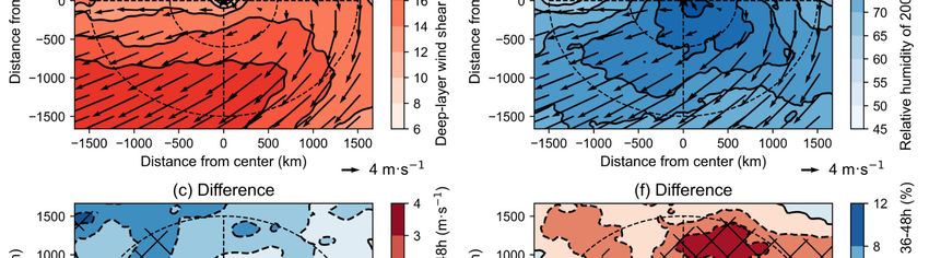
Atmosphere 2021, 12, 815 10 of 28
the fitting results for the three ensemble methods are shown in Table 5. It is clear in the
table that whether accuracy or F1-score is chosen as the criterion, the classifier based on
AdaBoost ensemble is ranked first (accuracy of 0.7479 and F1-score of 0.8387). It is also
optimum in terms of robustness (Appendix C). This suggests that a TC’s LMI is related to
its vortex attributes and environmental conditions at genesis over the WNP. As the aim
of this study is to discuss the impact factors of LMI rather than to provide operational
forecasting of LMI, the result of the AdaBoost classifier is good enough to ensure that the
following factor diagnosis is reliable. Therefore, it serves as the benchmark of step 1.
Table 5. Best results of fitting by three ensemble methods in steps 1 and 2.
Step 1 Step 2
Accuracy F1-Score RMSE (Knots) R2
AdaBoost 0.7479 0.8387 23.7697 0.3004
XGBoost 0.6975 0.8105 24.0103 0.2861
Random Forest 0.7227 0.8156 25.3060 0.2070
Figure 5 shows the confusion matrix of the result produced by the AdaBoost classifier.
It gets an F1-score of 0.839 with a high recall of 0.975 and a low precision of 0.736, mainly
caused by the large amount of FP cases (28 of 119). It is not surprising that the model
tends to overestimate the LMI of weak TCs but rarely underestimates that of strong ones.
Most TCs that form under favorable conditions suffer from disadvantageous factors after
genesis along their tracks (e.g., close to land) and will not attain a high LMI. However,
this situation cannot be captured by the model, since it learns information at genesis only.
Furthermore, the imbalance of the dataset induced by the relatively small proportion of
TD/TS cases (186 of 593) makes it harder for the classifier to learn the genesis features of
weak TCs. Nevertheless, the model does show some skill in classification.
The relative importance of features at genesis in step 1 assessed by GII, MMTD, and
TST is depicted in Figure 6; the most important features are highlighted by red points in
the upper left of the figure (MMTD ≤ 6.0, GII ≥ 0.015, TST ≥ 250) and ordinary features
are in blue. As the figure shows, TC vortex vorticity at genesis has the biggest impact
on LMI, with the most significant region northwest of the TC’s inner circulation. Vertical
wind shear of deep and shallow layers, relative humidity at the upper troposphere, and
translation speed at genesis are also key features. It is notable that two points in the lower
left of Figure 6 are far from the cluster (MPI_OUT_NW and USHRD_IN_NW), suggesting
that features judged by only one criterion may be misleading, so it is necessary to assess
their relative importance by multiple metrics.
3.1.1. Relative Vorticity at 850 hPa
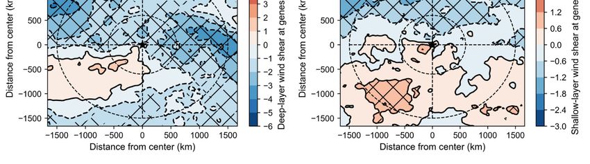
The most important feature in step 1, storm-centered composites of relative vorticity at
850 hPa in two groups and their differences, are shown in Figure 7a–c. For both weak and
strong TCs, the storm is situated in a continuous large vorticity band connecting to the west
(greater than 2 × 10⁻⁵ s−1 ), and the gradient near the storm center is also large. However,
as was found in NA [41], the eastern side of a weak TC’s outer environment is covered by
negative vorticity, with two features showing their evident difference (VOR850_OUT_NE
and VOR850_OUT_SE). Because most TCs over the WNP form to the south of the subtropi-
cal high, this suggests that TCs that reach high LMI tend to generate at a distance from the
subtropical high, or when it is weak.Atmosphere
Atmosphere2021,
2021,12,
12,815
815 1111ofof29
28
Scatterplot
Figure6.6.Scatter
Figure plotof of features
features at at genesis
genesis showing
showing their
their relative
relative importance
importance to LMI
to LMI in step
in step 1. x-1.
x- and y-axes refer to weighted mean minimum tree depth (MMTD) of all base
and y-axes refer to weighted mean minimum tree depth (MMTD) of all base estimators and Gini estimators and Gini
importance index (GII), respectively, with size of points controlled by total split time (TST)
importance index (GII), respectively, with size of points controlled by total split time (TST) in all in all trees
of the
trees ofensemble
the ensemblemodel. Red Red
model. points are features
points withwith
are features the greatest importance
the greatest importancejudged by the
judged bythree
the
three criteria,
criteria, and scatters
and blue blue scatters are ordinary
are ordinary features.
features. Textfeature
Text after after feature
namesnames in rectangles
in rectangles denotedenote
sectors
sectors indicated
indicated in Figure
in Figure 1. 1.
3.1.1. Relative
From theVorticity at 850
difference hPa
field (Figure 7c), we can detect a region with homogeneous
positive values of 0.5–1.0 × 10 −5 s−1 northwest of the TC’s inner circulation in accordance
The most important feature in step 1, storm-centered composites of relative vorticity
atwith
850 the
hPamost
in twoimportant
groups andfeature
theirindifferences,
step 1 (VOR850_IN_NW), and a 7a–c.
are shown in Figure regionFor
with negative
both weak
values at the southwest of the inner circulation. As the wind vectors
and strong TCs, the storm is situated in a continuous large vorticity band connecting show, the main
to
circulation of strong TCs (within a radius of 600 km) seems more symmetrical
the west (greater than 2 × 10⁻⁵ s−1), and the gradient near the storm center is also large. about the
zonal axisasthan
However, wasthat
foundof weak
in NATCs.[41],This
the might
easternbeside
a signal that storms
of a weak that environment
TC’s outer organize withisa
symmetrical circulation at genesis have a greater chance to reach higher
covered by negative vorticity, with two features showing their evident difference LMI.
(VOR850_OUT_NE
3.1.2. Local Verticaland
WindVOR850_OUT_SE).
Shear Because most TCs over the WNP form to the
south of the subtropical high, this suggests that TCs that reach high LMI tend to generate
Previous studies have recognized the remarkable impact of vertical wind shear on
at a distance from the subtropical high, or when it is weak.
the generation and intensity variation of TCs [20,74]. Figure 8 depicts the local vertical
From the difference field (Figure 7c), we can detect a region with homogeneous pos-
wind shear in two groups−5 and their differences. In terms of the local shear of deep layer
itive values of 0.5–1.0 × 10 s−1 northwest of the TC’s inner circulation in accordance with
(Figure 8a–c), the patterns in weak and strong TCs are quite similar, both characterized
the most important feature in step 1 (VOR850_IN_NW), and−1a region with negative values
by a narrow zonal band with low values about 8–10 m s across the storm center, and
at the southwest of the inner circulation. As the wind vectors show, the main circulation
higher values at the northern and southern sides. The most significant difference is the
of strong TCs (within a radius of 600 km) seems more symmetrical about the zonal axis
wider region of strong shear at the north and east of the storm in weak TCs, where the
than that of weak TCs. This might be a−signal that storms that organize with a symmetrical
maximum difference exceeds 4 m s 1 . Since there is little difference in wind fields at
circulation at genesis have a greater chance to reach higher LMI.
850 hPa (Figure 7a,b), this is mainly induced by the smaller range of anticyclonic flow to
the east of the storm center at 200 hPa in strong TCs. A more compact anticyclone nearer to
the storm center is observed in strong TCs, while in weak TCs the outflow extends farther
northward before wrapping back southward, leading to the ventilation of energy away
from the circulation [16]. Therefore, it can be inferred that a compact circulation in the
outflow layer at genesis is indicative of better conditions for TCs to attain higher LMI.
However, only one feature related to deep-layer shear is vital in step 1 (SHRD_IN_SE). This
may result from some extremes, which can dramatically influence the composite fields, but
the corresponding feature may be not indicative for classification.Atmosphere 2021,12,
Atmosphere2021, 12,815
815 12 of
12 of 28
29
Figure 7. Storm-centered
Figure 7. Storm-centeredcompositescompositesofof(a)(a)relative
relativevorticity (VOR850)
vorticity (VOR850) bybycontours with
contours withwind
wind vectors
vec-
at 850 − 5 − 1
tors athPa
850 (10
hPa (10s −5 s) −1and (d)(d)
) and relative humidity
relative humidity at 200 hPa
at 200 hPa(RH200)
(RH200) by by
contours with
contours withwind vectors
wind at
vectors
200 hPa
at 200 hPa(%)(%)
forfor
strong
strong TCs
TCsatat
genesis.
genesis.(b,e)
(b,e)are
arethe
thesame
sameasas(a,d),
(a,d),but
butfor
forweak
weakTCs.
TCs.(c,f)
(c,f) Difference
Difference
fields of
of strong
strong minus
minus weak weak TCs.
TCs. Black star represents storm center, and and dotted
dotted black
black lines
lines are
are
boundaries of eight sectorssectors discussed in FigureFigure 1. 1. Areas with crossing lines in in (c,f)
(c,f) depict
depict where
where
differences between
differences between two two categories
categories are
are statistically
statisticallysignificant
significantatatthe
the95%
95%confidence
confidencelevel.
level.
3.1.2.Both
Local Vertical
strong andWind
weakShear
TCs feature a cyclonic vortex in the middle layer of the tropo-
sphere, and there is a region with weak shallow-layer
Previous studies have recognized the remarkable wind shearofatvertical
impact the north of the
wind storm
shear on
center (Figure 8d,e). In terms of the wind shear of the shallow layer, SHRS_OUT_SW
the generation and intensity variation of TCs [20,74]. Figure 8 depicts the local vertical and
SHRS_OUT_NW
wind shear in twoare selected
groups andastheir
key features in step
differences. 1, which
In terms roughly
of the local conform to thelayer
shear of deep two
statistically
(Figure 8a–c), significant regions
the patterns in Figure
in weak and 8f. DueTCs
strong to the
aresimilarity in wind
quite similar, field
both at 850 hPa
characterized
between the two groups (Figure 7a,b), we attribute this difference to
by a narrow zonal band with low values about 8–10 m s across the storm center, and
−1 the storm’s circulation
at 500 hPa.
higher Comparing
values Figure 8d,e,
at the northern it is shown
and southern that The
sides. weakmostTCs significant
feature stronger southwest
difference is the
winds to the southwest of the outer environment and weaker easterlies
wider region of strong shear at the north and east of the storm in weak TCs, where to the north of the
the
storm center, which means the circulation in the middle layer is also weaker compared
maximum difference exceeds 4 m s−1. Since there is little difference in wind fields at 850
with strong TCs. As a result, weak TCs have a greater chance to draw in more dry air with
hPa (Figure 7a,b), this is mainly induced by the smaller range of anticyclonic flow to the
low potential vorticity at the middle level from the surrounding environment; hence, their
east of the storm center at 200 hPa in strong TCs. A more compact anticyclone nearer to
intensification is hindered [75].
the storm center is observed in strong TCs, while in weak TCs the outflow extends farther
northward before wrapping back southward, leading to the ventilation of energy awayfrom the circulation [16]. Therefore, it can be inferred that a compact circulation in the
outflow layer at genesis is indicative of better conditions for TCs to attain higher LMI.
Atmosphere 2021, 12, 815
However, only one feature related to deep-layer shear is vital in step 1 (SHRD_IN_SE).
13 of 28
This may result from some extremes, which can dramatically influence the composite
fields, but the corresponding feature may be not indicative for classification.
Figure 8. As in Figure 7, but for (a–c) deep-layer vertical wind shear (SHRD) of 850–200 hPa with
Figure 8. As in Figure 7, but for (a–c) deep-layer vertical wind shear (SHRD) of 850–200 hPa with
wind vectors at 200 hPa (m s−−11 ) and (d–f) shallow-layer vertical wind shear (SHRS) of 850–500 hPa
wind vectors at 200 hPa (m s ) and (d–f) shallow-layer vertical wind shear (SHRS) of 850–500 hPa
with −1
with wind
wind vectors
vectors at
at 500
500 hPa
hPa (m
(m ss−1).).
3.1.3. Relative Humidity at 200 hPa
Both strong and weak TCs feature a cyclonic vortex in the middle layer of the tropo-
Only
sphere, andone keyisfeature
there related
a region with to relative
weak humidity wind
shallow-layer (RH200_IN_NW) is selected
shear at the north of theinstorm
step
1, which indicates the valid difference in moisture conditions at the upper level of the
center (Figure 8d,e). In terms of the wind shear of the shallow layer, SHRS_OUT_SW and
troposphere between the two groups (Figure 7d–f). In general, there is little moisture at
SHRS_OUT_NW are selected as key features in step 1, which roughly conform to the two
the upper troposphere because ordinary convections can barely reach there [76]. However,
statistically significant regions in Figure 8f. Due to the similarity in wind field at 850 hPa
high relative humidity (nearly 100%) covers the storm center in both strong and weak TCs,
between the two groups (Figure 7a,b), we attribute this difference to the storm’s circula-
due to the low saturated water pressure. There are some similarities between TCs in the
tion at 500 hPa. Comparing Figure 8d,e, it is shown that weak TCs feature stronger south-
two groups. There is greater moisture to the south and its gradient is quite large at the
west winds to the southwest of the outer environment and weaker easterlies to the north
north of the storm center. However, moisture at the west of the storm center in weak TCs is
of the storm center, which means the circulation in the middle layer is also weaker com-
not as abundant as in strong TCs (the largest difference exceeds 12%), while strong TCs
pared with strong TCs. As a result, weak TCs have a greater chance to draw in more dry
have round-shaped and symmetrical wet areas around the storm center. In addition, the
gradient of relative humidity at the key region (northwest of a TC’s inner circulation) is
greater in weak TCs, which means the storm is embedded in a drier environment. This
difference implies that TCs with high LMI may have stronger and deeper convection at
genesis, which humidifies the outflow on the northwestern side.Atmosphere 2021, 12, 815 14 of 28
3.1.4. Translation Speed
The translation speed of storms is also found to be indicative in step 1. Overall, strong
TCs move a little slower than weak TCs at genesis (average speed 9.34 kt versus 10.35 kt),
and the difference is statistically significant at the 95% confidence level. This is contrary
to a previous study indicating that the enhancement of TC intensity is restrained by cold
water upward from the deep ocean due to the pumping effect when the storm remains in
a certain location for a long time [77]. On the other hand, TCs are usually formed in the
tropics with a warm underlying surface, so interaction with warmer seawater for a longer
time around genesis provides a better chance for the storm to gain heat flux from the ocean
and develop quickly. Moreover, since the study focuses on the early lifetime of TCs when
the wind speed of circulation is very low, the latter factor may have an advantage over the
former in affecting LMI. That is to say, TCs with a slower translation speed at genesis have
a greater chance to attain higher LMI.
3.1.5. Other Features
Some features related to the critical factors in the generation and intensity variation
of TCs are not selected in step 1 (e.g., SST, relative humidity at middle troposphere, di-
vergence at upper troposphere) because they do not differ much between the two groups.
Taking SST for instance, all of the TC cases investigated in this study form under similar
thermodynamic conditions of the ocean (Figure 3), so it is hard to distinguish their LMI
by features computed from a region-averaged SST. Similarly, MPI is also filtered by two
metrics, although it has a particularly small MMTD (Figure 6). This does not mean that it
does not contribute to TC genesis and intensity variation, but it is not a key feature affecting
LMI. A similar explanation may also be applied in step 2.
3.2. Features Related to LMI at Early Stage
In step 2, only minor and major TCs are investigated, and 449 early-stage features
of 407 samples are applied to establish the regression model (step 2) estimating the LMI
of strong TCs. The results of fitting by the three ensemble methods are shown in Table 5;
it is clear that the AdaBoost ensemble method again ranks first (RMSE of 23.7700 kt and
R2 of 0.3004). Figure 9 depicts the comparison between estimated and actual LMI in the
testing set, which resembles Figure 5 in Ditchek et al. [41]. The regression line of estimated
values has a smaller slope than line y = x, suggesting that step 2 is effective but has poor
performance on the extremes, similar to most machine learning models [78]. It implies
that the LMI of strong TCs could be affected by early-stage factors. Since we are seeking a
reasonable relationship between these factors and LMI rather than a perfect prediction, the
results produced by the AdaBoost-based model are considered credible and were used to
further discuss the relative importance of features.
As in Figure 6, the relative importance of features during the first 48 h after TC genesis
is depicted with GII, MMTD, and TST in Figure 10. Unlike the close positions of scatters in
Figure 6, the features in step 2 are dispersed in Figure 10 and have an approximately linear
distribution from the upper left to the lower right, suggesting that the key features selected
by the three metrics in this step are quite robust. Many TC state features are considered
to be crucial in step 2, which is a signal that vortex attributes of TCs begin to differentiate
during this period. On the other hand, the most critical environmental features are nearly
the same as those in step 1: deep-layer vertical wind shear, high-level relative humidity,
and low-level vorticity, with the key interval of 24–48 h after TC genesis. This implies
that these features have a great influence on LMI at the TC development stage as well as
at genesis.that the LMI of strong TCs could be affected by early-stage factors. Since we are seeking a
reasonable relationship between these factors and LMI rather than a perfect prediction,
Atmosphere 2021, 12, 815 the results produced by the AdaBoost-based model are considered credible and were15used of 28
to further discuss the relative importance of features.
Comparisonbetween
Figure9.9.Comparison
Figure betweenestimated
estimatedand
andactual
actualLMI
LMI(knots)
(knots)in inthe
thetesting
testingset,
set,colored
coloredaccording
according
toactual
to actualLMI
LMI(red
(redfor
formajor
majorand
andyellow
yellowfor
forminor
minorTC).
TC).Black lineisis y== x and
Blackline and blue
blue line
line isisregression
regression
Atmosphere 2021, 12, 815 16 of 29
line of
line of estimated
estimated values. Values of of metrics
metrics for
forevaluating
evaluatingfitting
fittingare
areininthe
thelower
lowerright.
right.Correlation
Correlationis
isstatistically
statisticallysignificant
significant
atat the
the confidence
confidence level
level ofof 99%.
99%.
As in Figure 6, the relative importance of features during the first 48 h after TC gen-
esis is depicted with GII, MMTD, and TST in Figure 10. Unlike the close positions of scat-
ters in Figure 6, the features in step 2 are dispersed in Figure 10 and have an approximately
linear distribution from the upper left to the lower right, suggesting that the key features
selected by the three metrics in this step are quite robust. Many TC state features are con-
sidered to be crucial in step 2, which is a signal that vortex attributes of TCs begin to dif-
ferentiate during this period. On the other hand, the most critical environmental features
are nearly the same as those in step 1: deep-layer vertical wind shear, high-level relative
humidity, and low-level vorticity, with the key interval of 24–48 h after TC genesis. This
implies that these features have a great influence on LMI at the TC development stage as
well as at genesis.
Figure10.
Figure AsininFigure
10.As Figure6,6,but
butfor
forfeatures
featuresduring
duringthe
thefirst
first48
48hhafter
aftergenesis
genesisin
instep
step2.2.
3.2.1. TC State Features
3.2.1. TC State Features
Variations of critical TC state features and differences between two groups during the
Variations of critical
first 48 h after genesis TC state features
are illustrated in Figureand11.differences
The averaged between two
Coriolis groups during
parameters of two
the first 48(24–36
intervals h after genesis
h and 36–48areh;illustrated
Figure 11a)inare
Figure
found 11.toThe averagedinCoriolis
be effective parameters
step 2 (F_3 and F_4).
of
It two intervals
can be (24–36
inferred h and TCs
that major 36–48 h; Figure
tend to stay11a)
in a are
lowerfound to bewith
latitude effective in step
a slower 2 (F_3
poleward
and F_4). It can be inferred that major TCs tend to stay in a lower latitude
motion, and the difference accumulates as time elapses (beyond 7.5 over 36–48 h). This with a slower
poleward
agrees with motion,
step 1,and the difference
in that accumulates
TCs with larger LMI spendas timemoreelapses
time (beyond 7.5 over
in the tropics 36–48
obtaining
h). This agrees with step 1, in that TCs with larger LMI spend more
energy from warmer seawater around genesis. As the difference in averaged translation time in the tropics
obtaining energy from warmer seawater around genesis. As the difference in averaged
translation speed between major and minor TCs gets bigger (0.5 m s−1 over 0–12 h but 0.78
m s−1 over 36–48 h after genesis, not shown), the difference in the Coriolis parameter also
becomes larger, making the feature indicative for LMI estimation.
Tightness has a similar increasing trend with the Coriolis parameter during the earlyAtmosphere 2021, 12, 815 16 of 28
Atmosphere 2021, 12, 815 17 of 29
speed between major and minor TCs gets bigger (0.5 m s−1 over 0–12 h but 0.78 m s−1 over
are more
36–48 likely
h after to go through
genesis, the RIthe
not shown), process, the result
difference in theindicates
Coriolisaparameter
key interval when
also most
becomes
major TCs will begin to intensify rapidly.
larger, making the feature indicative for LMI estimation.
Figure 11. Composite evolution of critical TC state features (blue and black lines) of (a) Coriolis
Figure 11. Composite evolution of critical TC state features (blue and black lines) of (a) Coriolis
parameter (F),
parameter (F),(b)
(b)tightness
tightness(TI),
(TI),and (c)(c)
and intensity variation
intensity in the
variation pastpast
in the 6 h (DV6) and their
6 h (DV6) and correspond-
their corre-
ing differences between major and minor TCs (red bars) during first 48 h after
sponding differences between major and minor TCs (red bars) during first 48 h after genesis. genesis. Except for
Except
first three intervals in (c), differences of all intervals are significant at a confidence level of 99%.
for first three intervals in (c), differences of all intervals are significant at a confidence level of 99%.
3.2.2.Tightness has aWind
Local Vertical similar increasing
Shear of Deeptrend with the Coriolis parameter during the early
Layer
lifetime of TCs (Figure 11b). As mentioned above, tightness is a term that describes the
Despite the lack of features describing shallow-layer shear, local wind shear of the
extent of a “valid” wind structure showing its destructiveness; a greater tightness value
deep layer is found to be critical in step 2 (SHRD_4_OUT_SE). There is no obvious differ-
(major TC) indicates a better-defined storm circulation. During this period, major TCs have
ence between composites of major and minor TCs (Figure 12a,b), both of which resemble
greater tightness than minor TCs, but the difference between the two decreases sharply
the genesis field in Figure 8a. The biggest difference (about 3 m s−1) at the southeast of the
at the interval of 24–36 h after genesis, possibly as result of the eyewall replacement cycle
outer environment is due to weaker deep-layer shear in major TCs. This difference isAtmosphere 2021, 12, 815 17 of 28
(ERC) process, which often takes place after a TC’s rapid intensification (RI; i.e., intensity
increasing more than 30 knots in 24 h). During the ERC process, the RMW of the storm
suddenly enlarges, leading to a decrease in tightness [40]. Among all the cases in step 2,
46 major TCs (17.97%) experienced RI during this period, but only 11 minor TCs (7.28%)
did, which supports our hypothesis. As a result, tightness at three intervals (TI_1, TI_2, and
TI_4) shows its importance to LMI at the early development stage of TCs over the WNP.
As for 6 h intensity variation, the difference between major and minor TCs is only
notable at the interval of 36–48 h (nearly 4.5 knots every 6 h), which is matched by a key
feature selected in step 2 (DV_4). During this period, major TCs keep developing fast,
but minor TCs have a drop in the intensification rate (from about 2.4 m s−1 to 2.2 m s−1 ),
which makes the difference suddenly increase (Figure 11c). Similar to the evolution of
tightness, this is probably related to the RI process. During 30–42 h after genesis, 47 major
TCs (18.36%) began to rapidly intensify, but only 9 minor TCs (5.96%) did. Because major
TCs are more likely to go through the RI process, the result indicates a key interval when
most major TCs will begin to intensify rapidly.
3.2.2. Local Vertical Wind Shear of Deep Layer
Despite the lack of features describing shallow-layer shear, local wind shear of the deep
layer is found to be critical in step 2 (SHRD_4_OUT_SE). There is no obvious difference
between composites of major and minor TCs (Figure 12a,b), both of which resemble the
genesis field in Figure 8a. The biggest difference (about 3 m s−1 ) at the southeast of the
outer environment is due to weaker deep-layer shear in major TCs. This difference is
mainly caused by the weaker anticyclonic flow at 200 hPa of major TCs, since the difference
in the wind field at 850 hPa is very small between the two groups (Figure 13d,e). Since
the difference takes place around genesis, this may result from the faster organization of
deeper convection and higher outflow layer by major TCs.
3.2.3. Relative Humidity at 200 hPa
Figure 12d,e respectively depict the composite fields of relative humidity at 200 hPa
of major and minor TCs, and Figure 12f shows their difference. Except for the wetter
environment around the storm center, major TCs have similar moisture distribution to
minor TCs. As implied by the key feature of RH200_4_OUT_NE, there is a key region
northeast of a TC’s outer environment for LMI (the biggest difference exceeds 8 m s−1 ).
Here, the environmental air of major TCs is extremely dry, where the gradient of relative
humidity reaches its maximum. This could be the consequence of stronger compensating
subsidence in the environment. Meanwhile, the anticyclonic circulation of major TCs is
also stronger. These characteristics imply that the upper-layer structure of major TCs
is more compact, with higher inertial stability, which is favorable for TCs to intensify
continuously [36]. This difference is not obvious in the genesis field when the circulation is
not well established.
3.2.4. Relative Vorticity at 850 hPa
There are two key features describing the low-level vorticity of TCs in step 2 (VOR850_
3_OUT_NE and VOR850_4_OUT_NE). Since they are calculated from two successive inter-
vals, their composites and difference fields are quite similar (Figure 13a,b,d,e). Similar to
the situation in genesis fields, stronger TCs are situated in more continuous vorticity bands
with greater convergence of southwest wind and easterlies to the east of the storm center.
There are two significant regions with large values in the difference fields (Figure 13c,f):
a negative one lying in the inner circulation around the storm center, and positive one
at the east of the outer environment. The former can be explained by the fact that major
TCs usually have a smaller inner core than minor TCs. Therefore, the difference fields are
covered by positive values within a radius of about 200 km, but the values outside are
negative. As a result, the mean vorticity of the inner circulation is similar in the two groups;
thus, the corresponding features are not selected in step 2. The latter region could beYou can also read