Wind speed and direction estimation from wave spectra using deep learning
←
→
Page content transcription
If your browser does not render page correctly, please read the page content below

Atmos. Meas. Tech., 15, 1–9, 2022
https://doi.org/10.5194/amt-15-1-2022
© Author(s) 2022. This work is distributed under
the Creative Commons Attribution 4.0 License.

Wind speed and direction estimation from wave spectra
using deep learning
Haoyu Jiang1,2,3
1 Hubei Key Laboratory of Marine Geological Resources, China University of Geosciences, Wuhan, 430000, China
2 Laboratoryfor Regional Oceanography and Numerical Modeling, Pilot National Laboratory for Marine Science and
Technology (Qingdao), Qingdao, 266000, China
3 Southern Marine Science and Engineering Guangdong Laboratory (Guangzhou), Guangzhou, 511458, China

Correspondence: Haoyu Jiang (haoyujiang@cug.edu.cn)

Received: 11 September 2021 – Discussion started: 15 September 2021
Revised: 26 November 2021 – Accepted: 28 November 2021 – Published: 3 January 2022

Abstract. High-frequency parts of ocean wave spectra are          high accuracy. However, the deployment and maintenance
strongly coupled to the local wind. Measurements of ocean         of these buoys and platforms usually have relatively high
wave spectra can be used to estimate sea surface winds. In        costs. Therefore, meteorological buoys are very sparsely dis-
this study, two deep neural networks (DNNs) were used to es-      tributed and are mostly only available along the coastlines of
timate the wind speed and direction from the first five Fourier   developed countries.
coefficients from buoys. The DNNs were trained by wind               The Earth observation satellite network, such as scat-
and wave measurements from more than 100 meteorological           terometers, altimeters, and synthetic aperture radars, can
buoys during 2014–2018. It is found that the wave measure-        serve as effective complements for the buoy network. Mean-
ments can best represent the wind information about 40 min        while, these remote sensors also have some limitations. Scat-
previously because the high-frequency portion of the wave         terometers can retrieve both wind speed and wind direction
spectrum integrates preceding wind conditions. The overall        with a wide swath and the best overall accuracy, but wave
root-mean-square error (RMSE) of estimated wind speed is          information is not available from them. Besides, their tem-
∼ 1.1 m s−1 , and the RMSE of the wind direction is ∼ 14◦         poral resolutions (usually one or two revisits per day except
when wind speed is 7–25 m s−1 . This model can be used not        for polar regions) are still much lower than those of in situ
only for the wind estimation for compact wave buoys but also      measurements. Altimeters can simultaneously measure wind
for the quality control of wind and wave measurements from        speed and significant wave height (SWH), but wind direc-
meteorological buoys.                                             tions and other wave parameters are not available from them.
                                                                  Besides, the cross-track spatial coverage and temporal res-
                                                                  olution of an altimeter are low because they can only mea-
                                                                  sure the nadir. Synthetic aperture radars’ wave mode can pro-
1   Introduction                                                  vide wind speed, wind direction, SWH, and low-frequency
                                                                  wave spectra (high frequency is not available due to nonlin-
Sea surface wind and waves are important parameters for           ear imaging), but the accuracy of wind speed, wind direction,
the marine environment and ocean dynamics. High-quality           and SWH is usually not as good as that from scatterometers
simultaneous measurements of sea surface wind and wave            and altimeters, and they are also limited by the sparse sam-
information are helpful for the study of many oceanic             pling. Moreover, spaceborne remote sensors often perform
and coastal phenomena. Such simultaneous measurements             worse in nearshore regions than in the open ocean due to the
can be obtained from meteorological buoys and remote              land contamination of backscatter.
sensing satellites. Many meteorological buoys can provide            Another important data source for collocated winds and
comprehensive wind and wave information, such as sur-             waves is compact wave buoys. These types of buoys are usu-
face wind speeds, wind directions, and wave spectra, with

Published by Copernicus Publications on behalf of the European Geosciences Union.
2                                                       H. Jiang: Wind speed and direction estimation from wave spectra

ally low-cost and are suited for deployment in large num-       every 10 min with a sampling time of 8 min and accuracy
bers, and they perform better in measuring waves com-           within 1 m s−1 and 10◦ for wind speed and direction, re-
pared to large meteorological buoys because their small sizes   spectively, in a moderate sea state (in extreme sea states, the
have a more sensitive response to short waves (Voermans et      swing and tilting of the buoy can introduce larger errors).
al., 2020). Although wave buoys are not designed for wind       The wind speed was converted to the standard height of 10 m
observation, Voermans et al. (2020) have shown that both        (U10 ) using the power law (Hsu et al., 1994) that was also
wind speed and wind direction can be estimated from the         used in Voermans et al. (2020). This conversion was also
wave spectra using an f − 4 spectral dependence in the equi-    tried using the log profile (Young et al., 1995), which has
librium range. Their model can estimate wind speed with a       almost no impact on the results. The waves are measured ev-
root-mean-square error (RMSE) of 2 m s−1 and wind direc-        ery 1 h with a sampling time of 20 min. The buoy wave data
tions with an RMSE of ∼ 20◦ when wind speed is higher than      include five Fourier coefficients of waves for different fre-
10 m s−1 . Although this model has good theoretical support,    quencies in the range of 0.02–0.485 Hz (47 frequency bins)
its accuracy is lower than typical remote sensing retrievals.   derived from the translational or pitch–roll information from
For example, altimeter-retrieved wind speed has a typical       the accelerometers and inclinometers on board buoys (Steele
overall RMSE of 1.2–1.5 m s−1 (e.g., Jiang et al., 2020) and    et al., 1998). The five Fourier coefficients are wave variance
scatterometer-retrieved wind speed and wind directions have     spectral densities (E) which describe the wave energy for
a typical overall RMSE of ∼ 1 m s−1 and 15◦ (e.g., Wang et      each frequency, mean and principal wave directions for each
al., 2021) when using buoys’ anemometer data as the refer-      frequency (α1 and α2 ), and first and second normalized po-
ence.                                                           lar coordinates of Fourier coefficients (r1 and r2 ) which de-
   Compact wave buoys are increasingly widely used in           scribe the directional spreading about the main direction for
global wave observations. For example, more than 2000           each frequency. The five Fourier coefficients of different fre-
Spotter buoys have been deployed in global oceans by So-        quencies are the minimum requirement to reconstruct the di-
far Ocean Technologies (the location of these buoys can         rectional wave spectrum. These NDBC data, especially the
be viewed at https://weather.sofarocean.com/, last access: 22   offshore data, are widely used in the validation of wind and
December 2021) to improve the performance of their wave         wave remote sensing and numerical weather and wave mod-
modeling (Smit et al., 2021). Although the data are not open    els (e.g., Jiang et al., 2016; Jiang, 2020; Wang et al., 2021).
to the public, more accurate wind estimation from wave spec-    The wave data and the wind data were collocated if their ends
tra can definitely benefit users of such buoys. Voermans et     of sampling time were within 10 min (the sampling duration
al. (2020) have shown the possibility of estimating wind        is ∼ 20 min for wave measurements and ∼ 10 min for wind
speed and wind direction with wave measurements alone.          measurement).
This study aims to improve the accuracy of such estimation
as much as possible. A model based on a deep neural network     2.2   DNN models for estimating wind speed and
(DNN) is presented to achieve this goal. The rest of this pa-         direction
per is organized as follows: the simultaneous observations of
wind and waves to train the DNN model are introduced in         As a nonparametric model, a DNN can theoretically be used
Sect. 2, along with the structure and training method of the    to fit any form of function with any number of input param-
DNN. The main results are presented in Sect. 3. A brief dis-    eters provided the network is wide and deep enough. The
cussion about the selection of the DNN input terms is given     DNN has been proved to be effective for regression prob-
in Sect. 4, followed by the concluding remarks in Sect. 5.      lems with more than two input parameters and is widely
                                                                used in the training of retrieval models and correction models
                                                                in studies of ocean remote sensing (e.g., Wang et al., 2020;
2     Data and methods                                          Jiang et al., 2020). A DNN is a useful tool for the problem
                                                                that there are causal relationships between inputs and outputs
2.1    Collocated wind and wave data                            (in this study, wave spectra and winds, respectively), but the
                                                                explicit form of the relationship is not known. In this study,
Many buoys from the National Data Buoy Center (NDBC)            two DNNs were established with the same structure, one for
coastal marine automated network can provide quality-           estimating wind speed and one for wind directions. In the be-
controlled in situ wave and wind measurements. The data         ginning, the input layer of the DNN, which simply contains
used in this study are the NDBC buoy data archived in           235 (vectorization of 5 Fourier coefficients × 47 frequency
National Centers for Environmental Information where the        bins) neurons, was set up in a “violent” way. However, we
data are available in NetCDF form. After removing the data      will show in Sect. 4 that the input layer of the DNNs can
records with bad-quality flags, more than 1.6 million records   be refined after obtaining the basic knowledge of how these
from 101 buoys in coastal and oceanic regions during 2014–      models work. Each of the 235 inputs was normalized to have
2018 were used in this study (Fig. 1). Most buoys’ anemome-     zero mean and unit variance. The DNNs have two hidden
ters are 4–5 m from the sea surface, and winds are measured     layers with 64 neurons followed by an output layer with one

Atmos. Meas. Tech., 15, 1–9, 2022                                                    https://doi.org/10.5194/amt-15-1-2022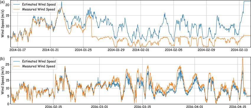
H. Jiang: Wind speed and direction estimation from wave spectra 3
Figure 1. The bias (a, b, c) and RMSE (d, e, f) of DNN-estimated wind speed and RMSE of DNN-estimated wind direction (when wind
speed is higher than 7 m s−1 , g, h, i) for the individual NDBC buoys in the North Pacific (a, d, g), the west coast of the United States (b,
e, h), and the Atlantic region (c, f, i). The overall RMSEs of wind speed and wind direction (when wind speed is higher than 7 m s−1 ) are
∼ 1.1 m s−1 and ∼ 14◦ , respectively, for the complete validation data set. Therefore, blue and red colors in RMSE maps indicate below and
above the overall RMSE, respectively.
term (wind speed or direction). The activation function is the when the RMSE of the validation set did not decrease for six
rectified linear unit (ReLU). It was tested that adding hidden epochs. The DNN was realized by PyTorch. Besides RMSE,
layers and hidden neurons does not improve the performance the bias, standard deviation (SD), and correlation coefficient
of these models. The 1.7 million buoy records were randomly (CC) were also selected as the error metrics to evaluate the
divided into training (50 %) and validation (50 %) sets. The model performance:
DNN for U10 was trained to minimize the RMSE between n
1X
the target (buoy-measured) and output U10 : Bias = (yi − xi ), (3)
v n i=1
u n p
u1 X
LossU10 = RMSE = t (yi − xi )2 , (1) SD = RMSE2 − Bias2 , (4)
n i=1 Xn .
CC = (yi − ȳ)(xi − x̄)
where y and x denote the output and target/reference param- i=1
eters, respectively. The DNN for wind directions was trained v
u n
v
u n
to minimize the distance between target and output unit vec-
uX uX
t (yi − ȳ)2 t (xi − x̄)2 . (5)
tor corresponding to the wind direction: i=1 i=1
LossDir =
3 Results
v
u n h
u1 X i
t (sin(yi ) − sin(xi ))2 + (cos(yi ) − cos(xi ))2 . (2)
n i=1 The comparison between the collocated DNN-estimated and
directly measured U10 for the validation data set is shown
For both DNNs, the training used the Adam optimizer with as a scatterplot in Fig. 2a, and the corresponding compari-
a batch size of 2048. The learning rate (initially set to 0.004) son for wind directions is shown in Fig. 2d. These results
was decreased by 50 % if the loss of the training set did not suggest that estimating wind speed and direction from wave
decrease for two epochs, and the training process stopped spectra using such a simple DNN works reasonably well. For
https://doi.org/10.5194/amt-15-1-2022 Atmos. Meas. Tech., 15, 1–9, 2022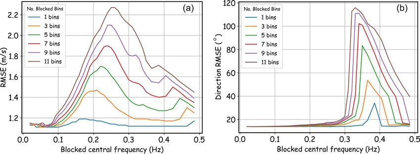
4                                                         H. Jiang: Wind speed and direction estimation from wave spectra

wind speed, the DNN can give an estimation with an overall        For U10 > 20 m s−1 , the bias becomes higher than the SD,
RMSE of ∼ 1.3 m s−1 and a small overall bias. For wind di-        which means the systematic error becomes the main contrib-
rection, the RMSE is ∼ 16◦ for U10 > 7 m s−1 . These results      utor to the RMSE. This is not surprising because the air–sea
show significant improvement compared to the error metrics        interaction becomes much more complicated during extreme
of Voermans et al. (2020).                                        wind, and it is also noted that the U10 extrapolated from
    It is noted that the sampling duration is ∼ 20 min for wave   the wind speed measured at 4–5 m might be overestimated
measurements and ∼ 10 min for wind measurement. Differ-           to some extent in extreme sea states because the anemome-
ently from the capillary waves with very high frequencies         ters might be within the wave boundary layer (Babanin et al.,
always in instant equilibrium with the local wind, the growth     2018). The overall RMSEs of U10 retrieved from spaceborne
of gravity waves is time-dependent. Besides the current wind      altimeters and scatterometers using corresponding state-of-
information, the wave spectrum measured by a buoy at a            the-art combinations of sensors and algorithms are ∼ 1.2 and
given location and time also contains remote and past wind        ∼ 1.0 m s−1 , respectively, compared to buoy measurements
information (Jiang and Mu 2019) because the wave spectrum         (Jiang et al., 2020; Wang et al., 2021). According to the
is, to some degree, integrated winds. Therefore, it is possi-     RMSE, the accuracy of the DNN-estimated U10 is higher
ble that the buoy wave spectrum can better represent the lo-      than altimeter U10 retrievals, and it is similar to scatterom-
cal wind information some time ago. Based on this idea, the       eter U10 retrievals if the data of U10 < 2 m s−1 are excluded.
wave spectra were also collocated with past wind measure-            For wind directions, the RMSE is larger than 25◦ when
ments using different time lags. For the collocations of each     U10 < 5 m s−1 but decreases fast with the increase in U10 .
time lag, DNNs were re-trained to estimate the correspond-        The RMSE becomes less than 20, 15, and 13◦ for U10 val-
ing wind speed and directions and the error metrics were re-      ues of 6, 8, 10 m s−1 , respectively. Beyond U10 = 10 m s−1 ,
computed. The error metrics as a function of time lag are         the RMSE of DNN-estimated wind directions slightly in-
shown in Fig. 3. The results indicate that the DNN performs       creases with the increase in U10 but remains < 20◦ until
significantly better in estimating wind information from a        U10 > 21 m s−1 . It is noted that there were less than 100
short period ago than the current wind information. The best      samples for U10 > 21 m s−1 , and most of them correspond to
error metrics for wind speed and wind direction were found        some strong cyclones where the directions of the wind vary
at 40–50 and 40–60 min before the end of wave sampling            rapidly. Following Voermans et al. (2020), if only the con-
time, respectively. Voermans et al. (2020) found that the wind    dition of U10 > 7 m s−1 was considered, the overall RMSE
acceleration is related to model error residuals, which is con-   of the DNN-estimated wind directions was only ∼ 14◦ . To
sistent with the results here.                                    test the robustness of the DNN framework, we tried the ran-
    Obtaining wind information with only a 40 min delay (near     dom division, training, and validation processes more than 20
real time) is acceptable for most scientific and operational      times, and the resulting error metrics in the validation data
applications. Therefore, the DNNs for wind of a 40 min de-        set stayed stable, meaning that there was no change in the
lay were used in the following analysis. The results of wind      first two significant digits of RMSEs of both U10 (1.1 m s−1 )
speed and direction in the validation data set are shown in       and wind directions (14◦ ). Wind direction information is also
Fig. 2b and e, respectively. The corresponding error metrics      available from spaceborne scatterometers, and the RMSE of
as a function of directly measured U10 are shown in Fig. 2c       wind directions between scatterometers (e.g., ASCAT-B and
and 2f. The overall RMSE for U10 is ∼ 1.1 m s−1 and is only       ASCAT-C, OSCAT2, HSCAT-B) and buoys is 15–18◦ ac-
∼ 1 m s−1 for U10 between 2 and 10 m s−1 , where the sample       cording to Wang et al. (2021). Therefore, the performance
size is relatively large. The DNN model tends to overestimate     of the DNN model is also as good as state-of-the-art scat-
the U10 when it is lower than 2 m s−1 , and the DNN model         terometers with respect to wind directions for U10 > 7 m s−1 .
seldom gives an output of U10 of less than 1 m s−1 . These are       The error metrics of the DNN-estimated wind information
probably because the NDBC buoys do not respond well to            (with a time lag of 40 min) for different buoy locations are
the small waves generated by very low wind while the geo-         shown in Fig. 1. The error metrics vary with buoy locations.
physical noises such as ocean currents have a large impact        The distribution of U10 RMSE for individual buoys is similar
on the wind estimation during low wind speed. Meanwhile,          to that of Voermans et al. (2020), but the RMSE values are
it is noted that other indirect methods for wind speed estima-    much lower here. For most buoys in the open oceans to the
tion, such as remote sensing, also always overestimate low        south of 40◦ N, the RMSEs of DNN-estimated U10 and wind
wind speed (e.g., Stopa et al., 2017; Jiang et al., 2020). Both   directions (for U10 > 7 m s−1 ) are less than 1.0 m s−1 and
the bias and SD increase with the U10 when U10 > 10 m s−1 .       10◦ , respectively. Two buoys are found to have a U10 RMSE
This is partly because the distribution of wind speed is not      larger than 2 m s−1 : Station 44066 (2.1 m s−1 ) at ∼ 40◦ N
uniform and the error in DNN is often larger for the less         on the US East Coast and Station 46070 (2.2 m s−1 ) in the
sampled conditions. Although the DNN model tends to un-           southwest Bering Sea. It is noted that the biases of U10 for
derestimate high wind speed, the relative RMSE remains less       the two buoys (44066 and 46070) are also large. After a
than 14 % for U10 < 20 m s−1 and the accuracy is also im-         further check of the time series of measured and estimated
proved for high U10 compared to Voermans et al. (2020).           U10 , it is found that there seems to be an anemometer prob-

Atmos. Meas. Tech., 15, 1–9, 2022                                                     https://doi.org/10.5194/amt-15-1-2022
H. Jiang: Wind speed and direction estimation from wave spectra 5 Figure 2. (a–c) Comparison between wind speeds measured by buoys and those estimated by wave spectra. (a) Scatterplot of collocated DNN-estimated wind speed and directly measured wind speed. (b) The same as (a), but the spectra were used to estimate the wind speed 40 min previously. (c) The bias, SD, and RMSE of the DNN-estimated wind speed 1 h previously as a function of directly measured wind speed. The blue shading indicates the empirical distribution function of directly measured wind speed. (d–f) The same as (a–c) but for wind directions. Figure 3. (a) The RMSE and CC of the DNN-estimated wind speed as a function of lag time between wave and wind measurements (waves’ end sampling time minus winds’ end sampling time). (b) The RMSE of DNN-estimated wind direction as a function of lag time between wave and wind measurements for wind speed higher than 7 m s−1 . lem at Station 44066 from 22 January to 13 February 2014 estimation or overestimation of U10 for a long period has to (Fig. 4a). The measured and estimated U10 values have a be attributed to the problem of either wind or wave sensor. good agreement before 22 January 2014, but the measured Therefore, such a DNN-based U10 estimation model can also U10 values become significantly lower than the estimated serve as an additional quality control/monitoring method for ones after 22 January 2014. After a sudden drop on 26 Jan- wind and wave sensors on meteorological buoys. If the bias uary 2014, the measured U10 remains lower than 5 m s−1 between estimated and measured U10 remains significant for for more than 15 d, which is unrealistic. A similar condition a short period (e.g., 3–5 d), the wind and wave data then happened at Station 46070 from 3 March to 20 April 2016 need to be further checked or discarded. Because the buoy (Fig. 4b), when the estimated U10 suddenly becomes signifi- data have been quality controlled by NDBC, such conditions cantly lower than the measured U10 . Because the DNN model were only identified in the two cases in Fig. 4. If we remove is unbiased and time-independent, such a systematic under- the bad-quality data in Fig. 4, the U10 RMSEs for Station https://doi.org/10.5194/amt-15-1-2022 Atmos. Meas. Tech., 15, 1–9, 2022
6                                                          H. Jiang: Wind speed and direction estimation from wave spectra

44066 and 46070 will drop to only 1.10 and 1.25 m s−1 , re-        selves like with the condition shown in Fig. 4. Similar condi-
spectively.                                                        tions occur at some other buoys with RMSEs > 20◦ (46001
    The other two buoys with relatively high U10 RMSEs             and 44009). Two aforementioned buoys, 46087 and 46088,
(> 1.5 m s−1 ), Station 46087 and 46088, are both at the Strait    that are impacted by currents also have RMSEs > 20◦ . The
of Juan de Fuca where tidal currents are strong. First of all,     reason for RMSE > 20◦ is unknown for the other two buoys,
the wind estimated from wave measurements is the wind rel-         but errors of ∼ 180◦ sometimes occur at the two buoys, sig-
ative to currents because waves are forced by relative wind. A     nificantly increasing the overall RMSE.
strong current will make the estimated relative wind deviate
from the absolute wind from the anemometer, introducing er-
rors into the DNN model. Secondly, the phase velocity of the       4   Discussions
high-frequency waves and the current velocity are at the same
order of magnitude during strong currents. In this case, the       The wind information estimated from wave spectra achieves
dispersion relation of high-frequency waves is strongly dis-       good accuracy, but the DNN model uses all available wave
torted by the currents via Doppler shift. This will lead to dif-   spectral information as the input. Usually, not all input terms
ferent frequency spectra for the same wavenumber spectra,          are important for the model. Therefore, we tried to refine the
introducing another error source for DNN-estimated wind            DNN model using a sensitivity test. By blocking some of the
speed. The surface currents are generally larger in coastal re-    inputs (setting the values of normalized input to zeros), one
gions (tides) and westerlies (wind drifts) than in low-latitude    can know which input is more important for the DNN model.
open oceans, which can explain the spatial distributions of           Low-frequency waves are usually not coupled to the local
the U10 RMSE and can also partly explain why this model            wind; thus, the importance of different frequency bins was
tends to underestimate large winds. Strong drifts along the        analyzed. The RMSEs after blocking some frequencies are
wind direction will shift the wind-wave energy to lower fre-       shown in Fig. 5. For U10 , it can be seen that inputs under
quencies.                                                          0.1 Hz are not important for the model, and blocking only
    If the aforementioned problematic data are excluded from       one frequency bin has little impact on the result. However,
the training and validation data set (they are included in the     blocking more bins at high frequencies, especially the bins
results in Figs. 1–4), the overall performance of the model        near 0.2 Hz, has large impacts. For wind directions, it seems
will not be significantly improved (the overall RMSE will be       the inputs under 0.25 Hz are not important and the inputs near
reduced by only 0.02 m s−1 ) because the number of samples         0.38 Hz play the most important role in the model. Therefore,
for these corrupt data is very small compared to the over-         what the DNN learns from the data is a weighting average
all sample size. However, the U10 RMSEs will be less than          of the information from different frequencies. Voermans et
1.5 m s−1 for all buoys at different locations. This indicates     al. (2020) also only considered the wave spectra higher than
that the geographic dependence of the DNN model’s error is         some frequencies in a spectrum, which is consistent with the
weak. To further test the robustness of the DNN model in dif-      model here.
ferent locations, the training set, and validation set were di-       The importance of each of the Fourier coefficients was
vided according to the buoys’ locations. The data from buoys       also analyzed. For the U10 (wind direction) DNN, the RM-
45001–51101 (53 buoys) were selected as the training set and       SEs after blocking E, α1 , α2 , r1 , and r2 are 3.75, 1.17, 1.14,
the buoys 41002–44066 (48 buoys) were selected as the val-         1.47, and 1.20 m s−1 (17.3, 111.9, 16.2, 14.3, and 14.4◦ , for
idation set. The locations, wind-wave climate, and other en-       U10 > 7 m s−1 ), respectively. This indicates that E and α1
vironmental properties are significantly different for the two     are the most important parameters for estimating U10 and
sets because none of the buoys in the validation set is in the     wind directions, respectively. This is in line with Voermans
same basin as the buoys in the training set. In this case, the     et al. (2020), where E and α1 are the only parameters for the
established DNN model still has a good performance in the          estimation of U10 and wind directions, respectively. Mean-
validation set with an RMSE of ∼ 1.15 m s−1 (the result can        while, r1 (E and α2 ) seems to also play some roles in the esti-
be seen in the reply to the reviewer in the online discussion).    mation of U10 (wind directions). If we re-train the model with
    For wind directions (U10 > 7 m s−1 ), the lowest RMSE is       only E (α1 ), the RMSE in the validation set can only reach
  ◦
7 and 68/94/100 out of the 101 buoys have RMSEs of                 1.26 m s−1 (15.5◦ ), slightly worse than the original model.
less than 14◦ /20◦ /22◦ , showing the robustness of the DNN        This is probably because r1 contains the wave-spreading in-
model. The spatial distribution of RMSE is similar to that of      formation and the wave spreading at high frequencies is also
U10 RMSE (the CC between the RMSEs of U10 and wind                 correlated to the wind speed, which can be used to slightly
directions is 0.51, significant at 99.9 % level) with the low-     reduce the random error in the U10 from E only. Similarly,
est value in the open ocean at low latitudes. The only buoy        α2 information can also partially reveal the wave direction at
with an RMSE larger than 22◦ is at Station 46082 (59.68◦ N,        high frequencies, and E is helpful to give the energy weights
143.37◦ W). However, after a further check of the data, a bias     for each frequency, which in turn are helpful to reduce the
of ∼ 25◦ was found after 22 September 2018 (not shown), in-        random error in estimated wind directions. The above sensi-
dicating there might be something wrong with the data them-        tivity test indicates that E and r1 above 0.1 Hz (α1 , α2 , and E

Atmos. Meas. Tech., 15, 1–9, 2022                                                       https://doi.org/10.5194/amt-15-1-2022
H. Jiang: Wind speed and direction estimation from wave spectra 7
Figure 4. Time-series comparison of directly measured (orange) and DNN-estimate (blue) wind speed for (a) Station 44066 from 16 January
to 15 February 2014 and (b) Station 46070 from 1 February to 20 April 2016. For 44066, the measured wind speed values became significantly
lower than the DNN-estimated ones after 22 January 2014. For 46070, the DNN-estimated wind speed values became significantly lower
than the directly measured ones after 3 March 2016. The date is given in the format year–month–day.
Figure 5. (a) The RMSE between DNN-estimated and directly measured U10 as a function of the blocked central frequency. Different
colors indicate the results of blocking different numbers of bins. For example, the orange line indicates that the RMSE of the DNN model is
∼ 1.45 m s−1 (the peak) when the input at 0.2 Hz and its two neighboring bins, 0.19 and 0.21 Hz, are blocked (set to zero after normalization).
(b) is the same as (a) but for the RMSE of wind direction.
above 0.25 Hz) are the most important inputs for the estima- wind directions) without changing other settings, the perfor-
tion of U10 (wind directions), which is also in line with Vo- mance of the models is nearly the same as the original ones.
ermans et al. (2020). Previous studies of wind remote sens- The RMSEs remain less than 1.15 m s−1 and 14.5◦ for U10
ing showed that the modulation of swells on capillary waves and wind directions, respectively, in 20 independent experi-
has some impacts on the wind speed retrievals (e.g., Stopa et ments.
al., 2017; Li et al., 2018; Jiang et al., 2020). Long swells also
modulate short wind seas (waves with relatively high fre-
quencies measured by buoys; they are gravity waves instead
of capillary waves). If this modulation process significantly 5 Concluding remarks
impacts the buoy wind-estimation model, removing the long-
swell information will negatively impact the model accuracy. Ocean wave spectra can be used to estimate sea surface
However, according to the results in Fig. 5, the swell’s modu- winds. Here, we trained two DNNs that can estimate U10 and
lation on wind seas has little impact on wind estimation using wind directions ∼ 40 min previously from high-frequency
buoy wave spectra. If we re-train a DNN using only these in- wave spectra. The overall accuracy of the wind-estimation
puts (33 × 2 = 66 inputs for U10 , and 17 × 3 = 51 inputs for DNN models is comparable with the state-of-the-art scat-
terometers under moderate U10 . The two models can also be
https://doi.org/10.5194/amt-15-1-2022 Atmos. Meas. Tech., 15, 1–9, 20228 H. Jiang: Wind speed and direction estimation from wave spectra
used as a quality control tool for wind and wave measure- Supplement. The supplement related to this article is available on-
ments from meteorological buoys. line at: https://doi.org/10.5194/amt-15-1-2022-supplement.
The DNNs were trained using a large number of data from
only NDBC buoys and not compact wave buoys. However,
applying the two models directly to compact wave buoy data Competing interests. The contact author has declared that there are
(after interpolating the spectra from compact buoys into the no competing interests.
frequency bins of NDBC buoys) will not result in signifi-
cantly lower accuracy. This is because the DNN will auto-
matically select the NDBC wave spectra in the frequency Disclaimer. Publisher’s note: Copernicus Publications remains
neutral with regard to jurisdictional claims in published maps and
with relatively high accuracy, and the accuracy of measured
institutional affiliations.
spectra from compact wave buoys is usually higher.
For the wave data from NDBC buoys, the performance of
the U10 DNN is significantly biased when U10 is too high or Financial support. This research has been supported by the Key
too low, and the performance of the wind direction DNN be- Special Project for Introduced Talents Team of the Southern Ma-
comes worse with the decrease in U10 . Also, the accuracy of rine Science and Engineering Guangdong Laboratory (Guangzhou)
both models decreases when the surface currents are strong. (grant no. GML2019ZD0604), the National Natural Science Foun-
We believe these shortcomings can be partly solved by com- dation of China (grant nos. U2006210, 41806010), and the Key
pact wave drifters, resulting in better accuracy in estimating Research and Development Program of Hubei Province (grant no.
near-real-time wind properties. First, a smaller buoy size can 2020BCA080).
resolve high-frequency wave spectra more accurately, which
is helpful for wind estimation. Second, in the condition of
strong wind or currents, the moving velocity of the wave Review statement. This paper was edited by Ad Stoffelen and re-
drifter is usually similar to that of the surface current, mak- viewed by three anonymous referees.
ing the wavenumber and frequency spectra follow a disper-
sion relation again in the buoy reference system. This can
compensate for some of the errors induced by strong surface
currents or wind-induced drifts. Therefore, significantly bet-
References
ter accuracy can be achieved by training new DNN models
with the spectral data (maybe also the drifting velocity data) Babanin, A. V., McConochie, J., and Chalikov, D.: Winds near
from compact buoys using collocated wind and wave mea- the surface of waves: Observations and modeling. J. Phys.
surements. Such measurements can be obtained by placing Oceanogr., 48, 1079–1088, https://doi.org/10.1175/JPO-D-17-
some compact buoys near meteorological buoys or simply 0009.1, 2018.
using the scatterometer or re-analysis wind as the training Hsu, S. A., Meindl, E. A., and Gilhousen, D. B.: De-
target. termining the power-law wind-profile exponent un-
Finally, we hope to point out that such DNN models need der near-neutral stability conditions at sea, J. Appl.
not be trained from the beginning using a large number of Meteorol., 33, 757–765, https://doi.org/10.1175/1520-
data. The DNN models presented in this paper can serve as 0450(1994)0332.0.CO;2 1994.
Jiang, H.: Indirect validation of ocean remote sensing data via nu-
pre-trained models which will significantly reduce the com-
merical model: An example of wave heights from altimeter, Re-
plexity of training the new models. With the compact wave
mote Sens., 13, 2627, https://doi.org/10.3390/rs12162627, 2020.
buoys becoming increasingly widely used in observing wave Jiang, H. and Mu, L.: Wave Climate from Spectra and Its Connec-
parameters, their global network can be a new good-quality tions with Local and Remote Wind Climate, J. Phys. Oceanogr.,
data source for both waves and wind after applying these 49, 543–559, 2019.
models. Jiang, H., Babanin, A. V., and Chen, G.: Event-based valida-
tion of swell arrival time, J. Phys. Oceanogr., 46, 3563–3569,
https://doi.org/10.1175/JPO-D-16-0208.1, 2016.
Code and data availability. The NDBC data are available from Jiang, H., Zheng, H., and Mu, L.: Improving Altime-
the website of the National Centers for Environmental Information ter Wind Speed Retrievals Using Ocean Wave Pa-
(2021, https://www.ncei.noaa.gov/data/oceans/ndbc/cmanwx/). rameters, IEEE J. Sel. Top. Appl., 13, 1917–1924,
The two established wind-estimation DNN models are available https://doi.org/10.1109/JSTARS.2020.2993559, 2020.
as Python .plk files in the Supplement where the corresponding Li, H., Mouch, A., and Stopa, J. E.: Impact of Sea
examples (as Python code) of implementing the two models are State on Wind Retrieval from Sentinel-1 Wave
also available. Mode Data, IEEE J. Sel. Top. Appl., 12, 559–566,
https://doi.org/10.1109/JSTARS.2019.2893890, 2018.
National Centers for Environmental Information: https://www.ncei.
noaa.gov/data/oceans/ndbc/cmanwx/, last access: 22 December
2021.
Atmos. Meas. Tech., 15, 1–9, 2022 https://doi.org/10.5194/amt-15-1-2022H. Jiang: Wind speed and direction estimation from wave spectra 9 Smit, P. B., Houghton, I. A., Jordanova, K., Portwood, Wang, J. K., Aouf, L., Dalphinet, A., Zhang, Y. G., Xu, T., Shapiro, E., Clark, D., Sosa, M., and Janssen, T. Y., Hauser, D., and Liu, J. Q.: The wide swath signifi- T.: Assimilation of significant wave height from dis- cant wave height: An innovative reconstruction of significant tributed ocean wave sensors, Ocean Model., 159, 101738, wave heights from CFOSAT’s SWIM and scatterometer us- https://doi.org/10.1016/j.ocemod.2020.101738, 2021. ing deep learning, Geophys. Res. Lett., 48, e2020GL091276, Steele, K. E., Wang, D. W., Earle, M. D., Michelena, E. D., and https://doi.org/10.1029/2020GL091276, 2021. Dagnall, R. J.: Buoy pitch and roll computed using three angular Wang, Z., Zou, J., Stoffelen A., Lin, W., Verhoef, A., Li, X., He, Y., rate sensor, Coast. Eng., 35, 123–139, 1998. Zhang, Y., and Lin, M.: Scatterometer Sea Surface Wind Product Stopa, J. E., Mouche, A., Chapron, B., and Collard, F.: Validation for HY-2C, IEEE J. Sel. Top. Appl., 14, 6156–6164, Sea state impacts on wind speed retrievals from C- https://doi.org/10.1109/TGRS.2019.2963690, 2021. band radars, IEEE J. Sel. Top. Appl., 10, 2147–2155, Young, I. R., Verhagen, L. A., and Banner, M. L.: A note on the bi- https://doi.org/10.1109/JSTARS.2016.2609101, 2017. modal directional spreading of fetch-limited wind waves, J. Geo- Voermans J. J., Smit, P. B., Janssen, T., and Babanin, A. phys. Res., 100, 773–778, https://doi.org/10.1029/94JC02218, V.: Estimating wind speed and direction using wave 1995. spectra, J. Geophys. Res.-Oceans, 125, 2019JC015717, https://doi.org/10.1029/2019JC015717, 2020. https://doi.org/10.5194/amt-15-1-2022 Atmos. Meas. Tech., 15, 1–9, 2022
You can also read