Wire Detection, Reconstruction, and Avoidance for Unmanned Aerial Vehicles
←
→
Page content transcription
If your browser does not render page correctly, please read the page content below
Wire Detection, Reconstruction, and
Avoidance for Unmanned Aerial Vehicles
                   Ratnesh Madaan
                   CMU-RI-TR-18-61
                      August 2018

               School of Computer Science
               Carnegie Mellon University
                  Pittsburgh, PA 15213
                  Thesis Committee:
                 Sebastian Scherer, Chair
                      Michael Kaess
                     Sankalp Arora

    Submitted in partial fulfillment of the requirements
     for the degree of Master of Science in Robotics.

            Copyright c 2018 Ratnesh Madaan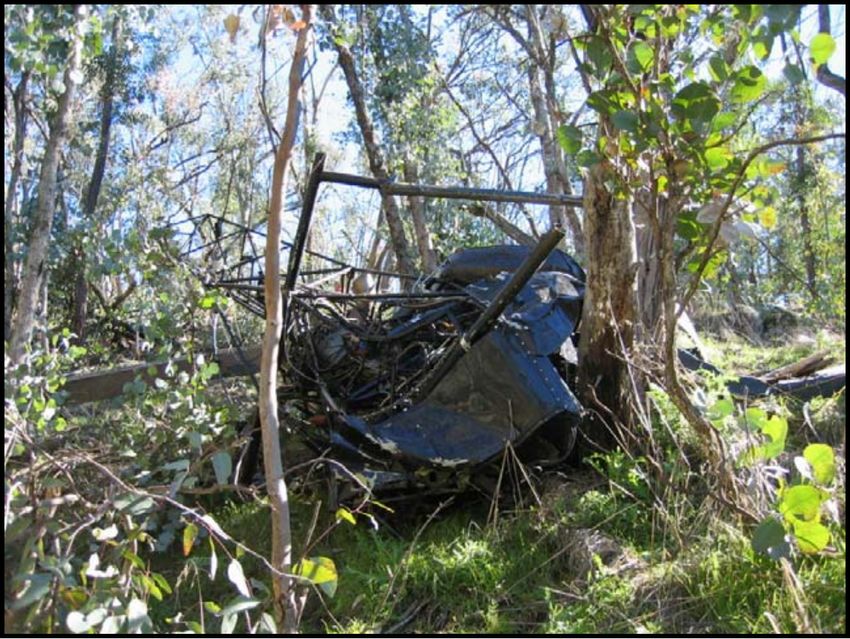
Abstract
    Thin objects, such as wires and power lines are one of the most challenging
obstacles to detect and avoid for UAVs, and are a cause of numerous accidents
each year. This thesis makes contributions in three areas of this domain: wire
segmentation, reconstruction, and avoidance.
    Pixelwise wire detection can be framed as a binary semantic segmentation
task. Due to the lack of a labeled dataset for this task, we generate one by
rendering photorealistic wires from synthetic models and compositing them into
frames from publicly available flight videos. We show that dilated convolutional
networks trained on this synthetic dataset in conjunction with a few real images
perform with reasonable accuracy and speed on real-world data on a portable
GPU.
    Given the pixel-wise segmentations, we develop a method for 3D wire recon-
struction. Our method is a model-based multi-view algorithm, which employs
a minimal parameterization of wires as catenary curves. We propose a bundle
adjustment-style framework to recover the model parameters using non-linear
least squares optimization, while obviating the need to find pixel correspon-
dences by using the distance transform as our loss function. In addition, we
propose a model-free voxel grid method to reconstruct wires via a pose graph
of disparity images, and briefly discuss the pros and cons of each method.
    To close the sensing-planning loop for wire avoidance, we demonstrate a
reactive, trajectory library-based planner coupled with our model-free recon-
struction method in experiments with a real UAV.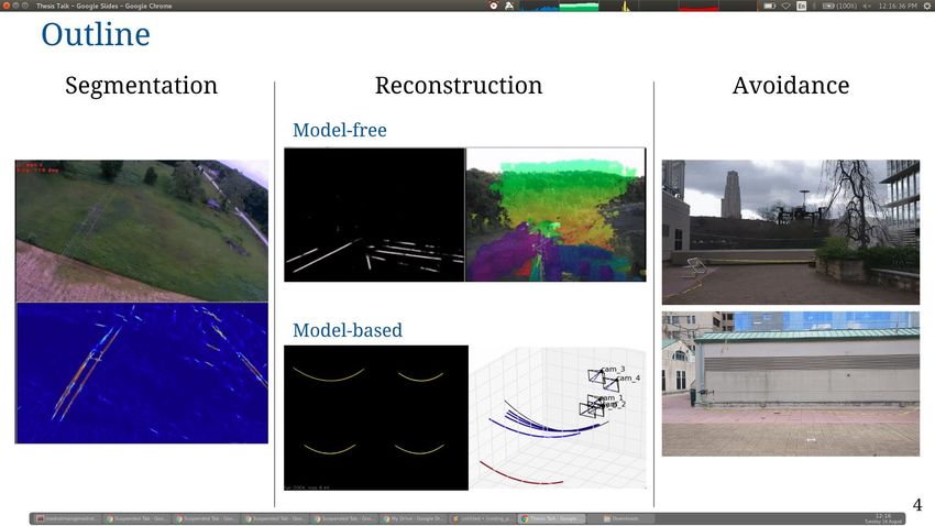
iv
Acknowledgments
    I would like to begin by thanking my advisor, Basti, for giving me an oppor-
tunity to work on an important and interesting problem. Thanks for allowing
to me to explore new ideas, while always ensuring I am always on track for
my thesis. A big thanks goes out to Daniel Maturana, Geetesh Dubey, and
Michael Kaess, for their critical technical contributions, feedback, and advice
in the relevant chapters. I am grateful for Michael for the frequent meetings
during the last semester here, I’ll miss them. Also thanks to Sankalp Arora
and Sanjiban Choudhury, for helpful advice and feedback during my time here.
Thanks again to Daniel and Geetesh for the same.
    Thanks to John Keller, Silvio Maeta, and Greg Armstrong for building the
systems and help with experimentation over the two years. Thanks to Jaskaran
Singh Grover for jumping in for a critical review of this thesis a night before
its due. Thanks to Eric Westman for reviewing my approach now and then.
Thanks to Nora Kazour, Rachel Burcin, and Sanae Minick for bringing me
to CMU multiple times. Thanks to Robbie Paolini, Erol Sahin, Matt Mason,
and Rachel again for bringing me to CMU via RISS 2015, and great mentorship
over the summer. Thanks to my friends Tanmay Shankar and Sam Zeng for life
outside work. Thanks Rohit Garg for the expensive coffee grabs and awesome
conversation. Thanks Rogerio Bonatti for all things McKinsey.
    We gratefully acknowledge Autel Robotics for supporting this work, under
award number A018532.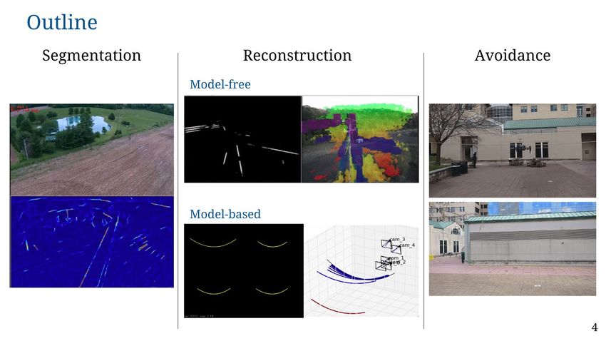
vi
Contents
1 Introduction 1
1.1 Motivation . . . . . . . . . . . . . . . . . . . . . . . . . . . . . . . . . . . . 1
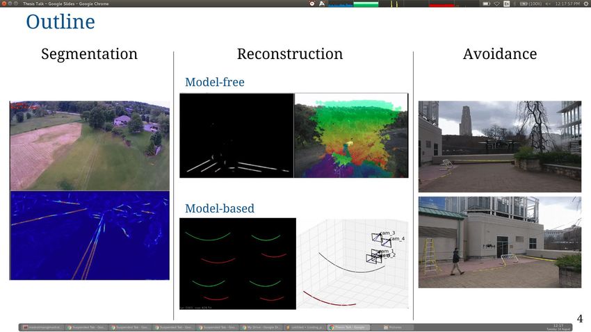
1.2 Thesis Overview . . . . . . . . . . . . . . . . . . . . . . . . . . . . . . . . . 4
2 Wire Segmentation from Monocular Images 7
2.1 Introduction . . . . . . . . . . . . . . . . . . . . . . . . . . . . . . . . . . . 7
2.2 Related Work . . . . . . . . . . . . . . . . . . . . . . . . . . . . . . . . . . 9
2.2.1 Wire detection using traditional computer vision . . . . . . . . . . . 9
2.2.2 Semantic segmentation and edge detection using deep learning . . . 10
2.3 Approach . . . . . . . . . . . . . . . . . . . . . . . . . . . . . . . . . . . . 12
2.3.1 The search for the right architecture . . . . . . . . . . . . . . . . . 12
2.3.2 Generating synthetic data . . . . . . . . . . . . . . . . . . . . . . . 13
2.3.3 Class Balancing Loss Function . . . . . . . . . . . . . . . . . . . . . 13
2.3.4 Explicitly providing local evidence of wires . . . . . . . . . . . . . . 13
2.4 Experiments and Results . . . . . . . . . . . . . . . . . . . . . . . . . . . . 13
2.4.1 Evaluation Metrics . . . . . . . . . . . . . . . . . . . . . . . . . . . 13
2.4.2 Grid Search . . . . . . . . . . . . . . . . . . . . . . . . . . . . . . . 14
2.4.3 Baselines . . . . . . . . . . . . . . . . . . . . . . . . . . . . . . . . . 15
2.5 Conclusion and Future Work . . . . . . . . . . . . . . . . . . . . . . . . . . 17
3 Multi-view Reconstruction of Wires using a Catenary Model 23
3.1 Introduction . . . . . . . . . . . . . . . . . . . . . . . . . . . . . . . . . . . 23
3.2 Related Work . . . . . . . . . . . . . . . . . . . . . . . . . . . . . . . . . . 24
3.3 Approach . . . . . . . . . . . . . . . . . . . . . . . . . . . . . . . . . . . . 25
3.3.1 Catenary Model . . . . . . . . . . . . . . . . . . . . . . . . . . . . . 25
3.3.2 Objective Function . . . . . . . . . . . . . . . . . . . . . . . . . . . 27
3.3.3 Optimization Problem . . . . . . . . . . . . . . . . . . . . . . . . . 28
3.4 Experiments and Results . . . . . . . . . . . . . . . . . . . . . . . . . . . . 29
3.4.1 Simulation . . . . . . . . . . . . . . . . . . . . . . . . . . . . . . . . 29
3.4.2 Real Data . . . . . . . . . . . . . . . . . . . . . . . . . . . . . . . . 30
3.5 Analytical Jacobian Derivation . . . . . . . . . . . . . . . . . . . . . . . . 33
3.6 Conclusion . . . . . . . . . . . . . . . . . . . . . . . . . . . . . . . . . . . . 41
3.7 Future Work . . . . . . . . . . . . . . . . . . . . . . . . . . . . . . . . . . . 41
3.7.1 Computing the width of the catenary . . . . . . . . . . . . . . . . . 41
vii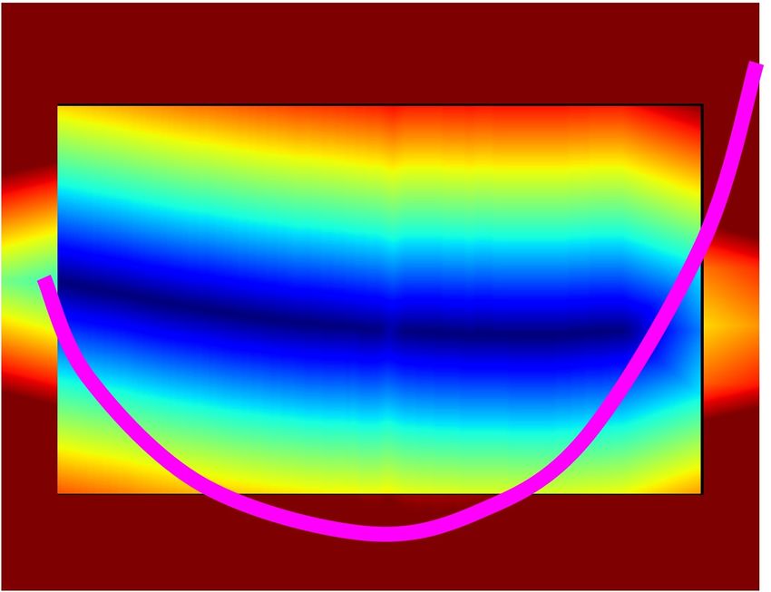
3.7.2   Closing the loop by modeling uncertainty . . . . . . . . . . . . . . .                         42
         3.7.3   Handling multiple wires . . . . . . . . . . . . . . . . . . . . . . . .                        44

4 Model-free Mapping and Reactive Avoidance                                                                     47
  4.1 Acknowledgements . . . . . . . . . . . . . . . . . . . . .        .   .   .   .   .   .   .   .   .   .   47
  4.2 Introduction . . . . . . . . . . . . . . . . . . . . . . . . .    .   .   .   .   .   .   .   .   .   .   47
  4.3 Related Work . . . . . . . . . . . . . . . . . . . . . . . .      .   .   .   .   .   .   .   .   .   .   48
      4.3.1 Depth or Disparity map based Obstacle Detection             .   .   .   .   .   .   .   .   .   .   48
  4.4 Approach . . . . . . . . . . . . . . . . . . . . . . . . . .      .   .   .   .   .   .   .   .   .   .   49
      4.4.1 Monocular Wire Detection . . . . . . . . . . . . .          .   .   .   .   .   .   .   .   .   .   49
      4.4.2 Characterizing Disparity Space Uncertainty . . .            .   .   .   .   .   .   .   .   .   .   50
      4.4.3 Configuration-Space Expansion in Disparity Space            .   .   .   .   .   .   .   .   .   .   51
      4.4.4 Probabalistic Occupancy Inference . . . . . . . .           .   .   .   .   .   .   .   .   .   .   55
      4.4.5 Collision Checking . . . . . . . . . . . . . . . . .        .   .   .   .   .   .   .   .   .   .   56
      4.4.6 Pose Graph of Disparity Images . . . . . . . . . .          .   .   .   .   .   .   .   .   .   .   57
  4.5 Planning & Motion Control . . . . . . . . . . . . . . . .         .   .   .   .   .   .   .   .   .   .   57
  4.6 System and Experiments . . . . . . . . . . . . . . . . . .        .   .   .   .   .   .   .   .   .   .   58
      4.6.1 System . . . . . . . . . . . . . . . . . . . . . . . .      .   .   .   .   .   .   .   .   .   .   58
      4.6.2 Experiments . . . . . . . . . . . . . . . . . . . . .       .   .   .   .   .   .   .   .   .   .   60
  4.7 Results . . . . . . . . . . . . . . . . . . . . . . . . . . . .   .   .   .   .   .   .   .   .   .   .   61
      4.7.1 Simulation Results . . . . . . . . . . . . . . . . .        .   .   .   .   .   .   .   .   .   .   61
      4.7.2 Wire Avoidance Results . . . . . . . . . . . . . .          .   .   .   .   .   .   .   .   .   .   62
      4.7.3 Disparity Map based Obstacle Avoidance Results              .   .   .   .   .   .   .   .   .   .   62
  4.8 Conclusion and Future Work . . . . . . . . . . . . . . . .        .   .   .   .   .   .   .   .   .   .   63

5 Conclusion                                                                                                    65
  5.1 Associated Publications . . . . . . . . . . . . . . . . . . . . . . . . . . . .                           65

Bibliography                                                                                                    67

                                             viii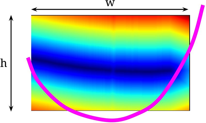
List of Figures
1.1 Bell 206B helicopter after striking powerlines during locust control cam-
paigns at different locations and date. Image from Australian Transport
Safety Bureau [2006]. . . . . . . . . . . . . . . . . . . . . . . . . . . . . . . 3
1.2 Bell 47G-3B-1 Soloy helicopter after striking powerlines near Wodonga on
19 June 2004. Image from Australian Transport Safety Bureau [2006]. . . . 3
1.3 Thesis outline . . . . . . . . . . . . . . . . . . . . . . . . . . . . . . . . . . 4
2.1 A few samples from our synthetically generated dataset along with ground
truth labels of wires. Video examples available at this link and our project
page. . . . . . . . . . . . . . . . . . . . . . . . . . . . . . . . . . . . . . . 8
2.2 Close up of synthetic wires rendered using POV-Ray [POV-Ray, 2004]. . . 9
2.3 Precision recall curves obtained by evaluating our models on USF test split
with RGB input, after finetuning our models on USF train split after pre-
training on synthetid data. Each subfigure has the same front end module,
while the context module changes as shown in the legends. Numbers in
paranthesis are the Average Precision scores for the respective model. In all
cases we can see that adding increasing dilation increases the precision of
the classifier at various recall levels (except for one case in k32-k32-k32-k32-
k32-k32’s series where the model with the maximum dilation didn’t converge. 19
2.4 Precision Recall curves of the top models from our grid search experiment
(in bold text in Table 2.3). Legend shows Average Precision scores on the
USF test split, and speed on the NVIDIA TX2 in frames per second. . . . 20
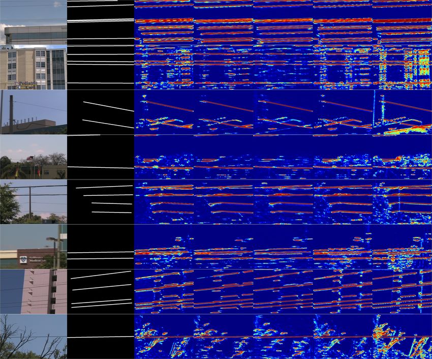
2.5 Qualitative results on real images with model k32-k32-k32-k32-d1-d2-d4-d8-
d16-d1-k2 trained on our synthetic dataset with input resolution of 720x1280.
High resolution helps the network pick far off (Image 6), very thin wires
(Images 3 and 4), those in clutter (Image 11) and taken when in high speed
(Images 5 and 7). Video available at this link and our project page. . . . . 21
2.6 Qualitative results of our top 5 models after finetuning on the USF dataset
with RGB input. Left to right : Input image, Ground Truth, predictions
with architecture k64-k64-p2-k128-k128-d1-d2-d4-d1-k2, k32-k32-k32-k32-
d1-d2-d4-d8-d16-d1-k2, k32-k32-d1-d2-d4-d8-d16-d1-k2, k32-k32-k32-k32-k32-
k32-d1-d2-d4-d8-d1-k2, k32-k32-k32-k32-k32-k32-d1-d2-d4-d1-k2. . . . . . 22
ix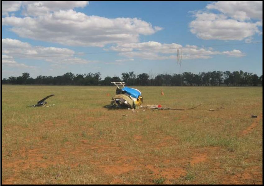
3.1 Schematic of the problem formulation. We are given N binary images
of wire segmentations (red), along with their corresponding camera poses
{C1 , C2 , ..., Cn }. The multiple curves and the transform are indicate various
possible hypotheses. The blue curves denote the projection of the current
hypothesis in each keyframe. . . . . . . . . . . . . . . . . . . . . . . . . . . 24
3.2 (a) Catenary curves from Equation 3.1 in the local catenary frame, Fcat with
varying sag parameter (a) values. (b) Our 3D catenary model is obtained by
defining the local catenary frame, Fcat with respect to a world frame, FW .
Note that because the curve is planar and sags under the effect of gravity, we
only need to define a relative yaw instead of a full rotation transform. The
catenary parameters are then given by {xv , yv , zv , ψ, a}. Here, {xv , yv , zv }
are the coordinates of the lowermost of the curve which we also refer to as
the vertex of the catenary, ψ refers to the relative yaw of Fcat w.r.t. FW . . 26
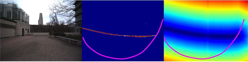
3.3 Example demonstrating our objective function for valid projections of the
catenary hypothesis. Left: RGB image with thin wire running across the
image. This image was taken in the patio behind Newell Simon Hall at
CMU. Middle: Confidence map of per-pixel wire segmentation from our
CNN. Colormap used is Jet. Given this confidence map, the goal is to
establish the distance from the projection of a catenary hypothesis (shown
in pink). Right: We binarize the segmentation map, and use the distance
transform of the binarized segmentations as our objective function. . . . . 27
3.4 (a) This highlights the issue with invalid projections, falling outside the im-
age coordinates. The question then is, how do we quantify the distance
of such invalid pixels from the segmented wire. (b) If we extrapolate the
loss function from the image center, it becomes discontinuous and non-
differentiable at the boundaries of the image. (c) The fix for this is then
intuitive. By extrapolating from the boundary pixels, we mitigate the prob-
lem. The invalid area outside the image is divided into 8 regions. For any
point pji denoted by the arrow heads, we find the corresponding pixel at the
boundary pbi given by the base of the arrow, and extrapolate the value as
explained in the text. . . . . . . . . . . . . . . . . . . . . . . . . . . . . . . 28
3.5 Chain of transformations and jacobians. . . . . . . . . . . . . . . . . . . . 29
3.6 Simulation of random camera placement scenarios. We encourage the reader
to examine the corresponding animations available at the thesis webpage. . 32
3.7 Simulation of avoidance scenarios. We encourage the reader to examine the
corresponding animations available at the thesis webpage. . . . . . . . . . . 35
3.8 Wire detection in 2 handpicked keyframes of total 16 frames we perform
multiview reconstruction on. We perform wire detection on a 300X400 image
and our CNN runs at greater than 3 Hz on an Nvidia TX-2. . . . . . . . . 36
3.9 Experiments on real data. We extract 16 keyframes looking head on at a wire. 38
3.10 Failure case for an avoidance scenario with two cameras. Notice that even
though the loss is going down, we obtain the wrong result due to degeneracy.
We encourage the reader to examine the corresponding animations available
at the thesis webpage. . . . . . . . . . . . . . . . . . . . . . . . . . . . . . 42
x4.1 Wire Mapping using Monocular Detection and Obstacle Perception using Disparity Ex-
pansion. Obstacles perceived using a stereo-camera are shown in red ellipses, and wire
obstacles detected from monocular camera are shown with yellow ellipses. The bottom
half shows the obstacle grid represented by our pose of graph of disparity images. Wires
are shown as black boxes, and stereo camera perceived obstacles are colored by height. 49
4.2 (a) Disparity and corresponding depth values are shown in blue. A Gaussian pdf centred
around a low disparity value (red on X-axis) maps to a long tail distribution (red on
Y-axis) in the depth space, whereas a Gaussian for larger disparity value maps to less
uncertainty in depth space. This explains how we capture difficult to model distributions
in the depth space with a Gaussian counterpoint in the disparity space. (b) Shows the
pixel-wise area expansion of a point obstacle according to robot size in the image plane. 51
4.3 Disparity expansion shown as point cloud. The pink and red point cloud represent the
foreground and background disparity limits. . . . . . . . . . . . . . . . . . . . . 53
4.4 Synthetic disparity generation and expansion of wire. The frontal and backward image
planes show the thin wire projection along with the result of applied expansion steps. . 53
4.5 (a)-(c) show single observations at different heights using our representation. For each
subfigurem, the bottom row shows the simulated camera RGB observation on the left
(white on gray background), and the binary wire detection post expansion on the bot-
tom right. The top row shows the corresponding assumption derived from the binary
detection: we assume the wire is uniformly distributed between a range of depth (4m to
20m from the camera), as is depicted by the voxels colored by their height. The ground
truth wires are shown as black linear point cloud. (d)-(e) show the oblique and side views
of the result of our fusion and occupancy inference. As can be inferred qualitatively,
our approach is successful in mapping the three wires. Again, in (d)-(e) the voxels are
colored by their heights, and the ground truth wires are shown as black lines. The robot
odometry is shown in red, and the individual nodes of the pose-graph are depicted by the
green arrows. . . . . . . . . . . . . . . . . . . . . . . . . . . . . . . . . . . . 54
4.6 Probability mass (shown in blue area) occupied by a robot of radius 0.5m at a distance
of 50m(3.5px) and 5m(35.6px). As the distance increases or disparity decreases the
probability mass occupied by the robot varies. . . . . . . . . . . . . . . . . . . . . 55
4.7 (a) Probability Mass of occupancy, given a robot at disparity d pixels. This curve is used
to compute the log-odds to infer occupancy. (b) Disparity vs Confidence plot obtained
from equation (4.4). This is inexpensive to compute online compared to computation
of probability mass which involves integration of inverse-sensor-model over robot radius.
(c) Occupancy update comparison between log-odds and proposed confidence inference.
Confidence based occupancy update is more conservative in nature and will lead to de-
tection of an obstacle using fewer observations. Hence, this function is pessimistic about
free-space and ensures an obstacle will be detected in all cases when log-odds also detects
an obstacle. . . . . . . . . . . . . . . . . . . . . . . . . . . . . . . . . . . . . 56
4.8 (a) Side view (b) back view of 3D Trajectory Library used on the robot. The Axes
represent the robot pose, red is forward x-axis and blue is down z-axis. . . . . . . . . 58
4.9 Robot-1: Quadrotor platform used for experiments: equipped with stereo camera + color
(middle) camera sensor suite and onboard ARM computer . . . . . . . . . . . . . . 59
xi4.10 System diagram of the robot. Shows the hardware and main software components and
their data exchange. ROS is used to interchange data between various onboard software
components and to provide goal from the ground station. . . . . . . . . . . . . . . 59
4.11 Robot-2: A smaller quadrotor platform used for experiments: equipped with stereo cam-
era sensor suite and onboard ARM computer . . . . . . . . . . . . . . . . . . . . 60
4.12 Demo setup for Robotics Week, 2017 at RI-CMU. The start is on left and the goal is
10 m away on right with several obstacles restricting a direct path, hence forming a
curvy corridor (in blue) to follow. We did more than 100 runs with no failures at 2.5 m/s 61
4.13 This figure shows three timestamps from run 8 of our real world wire avoidance experi-
ment. Top row shows the input color image used for wire detection, disparity map, and
(c-space) expanded wire obstacle map. Bottom row shows corresponding scenarios in
different 3D perspectives (oblique and side). The black voxels are shown for visualization
of wire collision map. (a) Robot observes the wire. (b) Executes upward trajectory. (c)
After ascending upwards enough to avoid the wire, the robot executes a straight trajec-
tory towards a goal 15 m ahead from the start point of the mission. Wire collision map
is updated with new observations void of wire. . . . . . . . . . . . . . . . . . . . . 62
4.14 Time Profile for trajectory library based planner approach on Jetson TX2. . . . . . . 62
xiiList of Tables
2.1 The parameter space over which we perform a grid search. Each context
module from the 2nd column was stacked over each front-end module from
the first column to get a total of 30 models. All layers use 3*3 convolutions.
Each layer is separted by a ‘-’ sign. ‘k’ refers to the number of channels in
each layer. ‘p’ refers to pooling layers, ‘d’ refers to the dilation factor. . . 10
2.2 Results of our grid search experiments. The strings in bold, blue text rep-
resent the front end architecture as explained in text. Each front end is
appended with five different context modules as shown in the Col. 1. We
conduct six experiments, all of which are evaluated on our test split of the
USF dataset. Each experiment category is grouped with the same hue (Col.
2-3, 4-5, 6-7 respectively). Darker color implies better performance. Choice
of colors is arbitrary. Col. 8-11 list the performance speeds on the NVIDIA
TitanX Pascal and the Jetson TX2, with batch size 1 and input resolution
of 480x640. . . . . . . . . . . . . . . . . . . . . . . . . . . . . . . . . . . . 11
2.3 Top models from our grid search. All models were trained on synthetic
data first, then finetuned on our USF dataset test split using RGB input.
Darker color in each colum implies higher accuracy, higher speed (frames
per second) on the TX2, and smaller number of model parameters. Hues
for each column are chosen arbitrarily. . . . . . . . . . . . . . . . . . . . . 16
2.4 Our top models compared with various baselines. The metrics used are Aver-
age Precision(AP), Area under the Curve of ROC diagram(AUC), Optimal
Dataset Scale F1-Score(ODS F-Score) . . . . . . . . . . . . . . . . . . . . . 17
4.1 Occupancy update . . . . . . . . . . . . . . . . . . . . . . . . . . . . . . . . . 56
4.2 Details of our 10 runs of wire avoidance at Gascola, a test site half an hour
away from CMU. Videos available at the thesis webpage. . . . . . . . . . . 63
xiiixiv
Chapter 1

Introduction

1.1     Motivation
We are at an interesting inflection point in the trajectory of Unmanned Aerial Vehicle
(UAV) research and industry. The essential and critical modules - state estimation, con-
trol, and motion planning, have been shown to work reliably in multiple publications and
products. With the fundamentals of autonomous flight figured out, the focus of research
is now shifting to making these algorithms and systems more reliable and robust, and
also on integrating all the components together moving towards higher levels of autonomy.
The industry is developing drone applications for various B2B verticals on platforms by
manufacturers like DJI, and the promise of autonomous drone selfie camera is becoming
a reality [Skydio, 2018]. This also means that the hard problems, the edge cases, which
albeit did receive some amount of attention in the past, are now again being looked closely
upon by both academia and industry. A few examples are :
    • Thin obstacles [Zhou et al., 2017b]
   • Translucent obstacles [Berger et al., 2017, Liu et al., 2017]
   • Unexpected, dynamic obstacles flying towards the UAV [Poiesi and Cavallaro, 2016]
    This thesis addresses an infamous, long-standing problem in the UAV community:
detection, reconstruction and avoidance of wires and power lines, and corresponding ap-
plication areas of automated powerline corridor inspection and management Tuomela and
Brennan [1980a,b], Fontana et al. [1998], Kasturi and Camps [2002], Australian Transport
Safety Bureau [2006], McLaughlin [2006], Rubin and Zank [2007], Yan et al. [2007], Hrabar
[2008], Nagaraj and Chopra [2008], Scherer et al. [2008], Candamo et al. [2009], De Voogt
et al. [2009], Moore and Tedrake [2009], Sanders-Reed et al. [2009], Law et al. [2010], Li
et al. [2010], Jwa and Sohn [2012], Lau [2012], Pagnano et al. [2013], Song and Li [2014],
Pouliot et al. [2015], Ramasamy et al. [2016], Hirons [2017], Flight Safety Australia [2017],
McNally [2018]. Thin wires and similar objects like power lines, cables, ropes and fences
are one of the toughest obstacles to detect for autonomous flying vehicles, and are a cause
of numerous accidents each year Australian Transport Safety Bureau [2006], Nagaraj and
Chopra [2008], De Voogt et al. [2009], Lau [2012], Tuomela and Brennan [1980a,b], Flight
Safety Australia [2017]. They can be especially hard to detect in cases where the back-

                                             1
ground is cluttered with similar looking edges, when the contrast is low, or when they are of
barely visible thickness [Flight Safety Australia, 2017, Kasturi and Camps, 2002, Candamo
et al., 2009, Yan et al., 2007, Li et al., 2010, Sanders-Reed et al., 2009, Song and Li, 2014].
Power line corridor inspection is another area of potentially widespread application of wire
detection capabilities, and leveraging UAVs for this task can save a lot of money, time, and
help avoid dangerous manual labor done by linemen. Apart from UAVs, there have been
recent reports which document fatal injuries and deaths caused by hitting barbed wire
fences while riding ATVs, and dirt and mountain bikes [The Telegraph, 2007, The Local,
2011, Daily Mail, 2014, Metro News, 2016].
Wire strike accidents have been a constant problem through the years. Apart from work
focusing on detecting and avoiding wires, there have also been patents on a more heads-on
approach, such as installing a wire cutter aboard helicopters and fixed wing aircrafts [Law
et al., 2010, Hirons, 2017], and attaching visible markers on wires with UAVs [McNally,
2018]. To provide a more realistic angle to the issue of wire strikes, we now review a few
key points from two reports Flight Safety Australia [2017], Australian Transport Safety
Bureau [2006] which document statistics and interesting anecdotes shared by pilots.
• Flight Safety Australia [2017]
Pilot error: Interestingly, roughly 52 per cent of wire strike accidents are caused by
human error by experienced pilots with more than 5000 hours on their belt. Roughly
40 per cent of accidents involved hitting a wire which the crew was already aware of.
60 per cent of wire strikes result in a fatality.
Visibility issues: Atmospheric conditions, cockpit ergonomics, dirt or scratches on
cockpit windows, viewing angle, sun position, visual illusions, pilot scanning abilities
and visual acuity, flight deck workload, and camouflaging effect of nearby vegetation
were noted down as the main casues.
Wire are also known to camouflage with the background. Older wires change in color,
which causes a pilot to not register them immediately. For example, copper wires
oxidize to a greenish colour and camouflage with vegetation, and also with electricity
transmission towers which are deliberately painted green in certain areas to blend in
with the environment.
Due to lighting, a wire which is perfectly visible from a particular direction can be
completely invisible from the opposite. They also note a few optical illusions like
(1) High-wire illusion: When looking at two parallel wires from 200 meters away or
more, the wire with the greater altitude appears to be located further away from
the drone than it is in reality; (2)Phantom-line illusion: A wire running parallel to
multiple other wires can become camouflaged with the environment causing a pilot
to lose their vigilance.
• Australian Transport Safety Bureau [2006]
This report reviews Australian Transport Safety Bureau’s accident and incident
database over a decade, from 1994 to 2004. They identify 119 wire-strike accidents,
and 98 wire-strike incidents between 1994 and 2004. The rate of wire-strike accidents
per 100,000 hours flown ranged from around 0.9 in 1997 and 1998, to 0.1 in 2003.
The numbers a downward indicated trend from 1998 to 2003, but in 2004 the rate
2(a) Dunedoo on 22 November 2004 (b) Forbes on 31 October 2004
Figure 1.1: Bell 206B helicopter after striking powerlines during locust control campaigns at different
locations and date. Image from Australian Transport Safety Bureau [2006].
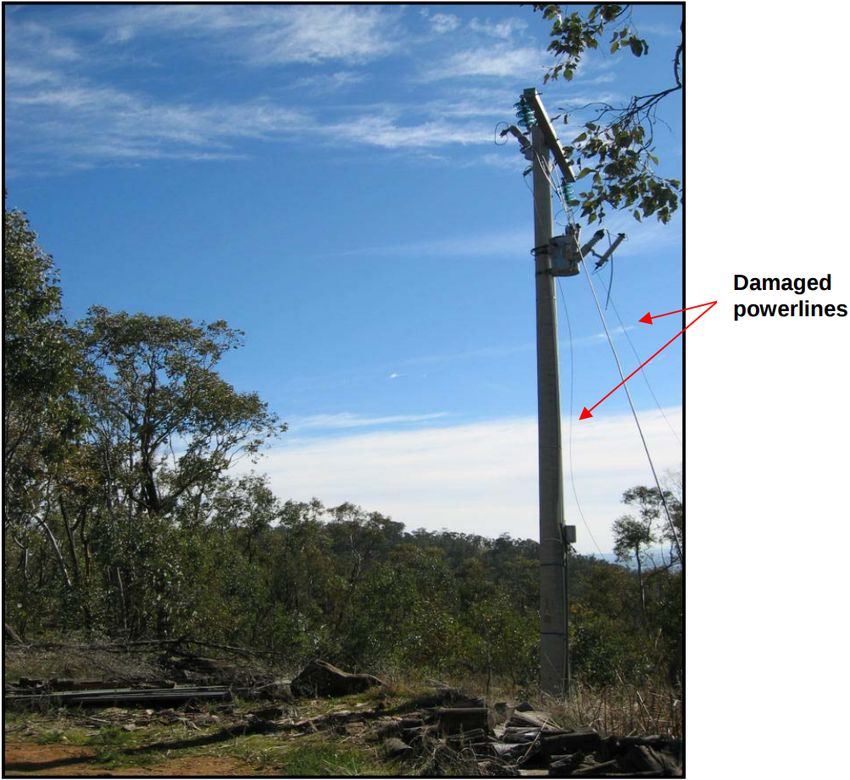
(a) The remains of the helicopter (b) Damaged powerlines
Figure 1.2: Bell 47G-3B-1 Soloy helicopter after striking powerlines near Wodonga on 19 June 2004. Image
from Australian Transport Safety Bureau [2006].
increased to 0.7. There report 169 people involved in the 119 wire-strike accidents,
where the occupant received varying degrees of injury in almost 67 percent of the
cases. There were 45 people fatally injured, 22 seriously injured, and 42 who received
minor injuries.
Aerial agriculture operations accounted for 62 per cent, that is 74 wire-strike acci-
dents. Fixed-wings were involved in 57 per cent of wire-strike accidents and rotary-
wings were involved in the remainer of 43 per cent. Given that fixed-wing aircraft
out number rotary-wing aircraft by seven to one in the Australian aviation industry,
rotary-wing aircraft were over-represented in the data. This data imbalance indicates
that rotary-wing vehicles are involved in higher risk applications.
3Figure 1.3: Thesis outline
1.2 Thesis Overview
Generally, one could use lidar, radar, infrared, electromagnetic sensors or cameras to de-
tect wires and power lines McLaughlin [2006], Sanders-Reed et al. [2009], Luque-Vega et al.
[2014], Matikainen et al. [2016]. While lidar has been shown to work in multiple publica-
tions and products [McLaughlin, 2006, Scherer et al., 2008, Jwa and Sohn, 2012, Cheng
et al., 2014, Ramasamy et al., 2016], for small UAVs it is infeasible due to the high pay-
load and cost of such sensors. To see thin wires which are more than a few meters early
enough so that one has enough time to avoid them, which means that the drone should be
moving slowly enough to obtain a really dense point cloud. Cameras on the other hand
are lightweight, cheap, and can see wires upto long distances.
We propose an approach to detect, reconstruct, and avoid wires using a monocular
camera as our sensor, under the assumption of a known state estimate. Another assumption
is that the RGB image from the camera itself has enough information about the wire that
they can be segmented from the image.
We now delineate our contributions, along with the organization of this thesis
• Wire Segmentation from Monocular Images (Chapter 2)
In this chapter, we present an approach to segment wires from monocular images in a
per-pixel wise fashion. Pixelwise wire detection can be framed as a binary semantic
segmentationtask. Due to the lack of a labeled dataset for this task, we generate
one by rendering photorealistic wires from synthetic models and compositing them
into frames from publicly available flight videos. We show that dilated convolutional
networks trained on this synthetic dataset in conjunction with a few real images
4perform with reasonable accuracy and speed on real-world data on a portable GPU.
This work was published in Madaan et al. [2017].
• Multi-view Reconstruction of Wires using a Catenary Model (Chapter 3)
Given the pixel-wise segmentations, we develop a method for 3D wire reconstruc-
tion. Our method is a model-based multi-view algorithm, which employs a minimal
parameterization of wires as catenary curves. We propose a bundle adjustment-style
framework to recover the model parameters using non-linear least squares optimiza-
tion, while obviating the need to find pixel correspondences by using the distance
transform as our loss function.
• Model-free Mapping and Reactive Avoidance (Chapter 4)
In this section, propose a model-free, implicit voxel-grid mapping method which
uses a pose graphof disparity images to reconstruct both wires from a monocular
segmentations from Chapter 2, and generic obstacles detected from stereo images.
To close the sensing-planning loop for wire avoidance, we demonstrate a reactive,
trajectory library-based planner coupled with the mapping framework in real-world
experiments. This work will be published in [Dubey et al., 2018], and relies heavily
on previous work by Dubey et al. [2017], Dubey [2017].
To get the most out of this thesis, we encourage the reader to visit the corresponding
thesis webpage, which has links to the thesis defence, associated publications and code,
and animation and videos which supplement the figures provided in this document.
56
Chapter 2

Wire Segmentation from Monocular
Images

2.1      Introduction
Thin wires and similar objects like power lines, cables, ropes and fences are one of the
toughest obstacles to detect for autonomous flying vehicles, and are a cause of numerous
accidents each year. They can be especially hard to detect in cases where the background
is cluttered with similar looking edges, when the contrast is low, or when they are of barely
visible thickness. Power line corridor inspection is another area of potentially widespread
application of wire detection capabilities, and leveraging UAVs for this task can save a
lot of money, time, and help avoid dangerous manual labor done by linemen. Apart from
UAVs, there have been recent reports which document fatal injuries and deaths caused by
hitting barbed wire fences while riding ATVs, and dirt and mountain bikes [?]. Generally,
one could use lidar, infrared, electromagnetic sensors or cameras to detect wires and power
lines. Out of these, a monocular camera is the cheapest and most lightweight sensor, and
considering the recent advances in deep learning on images, we use it as our perception
sensor. Apart from a good detection rate, real time performance on a portable GPU like
the NVIDIA Jetson TX2 with a decent resolution like 480x640 is critical to ensure that
wires are still visible in the input image, and that the drone has enough time for potentially
avoiding them.
    Previous work uses strong priors on the nature of power lines - assuming they are
straight lines, have the highest or lowest intensity, appear with a fixed number in an
image, have a gaussian intensity distribution, are the longest line segments, are parallel to
each other, or can be approximated by quadratic polynomials [Kasturi and Camps, 2002,
Candamo et al., 2009, Yan et al., 2007, Li et al., 2010, Sanders-Reed et al., 2009, Song and
Li, 2014]. These works first gather local criteria for potential wire pixels by using an edge
detection algorithm, filter them using the heuristics mentioned above, and then gather
global criteria via variants of the Hough or Radon transform [Kasturi and Camps, 2002,
Candamo et al., 2009, Yan et al., 2007], clustering in space of orientations [Li et al., 2010]
and graph cut models [Song and Li, 2014]. These approaches demand a lot of parameter

                                              7
tuning, work well only in specific scenarios, and are prone to false positives and negatives
since the distinction between wires and other line-like objects in the image does not always
obey the appearance based assumptions and priors.
Another issue with wire detection is the unavailability of a sufficiently large public
dataset with pixel wise annotations. The only existing dataset with a decent number of
labeled images is provided by [Candamo et al., 2009], which we refer to as the USF dataset.
We use it for evaluation of our models, as done by [Song and Li, 2014] as well.
Figure 2.1: A few samples from our synthetically generated dataset along with ground truth labels of
wires. Video examples available at this link and our project page.
We address the former of the aforementioned issues by investigating the effectiveness
of using convolutional neural networks (convnets) for our task. Recent advances in se-
mantic segmentation and edge detection using convnets are an indication of an end to end
wire detection system omitting hand-engineered features and parameter tuning, which can
also potentially generalize to different weather and lighting conditions depending on the
amounts of annotated data available [Long et al., 2015, Bertasius et al., 2015, Xie and
Tu, 2015]. To meet our objectives of real time performance on the TX2 and reasonable
detection accuracy, we perform a grid search over 30 architectures chosen based on our
intuition. We investigate the effect of filter rarefaction [Yu and Koltun, 2015] by system-
atically adding dilated convolutional layers with increasing amounts of sparsity as shown
in Table 2.1 and 2.2. We show that the top 5 models from our grid search outperform
various baselines like E-Net [Paszke et al., 2016], FCN-8 and FCN-16s [Long et al., 2015],
SegNet [Badrinarayanan et al., 2017], and non-deep baseline of [Candamo et al., 2009] as
shown in Fig. 2.4 and Table 2.4 across multiple accuracy metrics and inference speeds on
the Jetson TX2.
To address the latter issue of the unavailability of a large dataset with pixel wise
annotations, we generate synthetic data by rendering wires in 3D as both straight lines
and in their natural catenary curve shape, using the POV-Ray[POV-Ray, 2004] ray-tracing
8engine with varying textures, numbers, orientations, positions, lengths, and light source,
and superimpose them on 67702 frames obtained from 154 flight videos collected from
the internet. A few samples from our dataset can be seen in Figure 2.1 and in the video
here. Although training on synthetic data alone is not enough to match the performance
of models which are finetuned or trained from scratch on the USF dataset, we observe that
synthetic data alone gave pretty accurate qualitative detections on a few unlabeled flight
videos we tested on as shown in Figure 2.5. More results are available at our project page.
Further, for wire detection and avoidance, false negatives (undetected wires) are much
more harmful than false positives. We adapt the line of thought of finding local evidence
and then refining it via heuristics or global criteria used by previous works, to convnets
by explicitly providing local evidence of ‘wiryness’ in the form of extra channels to the
network input. One would expect that doing this would make the network’s task easier as
now it has to filter out the non-wire edges and line segments and return pixels that were
actually wires. However, in the case of training from scratch, or finetuning on the USF
dataset after pretraining on synthetic data, we find that the local primitive information
does not have much effect in the performance of the network. On the other hand, we find
out that adding this information of local criteria does help in the case of models trained
on only synthetic data, as shown in Table 2.2.
In summary, the contributions of this chapter are:
• Systematic investigation of the effectiveness of convnets for wire detection by a grid
search.
• Large scale generation of a synthetic dataset of wires and demonstrating its effective-
ness.
• Investigation of the effect of explicitly providing local evidence of wiryness.
• Demonstrating real time performance on the NVIDIA Jetson TX2 while exceeding
previous approaches both in terms of detection accuracy and inference speed.
Figure 2.2: Close up of synthetic wires rendered using POV-Ray [POV-Ray, 2004].
2.2 Related Work
2.2.1 Wire detection using traditional computer vision
One of the earliest works in wire detection is from [Kasturi and Camps, 2002], who ex-
tract an edgemap using Steger’s algorithm [Steger, 1998], followed by a thresholded Hough
9Table 2.1: The parameter space over which we perform a grid search. Each context module from the 2nd
column was stacked over each front-end module from the first column to get a total of 30 models. All
layers use 3*3 convolutions. Each layer is separted by a ‘-’ sign. ‘k’ refers to the number of channels in
each layer. ‘p’ refers to pooling layers, ‘d’ refers to the dilation factor.
Front-end Modules Context Modules
Key Architecture Key Architecture
f1 k64-k64-p2-k128-k128 c1 k2(none)
f2 k32-k32-k64-k64 c2 d1-d2-d1-k2
f3 k32-k32-k32-k32 c3 d1-d2-d4-d1-k2
f4 k32-k32-k64-k64-k64-k64 c4 d1-d2-d4-d8-d1-k2
f5 k32-k32-k32-k32-k32-k32 c5 d1-d2-d4-d8-d16-d1-k2
f6 k32-k32
transform which rejects lines of short length. However, due to unavailability of ground
truth, they evaluate their approach only on synthetically generated wires superimposed on
real images.
[Candamo et al., 2009] find edges using the Canny detector and then weigh them
proportionally according to their estimated motion found using optical flow, followed by
morphological filtering and the windowed Hough transform. The resulting parameter space
is then tracked using a line motion model. They also introduce the USF dataset and show
that their approach performs better than [Kasturi and Camps, 2002]. We modify their
temporal algorithm to a per-frame algorithm as explained later, and use it as a baseline.
[Song and Li, 2014] proposed a sequential local-to-global power line detection algorithm
which can detect both straight and curved wires. In the local phase, a line segment pool
is detected using Gaussian and first-order derivative of Gaussian filters, following which
the line segments are grouped into whole lines using graph-cut models. They compare
their method explicitly to [Kasturi and Camps, 2002] and their results indicate similar
performance as [Candamo et al., 2009], which is one of our baselines.
2.2.2 Semantic segmentation and edge detection using deep learn-
ing
Fully Convolutional Networks(FCNs) [Long et al., 2015] proposed learned upsampling and
skip layers for the task of semantic segmentation, while SegNet [Badrinarayanan et al.,
2017] proposed an encoder-decoder modeled using pooling indices. For thin wires, FCNs
and SegNet are intuitively suboptimal as crucial information is lost in pooling layers which
becomes difficult to localize in the upsampling layers. E-Net [Paszke et al., 2016] de-
velop a novel architecture by combining tricks from multiple works for real time semantic
segmentation performance, but one of their guiding principles is aggresive downsampling
again.
10Table 2.2: Results of our grid search experiments. The strings in bold, blue text represent the front end
architecture as explained in text. Each front end is appended with five different context modules as shown
in the Col. 1. We conduct six experiments, all of which are evaluated on our test split of the USF dataset.
Each experiment category is grouped with the same hue (Col. 2-3, 4-5, 6-7 respectively). Darker color
implies better performance. Choice of colors is arbitrary. Col. 8-11 list the performance speeds on the
NVIDIA TitanX Pascal and the Jetson TX2, with batch size 1 and input resolution of 480x640.
Average Precision Scores
Performance
(evaluation on USF test split)
Trained On → Synthetic Data Scratch on USF Finetuned on USF TX2 TitanX
Context Module ↓ Time Speed Time Speed
RGB RGBLE RGB RGBLE RGB RGBLE
(ms) (fps) (ms) (fps)
Column 1 2 3 4 5 6 7 8 9 10 11
Front End Module → k32-k32
k2 0.23 0.30 0.45 0.45 0.50 0.47 37.7 26.6 3.2 309.6
d1-d2-d1-k2 0.33 0.35 0.63 0.58 0.61 0.59 115.7 8.7 8.0 124.7
d1-d2-d4-d1-k2 0.28 0.42 0.65 0.61 0.64 0.62 159.3 6.3 10.2 98.0
d1-d2-d4-d8-d1-k2 0.35 0.45 0.65 0.62 0.66 0.65 203.7 4.9 12.4 80.6
d1-d2-d4-d8-d16-d1-k2 0.36 0.49 0.70 0.64 0.70 0.69 249.4 4.0 14.6 68.4
k32-k32-k32-k32
k2 0.24 0.32 0.57 0.50 0.57 0.54 70.7 14.2 5.7 176.1
d1-d2-d1-k2 0.25 0.39 0.62 0.60 0.64 0.59 148.5 6.7 10.1 99.1
d1-d2-d4-d1-k2 0.28 0.40 0.63 0.62 0.66 0.63 192.7 5.2 11.9 83.9
d1-d2-d4-d8-d1-k2 0.33 0.42 0.69 0.62 0.68 0.66 236.6 4.2 13.8 72.6
d1-d2-d4-d8-d16-d1-k2 0.43 0.48 0.70 0.64 0.72 0.64 282.6 3.5 15.7 63.9
k32-k32-k32-k32-k32-k32
k2 0.18 0.35 0.63 0.53 0.61 0.57 104.0 9.6 8.2 121.7
d1-d2-d1-k2 0.30 0.42 0.61 0.58 0.64 0.59 181.5 5.5 13.2 76.1
d1-d2-d4-d1-k2 0.25 0.43 0.62 0.59 0.67 0.62 225.4 4.4 15.3 65.2
d1-d2-d4-d8-d1-k2 0.32 0.47 0.66 0.64 0.70 0.65 270.1 3.7 17.6 57.0
d1-d2-d4-d8-d16-d1-k2 0.03 0.47 0.68 0.66 0.47 0.65 315.0 3.2 19.8 50.6
k32-k32-k64-k64
k2 0.20 0.28 0.59 0.50 0.60 0.55 118.7 8.4 8.3 120.9
d1-d2-d1-k2 0.25 0.45 0.62 0.60 0.62 0.60 350.7 2.9 19.9 50.4
d1-d2-d4-d1-k2 0.29 0.38 0.65 0.62 0.68 0.62 496.2 2.0 26.3 38.1
d1-d2-d4-d8-d1-k2 0.28 0.45 0.66 0.64 0.66 0.64 641.7 1.6 32.8 30.5
d1-d2-d4-d8-d16-d1-k2 0.40 0.48 0.71 0.62 0.71 0.67 787.6 1.3 38.4 26.1
k32-k32-k64-k64-k64-k64
k2 0.27 0.39 0.63 0.57 0.61 0.58 206.6 4.8 13.4 74.8
d1-d2-d1-k2 0.29 0.42 0.62 0.60 0.67 0.59 439.2 2.3 24.7 40.5
d1-d2-d4-d1-k2 0.28 0.38 0.64 0.60 0.65 0.62 582.7 1.7 31.0 32.3
d1-d2-d4-d8-d1-k2 0.37 0.45 0.68 0.62 0.67 0.63 729.8 1.4 37.2 26.9
d1-d2-d4-d8-d16-d1-k2 0.42 0.49 0.68 0.63 0.70 0.63 877.7 1.1 43.9 22.8
k64-k64-p2-k128-k128
k2 0.26 0.35 0.65 0.60 0.66 0.60 136.0 7.4 8.1 124.1
d1-d2-d1-k2 0.30 0.34 0.66 0.63 0.72 0.66 279.8 3.6 17.1 58.5
d1-d2-d4-d1-k2 0.41 0.45 0.70 0.67 0.73 0.67 350.8 2.9 21.8 45.8
d1-d2-d4-d8-d1-k2 0.34 0.49 0.71 0.66 0.73 0.70 421.8 2.4 26.5 37.7
d1-d2-d4-d8-d16-d1-k2 0.36 0.47 0.72 0.64 0.75 0.68 493.2 2.0 31.2 32.0
112.3 Approach
2.3.1 The search for the right architecture
For a wire detection network running on a platform like the NVIDIA TX2 atop a small
UAV, we desire low memory consumption and a fast inference time. Further, as wires
are barely a few pixels wide, we do not want to lose relevant information by the encoder-
decoder approaches [Long et al., 2015, Paszke et al., 2016, Badrinarayanan et al., 2017] in
which one first downsamples to aggregate global evidence and then upsamples back up to
localize the target object.
Dilated convolutional layers [Yu and Koltun, 2015] are a simple and effective way to
gather context without reducing feature map size. Each layer is defined by a dilation factor
of d, which correspond of d − 1 number of alternating zeros between the learnt elements,
as visualized in [Yu and Koltun, 2015, van den Oord et al., 2016]. [Yu and Koltun, 2015]
proposed appending a ‘context module’ comprising of 7 layers with increasing dilation
factors (d for each layer following the series {1,1,2,4,8,16,1}) to existing segmentation
networks (front-end modules), which boosted their performance significantly.
In order to investigate the effect of dilation on our task, we run a grid search over a
finite set of front-end and context modules as summarized in Table 2.1. We now introduce
a simple naming scheme to refer our models with. Each layer is separated by a ‘-’ the
number succeeding ‘k’ is equal to the number of channels, ‘p’ refers to a pooling layer and
‘d’ to a dilation layer. For all layers, we use 3*3 convolutions.
For front-end modules, we begin with trimming down VGG [Simonyan and Zisserman,
2014] to its first two blocks, which is the model f1 in Table 2.1. Next, we halve the number
of channels across f1 and remove the pooling layer to get f2. Then, we halve the number
of channels in the last two layers of f2 of this model to get f3. Further, to investigate the
effect of depth we append 2 layers each to the f2 and f3, while maintaining the number of
channels to get f4 and f5. We stop at 6 layers as previous work [Xie and Tu, 2015] found
it to be enough to detect edges. Finally to check how well a simple two layer front-end
performs, we add f6 to our list. The second column shows the range of the context modules
we evaluated, starting with an empty context module (c1) and building up to c5 as in [Yu
and Koltun, 2015]. Our first model is d1+d2+d1 due to the fact that a dilation factor of
1 is equivalent to standard convolution without holes. Note that there is always a k2 in
the end as in the last layer, we do a softmax operation over two output classes (wire and
not-wire).
By choosing a front-end (f1-f6) and appending it with a context module (c1-c5), we
do a grid search over 30 architectures and do multiple experiments - training each model
on synthetic data, real data, finetuning models trained on synthetic data, and finally
evaluation on real data as shown in Table 2.2. We use a 50-50 train-test split of the USF
dataset for the grid search. We then choose the top 5 models based on the accuracy and
inference speed on the NVIDIA TX2 (bold text in Table 2.3) for comparison with various
baselines.
122.3.2 Generating synthetic data
Due to the unavailaibility of a large dataset with annotations of wires, we render synthetic
wires using the POV-Ray ray tracing engine [POV-Ray, 2004], and superimpose them on
67702 frames sampled from 154 flight videos collected from the internet. Figure 2.1 and
this video shows some examples from our synthetic dataset.
Our dataset consists of wires occuring as both straight lines and catenary curves (the
natural shape of a wire hanged at its ends under uniform gravity). We vary the wire sag,
material properties, light source location, reflection parameters, camera angle, number
of wires and the distance between them across the dataset to obtain a wide variety of
configurations. A close up of the rendered wires can be seen in Figure 2.2.
2.3.3 Class Balancing Loss Function
As wire pixels occupy only a minisicule fraction of the total number of pixels in an image, it
is important to account for class imbalance in the loss function, as well as in the evaluation
metrics used. To that end, we use the image-level, class-balanced cross entropy loss function
defined in [Xie and Tu, 2015]. For the USF dataset, we find that wire pixels account for
only 4.9% of the total number of pixels, and the rest 95.1% are background pixels, and
weigh the loss accordingly.
2.3.4 Explicitly providing local evidence of wires
Previous works extract local evidence of wiryness via edge maps obtained from standard
edge detection algorithms, which is followed by filtering using domain knowledge, and
finally gathering global evidence. We adapt this line of thought to convnets by appending
the results of line segment and edge detection using the recently proposed CannyLines and
CannyPF detectors [Lu et al., 2015] in the form of two additional channels to the network’s
input.
2.4 Experiments and Results
2.4.1 Evaluation Metrics
We first define and justify the metrics used. Average Precision(AP) and Optimal Dataset
Scale(ODS) F1 score are standard metrics used for edge detection tasks Arbelaez et al.
[2011]. AP is defined as the mean precision taken over all recall values, and is equal to the
area under the Precision-Recall(PR) curve. ODS F-score is the optimal F1 score obtained
by choosing the threshold of a probabilistic classifier which gives the best performance
across the training dataset. Previous works on wire detection use the Receiver Operat-
ing Characteristics(ROC) at a per-wire basis. This entails fitting a line or a curve to
thresholded predictions and then counting instances of the same, which leads to ambiguity
due to issues like minimum length to register a detection, choosing polynomials to fit the
thresholded predictions for curved wires, and coming up with tolerances which relax the
13detection criteria. Therefore, we calculate both ROC and PRC on a per-pixel basis and
report Area under the Curve of the ROC diagram(AUC), which like AP, summarizes the
curve with a single number.
It is also worth mentioning that for the case of severely class-imbalanced problems such
as ours, AP is a better performance metric than ROC. In ROC analysis. false detections
are evaluated via False Positive Rate, which compares false positives to true negatives (i.e.
background pixels which account for roughly 95% of the USF dataset). Whereas in PR
curves, the measure of false detections is done by Precision, which compares false positives
to true positives. Therefore, in problems where the negative class outnumbers the positive
class by a huge margin, AP is a better measure for classifier evaluation. We refer the reader
to Davis and Goadrich [2006] for more details.
2.4.2 Grid Search
We do extensive evaluation of the models listed in Table 2.1 on the USF dataset. First,
we randomly select half of the USF videos (21 out of 42 available) for the training set and
kept the rest for testing, leading to 2035 frames for training and 1421 frames for testing.
Meanwhile, we also have a synthetic dataset consisting of 67702 frames from 154 publicly
available flight videos as mentioned before. For all cases, the input resolution used is
480x640. For each model from Table 2.1, we conduct three kind of experiments:
• Synthetic: Train on our synthetic dataset
• Scratch: Train on train split of USF dataset
• Finetune: Finetune on the USF train split after training on synthetic dataset
For each category above, we conduct runs with two different inputs to investigate the
benefits of explicitly providing local evidence:
• RGB: training on monocular images only
• RGBLE: training on monocular images, concatenated with lines(L) and edges(E)
detected by Lu et al. [2015].
Table 2.2 shows the results of all the six experiments on each model, along with the AP
scores and performance on the NVIDIA Titan X Pascal and the TX2. Each experiment
category is assigned an arbitrary hue, and darker color emphasizes better performance.
Same is true for the last 4 columns which depict the inference performance with a batch
size of 1, and input resolution of 480x640. Each class of models with the front-end is
demarked by the bold blue text, while context modules of increasing amount of dilation
are added to them in 5 consecutive rows. From Table 2.2, we can draw the following
conclusions:
• Dilated kernels with increasing sparsity help:
This trend can be seen throughout in Col 2-7 for each front-end. For each column,
for the same frontend module, we can observe increasing AP scores as we add more
dilation in the context modules. As the AP numbers can be close and hard to
judge, we verify the same with Precision Recall curves for each front-end with varying
context modules as shown in Figure 2.3. At the same time, the run-time performance
14of the models decrease as we can keep on adding more layers (Col 8-11).
• Explicitly providing local information only helped in the case of synthetic data:
This can be seen by comparing the RGB and RGBLE columns in Table 2.2 under
each category. In case of training (Col 4-5) or finetuning on real data (Col 6-7), we
actually observe slightly poorer performance by providing results of line and edge
detection. However, for the case of training on synthetic data (Col 2-3), providing
local evidence helps to boost the networks’ performance on real data by fairly big
margins. We believe this is due to the nature of the synthetic dataset which doesn’t
have the same distribution as the USF test split, and hence, giving the networks all
lines and edges explicitly helps to improve their performance. This also suggests that
an RGBLE input might generalize better to a test set having a significantly different
distribution from the training set, but more experimentation is needed to ascertain
that.
• Pretraining on synthetic data helps slightly:
This can be seen by comparing Col 4 with Col 6 (RGB inputs). We believe this is
another artifact of the USF dataset, which is small in size and a lot of images are
relatively simplistic. The previous statement is supported with evidence of results
presented in Fig. 2.5. Here, we train only on synthetic data with 720x1280 resolution,
and tested on a few publicly available videos. In this case, the value of synthetic data
is clearly evident.
For our use case, we desire fast inference speed on the TX2 and decent precision at
high recalls for wires. To pick the best of the lot, the top 15 models from our grid search
experiments on finetuning on the USF dataset with RGB input can be seen in Table 2.3,
along with inference speed with batch size 1 and resolution of 480x640, and number of
parameters (although number of parameters isn’t that much of a burden at inference time
due to enough memory on the TX2). We cherry pick the 5 models in bold text by looking
at these three metrics, the precision recall scores (Fig. 2.4), and qualitative comparisons
(Fig. 2.6). Table 2.4 compares these top-5 models with various baselines.
Implementation details: For training on synthetic data, we use a minibatch size of 4 and
train for 2000 iterations, while for the USF dataset, we train for 1000 iterations. All input
images are of 480x640 resolution. We use AdaDelta Zeiler [2012] we found that stochastic
gradient descent with momentum lead to slower convergence and a few architectures getting
stuck in local minimas. We implement our models in both Lasagne Dieleman et al. [2015]
and Pytorch, as we found that the latter is faster and consumes less memory on the TX2.
2.4.3 Baselines
We consider four baselines to compare our approach with - Candamo et al.Candamo et al.
[2009], FCNsLong et al. [2015], SegNetBadrinarayanan et al. [2017] and E-NetPaszke et al.
[2016]. We adapt the temporal approach of Candamo et al. [2009] described in the related
work section to a per-frame method: first we perform edge detection using Lu et al. [2015],
followed by morphological filtering of 8-connected components with connectivity of less
15Table 2.3: Top models from our grid search. All models were trained on synthetic data first, then finetuned
on our USF dataset test split using RGB input. Darker color in each colum implies higher accuracy, higher
speed (frames per second) on the TX2, and smaller number of model parameters. Hues for each column
are chosen arbitrarily.
Model AP Score TX2 Number
(Finetune RGB) (fps) of params
k64-k64-p2-k128-k128-d1-d2-d4-d8-d16-d1-k2 0.75 2.03 1,147,970
k64-k64-p2-k128-k128-d1-d2-d4-d1-k2 0.73 2.85 852,802
k64-k64-p2-k128-k128-d1-d2-d4-d8-d1-k2 0.73 2.37 1,000,386
k32-k32-k32-k32-d1-d2-d4-d8-d16-d1-k2 0.72 3.54 84,706
k64-k64-p2-k128-k128-d1-d2-d1-k2 0.72 3.57 705,218
k32-k32-k64-k64-d1-d2-d4-d8-d16-d1-k2 0.71 1.27 288,290
k32-k32-d1-d2-d4-d8-d16-d1-k2 0.70 4.01 66,210
k32-k32-k32-k32-k32-k32-d1-d2-d4-d8-d1-k2 0.70 3.7 93,954
k32-k32-k64-k64-k64-k64-d1-d2-d4-d8-d16-d1-k2 0.70 1.14 362,146
k32-k32-k32-k32-d1-d2-d4-d8-d1-k2 0.68 4.23 75,458
k32-k32-k64-k64-d1-d2-d4-d1-k2 0.68 2.02 214,434
k32-k32-k32-k32-k32-k32-d1-d2-d4-d1-k2 0.67 4.44 84,706
k32-k32-k64-k64-k64-k64-d1-d2-d1-k2 0.67 2.28 251,362
k32-k32-k64-k64-k64-k64-d1-d2-d4-d8-d1-k2 0.67 1.37 325,218
16Table 2.4: Our top models compared with various baselines. The metrics used are Average Precision(AP),
Area under the Curve of ROC diagram(AUC), Optimal Dataset Scale F1-Score(ODS F-Score)
ODS TX2
Model AP AUC
F-Score (fps)
FCN-8 Long et al. [2015] 0.581 0.960 0.598 1.37
FCN-16 Long et al. [2015] 0.639 0.972 0.663 1.39
Segnet Badrinarayanan et al. [2017] 0.571 0.939 0.567 2.19
Candamo Candamo et al. [2009] 0.408 - 0.382 -
E-Net Paszke et al. [2016] 0.580 0.945 0.595 -
k64-k64-p2-k128-k128-
0.729 0.972 0.688 2.85
d1-d2-d4-d1-k2
k32-k32-k32-k32-
0.717 0.976 0.678 3.54
d1-d2-d4-d8-d16-d1-k2
k32-k32-
0.703 0.969 0.673 4.01
d1-d2-d4-d8-d16-d1-k2
k32-k32-k32-k32-k32-k32-
0.696 0.973 0.656 3.70
d1-d2-d4-d8-d1-k2
k32-k32-k32-k32-k32-k32-
0.667 0.970 0.647 4.44
d1-d2-d4-d1-k2
than 30 pixels, followed by a windowed Hough transform by breaking up the edgemap
image into 16 (4*4) subwindows.
Table 2.4 and Figure 2.4 shows the performance of our top 5 models along with the
baselines. We report AP, AUC, ODS-F1 scores, inference speed for a 480x640 image with
batch size 1 on the NVIDIA TX2, and the PR curves. For Candamo et al. [2009], as the
output is a binary prediction (detected lines via windowed Hough transform) and not a
confidence value as in the case of CNNs, we report the F1 score and the Precision value in
the ODS F-score and the AP fields respectively. We don’t report AUC as that is applicable
to probabilistic classifiers only. To calculate the metrics in this case, we rasterize the results
of the Hough transform with varying thickness of the plotted lines from 1 to 5 pixels and
report the best F1 and Precision scores obtained for a fair comparison.
2.5 Conclusion and Future Work
In this paper, we presented a method to detect wires using dilated convnets to facilitate
autonomous UAVs. We generate a large synthetic dataset by rendering wires and superim-
posing them on frames of publicly available flight videos, and demonstrate its effectiveness
by showing qualitative and quantitative results. Our experiments systematically find the
best architectures over a finite space of model parameters and outperform various baselines
across multiple detection metrics and inference speeds on the NVIDIA TX2.
We are currently working on multi-view stereo methods to find distance of the wires
and coming up with methods to avoid them robustly at high speeds. For improving the
perception pipeline, we are looking into eliminating false positives and considering temporal
17You can also read