A climatological benchmark for operational radar rainfall bias reduction
←
→
Page content transcription
If your browser does not render page correctly, please read the page content below
Hydrol. Earth Syst. Sci., 25, 4061–4080, 2021
https://doi.org/10.5194/hess-25-4061-2021
© Author(s) 2021. This work is distributed under
the Creative Commons Attribution 4.0 License.

A climatological benchmark for operational radar
rainfall bias reduction
Ruben Imhoff1,2 , Claudia Brauer1 , Klaas-Jan van Heeringen2 , Hidde Leijnse1,3 , Aart Overeem1,3 , Albrecht Weerts1,2 ,
and Remko Uijlenhoet1,4
1 Hydrology and Quantitative Water Management Group, Wageningen University & Research, Wageningen, the Netherlands
2 OperationalWater Management & Early Warning, Department of Inland Water Systems, Deltares, Delft, the Netherlands
3 R&D Observations and Data Technology, Royal Netherlands Meteorological Institute, De Bilt, the Netherlands
4 Department of Water Management, Delft University of Technology, Delft, the Netherlands

Correspondence: Ruben Imhoff (ruben.imhoff@deltares.nl)

Received: 19 February 2021 – Discussion started: 25 February 2021
Revised: 11 June 2021 – Accepted: 15 June 2021 – Published: 13 July 2021

Abstract. The presence of significant biases in real-time        rable to the reference and outperform the MFB-adjusted rain-
radar quantitative precipitation estimations (QPEs) limits its   fall estimates for catchments away from the radars, where
use in hydrometeorological forecasting systems. Here, we         the MFB-adjusted QPE generally underestimates the rainfall
introduce CARROTS (Climatology-based Adjustments for             amounts. This difference is absent for catchments closer to
Radar Rainfall in an OperaTional Setting), a set of fixed bias   the radars. QPE underestimations are amplified when used in
reduction factors, which vary per grid cell and day of the       the hydrological model simulations. Discharge simulations
year. The factors are based on a historical set of 10 years of   using the QPE from CARROTS outperform those with the
5 min radar and reference rainfall data for the Netherlands.     MFB-adjusted product for all but one basin. Moreover, the
CARROTS is both operationally available and independent          proposed factor derivation method is robust. It is hardly sen-
of real-time rain gauge availability and can thereby provide     sitive to leaving individual years out of the historical set and
an alternative to current QPE adjustment practice. In addi-      to the moving window length, given window sizes of more
tion, it can be used as benchmark for QPE algorithm devel-       than a week.
opment. We tested this method on the resulting rainfall es-
timates and discharge simulations for 12 Dutch catchments
and polders. We validated the results against the operational
mean field bias (MFB)-adjusted rainfall estimates and a ref-     1   Introduction
erence dataset. This reference consists of the radar QPE, that
combines an hourly MFB adjustment and a daily spatial ad-        Radar rainfall estimates are essential for hydrometeorologi-
justment using observations from 32 automatic and 319 man-       cal forecasting systems. In these systems, the data are used
ual rain gauges. Only the automatic gauges of this network       to force hydrological models (e.g., Borga, 2002; Thorndahl
are available in real time for the MFB adjustment. The result-   et al., 2017), to initialize numerical weather prediction mod-
ing climatological correction factors show clear spatial and     els (e.g., Haase et al., 2000; Rogers et al., 2000) or as in-
temporal patterns. Factors are higher away from the radars       put data for rainfall nowcasting techniques (e.g., Ebert et al.,
and higher from December through March than in other sea-        2004; Wilson et al., 2010; Foresti et al., 2016; Heuvelink
sons, which is likely a result of sampling above the melting     et al., 2020; Imhoff et al., 2020a). A major disadvantage of
layer during the winter months. The MFB-adjusted QPE out-        radar quantitative precipitation estimations (QPEs) are the
performs the CARROTS-corrected QPE when the country-             considerable biases with respect to the true rainfall, caused
average rainfall estimates are compared to the reference.        by three main groups of errors: (1) sources of errors re-
However, annual rainfall sums from CARROTS are compa-            lated to the reflectivity measurements, (2) sources of errors
                                                                 in the conversion from reflectivity to rainfall rate and (3)

Published by Copernicus Publications on behalf of the European Geosciences Union.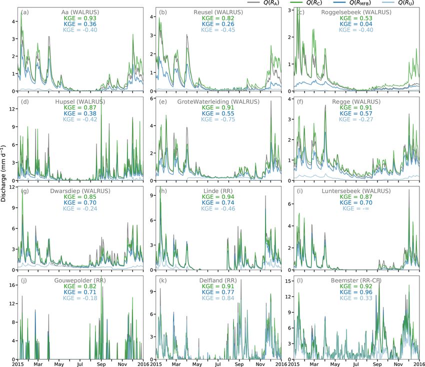
4062                            R. Imhoff et al.: A climatological benchmark for operational radar rainfall bias reduction

spatiotemporal sampling errors (Austin, 1987; Joss and Lee,           In addition, two potential operational (forecasting) issues
1995; Creutin et al., 1997; Gabella et al., 2000; Sharif et al.,   need to be considered when using these more advanced geo-
2002; Uijlenhoet and Berne, 2008; Ochoa-Rodriguez et al.,          statistical and Bayesian merging methods: (1) the methods
2019; Imhoff et al., 2020b). These biases can be amplified         are computationally expensive, especially methods such as
when used in hydrological models (Borga, 2002; Borga et al.,       co-kriging and Bayesian merging that integrate radar and rain
2006; Brauer et al., 2016). Hence, radar QPE requires cor-         gauges (Ochoa-Rodriguez et al., 2019), and (2) when the ad-
rections before operational use in hydrometeorological (fore-      justment method changes the spatial structure of the origi-
casting) models.                                                   nal radar rainfall fields (kriging and Bayesian methods), this
   A large number of correction methods are already avail-         may impact the continuity of the rainfall fields over time and
able. These methods range from corrections prior to the rain-      thereby also the radar rainfall nowcasts (Ochoa-Rodriguez
fall estimations, e.g., corrections for physical phenomena         et al., 2013; Na and Yoo, 2018). In the case that the nowcasts
such as ground clutter, attenuation, the vertical profile of       suffer from errors due to these adjustments, adjustment meth-
reflectivity (VPR) and variations in raindrop size distribu-       ods should be applied to the nowcasts as a post-processing
tion (e.g., Joss and Pittini, 1991; Germann and Joss, 2002;        step. To do this, the forecaster would need to estimate the fu-
Berenguer et al., 2006; Cho et al., 2006; Uijlenhoet and           ture (bias) correction factors (a method for this using MFB
Berne, 2008; Kirstetter et al., 2010; Qi et al., 2013; Hazen-      adjustment is described in Seo et al., 1999) or simply assume
berg et al., 2013, 2014), to statistical post-processing steps     that the latest correction factors are exemplary for the coming
for bias removal in the radar QPE using rain gauge data.           hours.
These post-processing methods either merge rain gauge and             Hence, operational hydrometeorological forecasting calls
radar QPE from the same interval or base correction factors        for a radar rainfall adjustment approach that (1) takes the
on the total precipitation in both products over a past period,    spatial variability in radar QPE errors into account and (2)
such as a number of rainy days (e.g., 7 d in Park et al., 2019).   is available in real time so that it can be used operationally
An often used method is the mean field bias (MFB) correc-          for radar-based rainfall forecasts, such as nowcasting. Here,
tion method, which determines a spatially averaged correc-         we present CARROTS (Climatology-based Adjustments for
tion factor from the ratio between rain gauge observations         Radar Rainfall in an OperaTional Setting), a set of grid-
and the radar QPE of the superimposed grid cells at the lo-        ded climatological adjustment factors for every day of the
cations of these gauges (Smith and Krajewski, 1991; Seo            year, based on a historical set of 10 years of 5 min radar
et al., 1999). This method, which is used operationally in         and reference rainfall data for the Netherlands. When suf-
the Netherlands and many other countries (Holleman, 2007;          ficient rain gauges are operationally available, which would
Harrison et al., 2009; Thorndahl et al., 2014; Goudenhoofdt        allow for a robust application of more advanced geostatisti-
and Delobbe, 2016), does not account for any spatial vari-         cal and Bayesian merging methods, CARROTS can serve as
ability in the radar QPE bias, even though the bias is known       a benchmark for testing these and other more sophisticated
to increase with increasing distance from the radar (Koisti-       adjustment techniques.
nen and Puhakka, 1981; Joss and Lee, 1995; Koistinen et al.,
1999; Gabella et al., 2000; Michelson and Koistinen, 2000;
Seo et al., 2000).                                                 2     Data and methods
   It is possible to account for this spatial variability with
geostatistical techniques (e.g., ordinary kriging, kriging with    2.1    Radar rainfall estimates
external drift or co-kriging; Krajewski, 1987; Creutin et al.,
1988; Wackernagel, 2003; Schuurmans et al., 2007; Gouden-          The archive (2009–2018) of radar rainfall composites in this
hoofdt and Delobbe, 2009; Sideris et al., 2014) or Bayesian        study originates from two C-band weather radars operated by
merging methods (Todini, 2001). Although these methods             KNMI (Fig. 1). Between September 2016 and January 2017,
substantially improve the QPE in the spatial domain, all           both radars were replaced by dual-polarization radars, and
gauge-based radar QPE adjustment methods are limited by            the radar in De Bilt (“DB” in Fig. 1) was replaced by a new
the timely availability of sufficient, and ideally quality-        one in Herwijnen (“H” in Fig. 1). The radar renewals and
controlled, rain gauge observations (for an overview of meth-      relocation have had a limited impact on the QPE product,
ods and their limitations, see Ochoa-Rodriguez et al., 2019).      mainly because the operational products are not yet (fully)
The gauge networks operated by the Royal Netherlands Me-           using the additional information from the dual-polarization
teorological Institute (KNMI) are an example of this issue.        (Beekhuis and Holleman, 2008; Beekhuis and Mathijssen,
Although there is approximately one station per 100 km2 ,          2018).
only 32 out of 351 rain gauges operate automatically. The             The radar product is Doppler-filtered for ground clut-
remaining 319 manual rain gauges report just once a day.           ter. This product is then used to construct horizontal cross-
Thus, only the automatic rain gauges are used for the MFB          sections at a nearly constant altitude of 1500 m, called
adjustment that takes place every hour in real time (Holle-        pseudo-constant plan position indicators (pseudo-CAPPIs).
man, 2007) and recently even every 5 min.                          Subsequently, range-weighted compositing is used to com-

Hydrol. Earth Syst. Sci., 25, 4061–4080, 2021                                       https://doi.org/10.5194/hess-25-4061-2021
R. Imhoff et al.: A climatological benchmark for operational radar rainfall bias reduction                                               4063

Figure 1. Overview of the basins in this study: (a) study area with the location of the three radars (green triangles) operated by KNMI and the
12 basins (orange polygons). The two grey circles indicate a range of 100 km around the radars in Den Helder (DH) and Herwijnen (H). The
other radar (DB) is the radar in De Bilt, which was used until January 2017 and replaced by the radar in Herwijnen. Note that the range used
in the composite was more than 100 km, but 100 km is often regarded as the distance up to which the radar QPE is expected to be reliable.
(b) Locations of the 32 automatic and 319 manual rain gauges currently operated by KNMI. Note that the number of rain gauges has slightly
changed from 2009 until present. (c) List of the basin names, sizes, number of gauges in the basin and hydrological models employed. The
numbers in the left column refer to the numbers in (a). The right column states the used model for these areas.

bine the reflectivities from both radars (Overeem et al.,                    In this equation, Zh is the reflectivity at horizontal polar-
2009b). Since 2013, non-meteorological echoes have been                   ization (mm6 m−3 but generally given in dBZ, according to
removed as an additional step with a cloud mask obtained                  10 × log10 [Zh ]), and R is the rainfall rate (mm h−1 ). The fi-
from satellite imagery. As a final step, rainfall rates are esti-         nal product is called the unadjusted radar QPE (RU ) in this
mated with a fixed Z–R relationship (Marshall et al., 1955):              study.
                                                                             KNMI also provides adjusted radar rainfall products,
Zh = 200R 1.6 .                                                  (1)      based on the aforementioned product, but adjusted with
                                                                          quality-controlled observations from both 32 automatic

https://doi.org/10.5194/hess-25-4061-2021                                               Hydrol. Earth Syst. Sci., 25, 4061–4080, 2021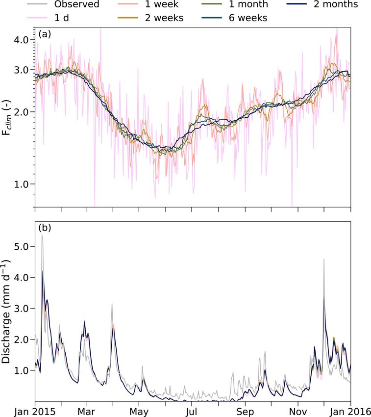
4064                               R. Imhoff et al.: A climatological benchmark for operational radar rainfall bias reduction

Table 1. Statistics of Fig. 2. Indicated are the sample size, the slope
of a linear fit between the two rainfall products (RA and RU ; the
dashed colored lines in Fig. 2) for all observations and the Pearson
correlation coefficient. This is indicated per season (DJF is winter,
MAM is spring, JJA is summer and SON is autumn) and for all
seasons together (Total).

       Season     Sample size     Slope        Pearson      R2
                                            correlation
       DJF                902      0.35           0.90     0.81
       MAM                920      0.48           0.89     0.79
       JJA                920      0.50           0.89     0.79
       SON                910      0.45           0.92     0.85
       Total             3652      0.45           0.89     0.79

hourly and 319 manual daily rain gauges (Overeem et al.,
2009a, b, 2011; note that the number of rain gauges has
slightly changed from 2009 until present). The same 32 auto-
matic rain gauges are used for the MFB-adjustment method,
which will be introduced in Sect. 2.2.1. In contrast to the spa-          Figure 2. The systematic discrepancy between the reference rain-
tially uniform hourly MFB adjustment, the observations from               fall (RA ) and the unadjusted radar QPE (RU ). Shown are the daily
the manual rain gauges are used for daily spatial adjustments,            country-average rainfall sums based on 10 years (2009–2018), clas-
based on distance-weighted interpolation of these observa-                sified per season. The slope, Pearson correlation and sample size
tions (Barnes, 1964; Overeem et al., 2009b). See Sect. 2.2.3              per season are indicated in Table 1. The dashed colored lines are
for a more detailed description of this method.                           a linear fit, forced through the origin, per season between RA and
                                                                          RU .
   This product is considered as a reference rainfall product
in the Netherlands, and it is therefore also regarded as the
reference here (referred to as RA in this study). The RA data
                                                                          than during the other seasons (50 %–55 %). In the follow-
are not available in real time (available with a delay of 1 to
                                                                          ing two subsections, the operationally used MFB-adjustment
2 months because they only use quality-controlled and vali-
                                                                          method and the CARROTS method proposed in this study
dated rain gauge observations), but they are archived and can
                                                                          will be introduced.
therefore be used for “offline” methods. Both RA and RU
have a 1 km2 spatial and 5 min temporal resolution.                       2.2.1   Mean field bias adjustment
   The year 2008 is actually the first year in the KNMI
archive of both datasets, but it was left out of the analysis             The mean field bias (MFB) adjustment method is the oper-
here. RU for this year showed a significantly different behav-            ational adjustment technique in the Netherlands, and it was
ior than the other years, especially during the first half year in        used in this study for comparison with the proposed clima-
which the product rarely underestimated and frequently even               tological bias reduction method (Sect. 2.2.2). This method
overestimated the rainfall sums. The reason for this behavior             provides a spatially uniform multiplicative adjustment fac-
is not yet fully understood. KNMI (2009) reported that spring             tor that is applied to RU . The adjustment factor (FMFB ) was
was exceptionally dry in the north of the country and that the            calculated as (Holleman, 2007; Overeem et al., 2009b)
months January and May were among the warmest on record.
                                                                                     N
On some days with overestimations, clear bright band effects                         P
                                                                                          G(in , jn )
were visible in the radar mosaic, which may have contributed                        n=1
to the systematic differences.                                            FMFB =                          ,                              (2)
                                                                                    N
                                                                                    P
                                                                                          RU (in , jn )
2.2    Bias correction factors                                                      n=1

                                                                          with G(in , jn ) the hourly rainfall sum for gauge n at location
Figure 2 indicates the need for correction of the real-time
                                                                          (in , jn ) and RU (in , jn ) the unadjusted hourly rainfall sum for
available radar rainfall product. RU systematically underesti-
                                                                          the corresponding radar grid cell. The calculation of FMFB
mates the true rainfall amounts, averaged for the land surface
                                                                          was only performed when both the rainfall sum of all rain
area of the Netherlands, by 55 %. This bias is not uniform
                                                                          gauges together and the sum of all corresponding radar grid
in space, as will be highlighted in Sect. 3, and in time with
                                                                          cells were at least 1.0 mm. In all other cases, FMFB = 1.0.
higher underestimations during winter (on average 65 %)

Hydrol. Earth Syst. Sci., 25, 4061–4080, 2021                                                 https://doi.org/10.5194/hess-25-4061-2021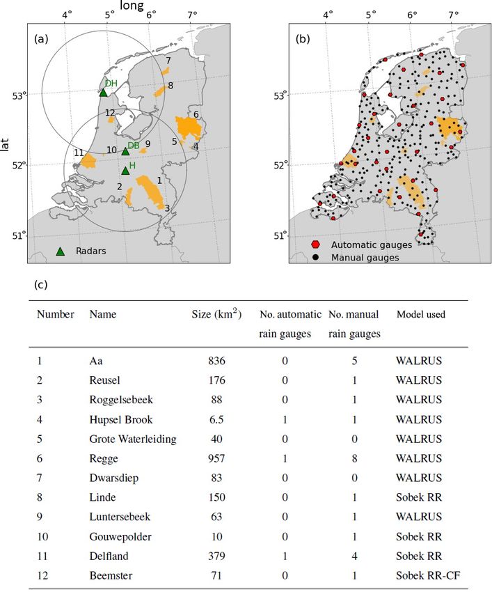
R. Imhoff et al.: A climatological benchmark for operational radar rainfall bias reduction                                      4065

   The MFB-adjustment factors were determined from the              and (3) spatial adjustment of the hourly or higher frequency
1 h accumulations of both RU and the 32 automatic rain              MFB-adjusted rainfall fields (step 1) using the spatial adjust-
gauges, as only the automatic gauges were operationally             ment from step 2.
available every hour (Holleman, 2007; Overeem et al.,                 A spatial adjustment factor (step 2) is derived per grid cell
2009b). The adjustment factors at the temporal resolution of        as follows (for a more elaborate description, see Sect. 3 in
the radar QPE (5 min) were assumed to equal the 1 h adjust-         Overeem et al., 2009a, b):
ment factors for a given hour.                                                   PN
   Moreover, this analysis took place with archived datasets,                          wn (i, j ) · G(in , jn )
                                                                    FS (i, j ) = PNn=1                           ,              (4)
which were validated and consisted of quality-controlled rain                     n=1 wn (i, j ) · RU (in , jn )
gauge observations. It is noteworthy that the same quality
                                                                    with N the number of radar–gauge pairs, G(in , jn ) the daily
control is absent and that missing data occur in real time,
                                                                    rainfall sum for manual rain gauge n at location (in , jn ) and
which can lead to deteriorating results when the MFB ad-
                                                                    RU (in , jn ) the unadjusted daily rainfall sum for the corre-
justment is applied in an operational test case.
                                                                    sponding radar grid cell. wn (i, j ) is a weight for gauge n,
2.2.2   CARROTS method                                              based on the following function:
                                                                                         dn2 (i,j )
                                                                                     −
To derive the climatological bias correction factors for the        wn (i, j ) = e          σ2        .                           (5)
CARROTS method, both RU and RA were used for the years
2009–2018. The use of the reference data for this method               Here, dn2 (i, j ) is the squared distance between gauge n and
was possible because the CARROTS method did not require             the grid cell for which the factor is derived. σ determines the
a real-time availability of the data. The bias correction factors   smoothness of the adjustment factor field. It was set to 12 km
were determined per grid cell in the radar domain according         by Overeem et al. (2009a, b), based on the average gauge
to the following three steps:                                       spacing in the Netherlands.
                                                                       Finally, to spatially adjust the hourly MFB-adjusted rain-
  1. For every day in the period 2009–2018, all 5 min rainfall      fall fields (step 3), two more steps are followed. First, the
     sums (both RU and RA ) within a moving window of               hourly MFB-adjusted rainfall fields (see Sect. 2.2.1 for the
     31 d (the day of interest plus the 15 d before and after       MFB-adjustment method) are accumulated to daily sums.
     it) were summed. The purpose of the moving window              For each grid cell, a new adjustment field is then determined:
     was to smooth the systematic day-to-day variability of                                 RS (i, j )
     the estimated rainfall in the 10-year data. Sections 2.4       FMFBS (i, j ) =                     ,                         (6)
                                                                                           RMFB (i, j )
     and 3.4 describe a leave-one-year-out validation of the
     method, and they describe the sensitivity of the method        with RS (i, j ) the spatially adjusted daily sum for grid cell
     to the moving window size.                                     (i, j ) obtained using Eq. (4) and RMFB (i, j ) the MFB-
                                                                    adjusted daily sum for grid cell (i, j ). Second, the 1 h or
  2. For every day of the year, the 31 d sums around that day       higher frequency (5 min in this study) MFB-adjusted rainfall
     were averaged over the 10 years. Thus, the value for,          fields are multiplied by the adjustment factor FMFBS (i, j ).
     e.g., 16 January consisted of the average 31 d sum for
     the period 1 to 31 January over the 10 years. Leap years       2.3   Hydrometeorological application
     are left out of this analysis due to the low number of
     leap years in the studied period.                              Both bias adjustment methods were applied to the 10 years
                                                                    (2009–2018) of RU . In order to provide a hydrometeorolog-
  3. Finally, gridded climatological adjustment factors             ical testbed, both the CARROTS and MFB-adjusted QPE
     (Fclim ) were calculated per day of the year as                products (from here on referred to as RC and RMFB , respec-
                                                                    tively) were validated against the reference rainfall. First, this
                       RA (i, j )
     Fclim (i, j ) =              ,                          (3)    was done at country level. The estimated daily rainfall sums
                       RU (i, j )                                   for all grid cells within the land surface area of the Nether-
     with RA (i, j ) the reference rainfall sum and RU (i, j )      lands were compared to the reference in a similar way as
     the unadjusted (operational) radar rainfall sum at grid        the comparison in Fig. 2. To subdivide these results per year
     cell (i, j ) for the 10 years.                                 and season, an additional hourly rainfall sum validation was
                                                                    performed as well. The results of this analysis can be found
2.2.3   Spatial adjustments for the reference product               in the Appendix, and the analysis was done as follows: for
                                                                    every rainy hour (when the sum of at least one grid cell was
The adjustment procedure to derive RA consists of three             larger than 0.0 mm), we computed the root mean square error
steps: (1) mean field bias correction (one adjustment factor        (RMSE) by squaring the differences between the three QPE
for the whole country which varies per hour; see Sect. 2.2.1),      products (RU , RC and RMFB ) on the one hand and the ref-
(2) derivation of a daily spatial adjustment factor per grid cell   erence on the other and taking the average of these squared

https://doi.org/10.5194/hess-25-4061-2021                                            Hydrol. Earth Syst. Sci., 25, 4061–4080, 2021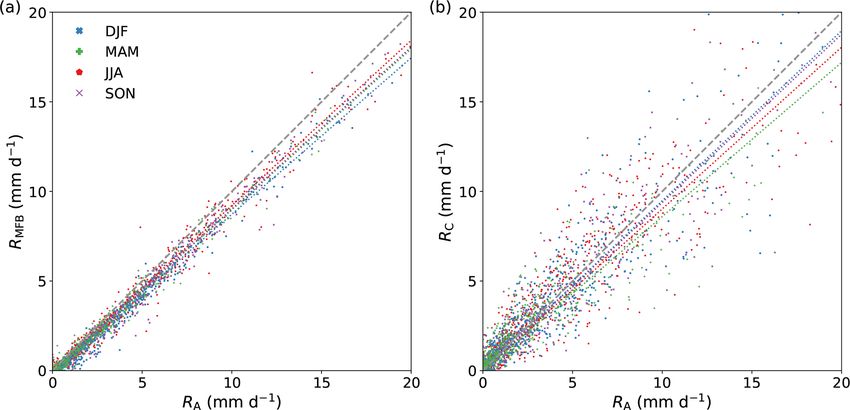
4066                           R. Imhoff et al.: A climatological benchmark for operational radar rainfall bias reduction

differences over all grid cells within the land surface area of      Here, ρ is the Pearson correlation between observed and
the Netherlands. Subsequently, the RMSE was averaged over         simulated discharge, α the flow variability error between ob-
all rainy hours in that season and year. Finally, the seasonal    served and simulated discharge and β the bias between mean
mean RMSE was divided by the average hourly rainfall rate         simulated (µs ) and mean observed (µo ) discharge. σs and σo
for that season and year, resulting in the fractional standard    are the standard deviations of the simulated and observed dis-
error (FSE) score. The FSE score was calculated for every         charge. The KGE metric ranges from −∞ to 1.0, with 1.0
season in the 10 years to be able to compare the seasonal         representing a perfect agreement between observations and
performance of the hourly rainfall estimates of RU , RC and       simulations. In this study, the discharge simulated with RA
RMFB .                                                            as input was regarded as the observation.
   Second, the annual rainfall sums for 12 basins (a combi-          Note that this validation method was not a leave-one-out or
nation of catchments and polders) in the Netherlands (Fig. 1)     split-sample validation, as the full 10-year dataset was used
were compared with the reference. In addition, RC and RMFB        for RA and the CARROTS- and MFB-adjustment derivation,
were used as input for the rainfall-runoff models of the 12       and shorter periods in those 10 years were used for hydrolog-
basins. Most of the involved water authorities use these (low-    ical model calibration. However, the sensitivity of the CAR-
land) rainfall-runoff models either operationally or for re-      ROTS factor was tested by leaving individual years out of the
search purposes, often embedded in a Delft-FEWS system,           derivation period (Sect. 2.4).
which is a data-integration platform used worldwide by many
hydrological forecasting agencies and water management or-        2.4    Sensitivity analysis
ganizations that brings data handling and model integration
together for operational forecasting (Werner et al., 2013). For   As mentioned in Sect. 2.2.2, the purpose of the 31 d moving
this reason, most models were already calibrated using inter-     window in the factor derivation of CARROTS was to smooth
polated rain gauge data or the RA product (e.g. Brauer et al.,    the day-to-day variability of rainfall. To test the sensitivity
2014b; Sun et al., 2020). The calibration period was based        of the method to the employed moving window size, the ad-
on the availability and quality of discharge observations for     justment factors were re-derived for a range of moving win-
that basin, but it was generally 1 to 2 years within the period   dow sizes (1 d, 1 week, 2 weeks, 6 weeks and 2 months).
considered in this study (2009–2018). The WALRUS mod-             The derived factors were then compared to the original fac-
els for catchments Roggelsebeek and Dwarsdiep were not            tor in this study, which was based on a moving window size
calibrated prior to this study and were therefore calibrated      of 31 d, and used to derive adjusted QPE products. Subse-
with the reference data (RA ) for the periods 2013–2014           quently, these QPE products served as input for 1 of the 12
(Roggelsebeek) and 2016–2017 (Dwarsdiep). The choice for          catchments, namely the WALRUS model for the Aa catch-
these periods was based on discharge observation availability     ment (Fig. 1), to test the effect on the simulated discharges
and quality. The employed SOBEK RR(-CF) model (Stelling           (see Sect. 3.4 and Fig. 8 for the results). The Aa catchment
and Duinmeijer, 2003; Stelling and Verwey, 2006; Prinsen          was chosen because the unadjusted QPE product (RU ) for
et al., 2010) is semi-distributed, and therefore we used sub-     this catchment has one of the highest biases of the 12 studied
catchment-averaged rainfall sums from the gridded radar           catchments (see Sect. 3 and Fig. 4).
QPE. The four basins with a SOBEK model have the fol-                Besides the moving window choice, the length of the radar
lowing number of sub-catchments: 7 for Gouwepolder, 1             rainfall archive (10 years) was finite. To test whether or not
for Beemster, 25 for Delfland and 23 for Linde. WALRUS            this archive length was sufficient for reaching a stable factor
(Brauer et al., 2014a) is lumped, so the catchment-averaged       derivation, individual years in the 10-year archive were left
radar QPE was used as input. A more detailed description of       out of the CARROTS method. Hence, the adjustment factors
both rainfall-runoff models is outside the scope of this paper.   were recalculated 10 times in a leave-one-year-out method,
All 12 model setups were run with a 5 min time step for the       applied to RU and used as input for the WALRUS simulations
period 2009–2018.                                                 for the Aa catchment. See Sect. 3.4 and Fig. 4 for the results.
   The resulting discharge simulations were validated for the
same period and 5 min time step using the Kling–Gupta effi-       3     Results
ciency (KGE) metric (Gupta et al., 2009):
            q                                                     3.1    Seasonal and spatial variability
KGE = 1 −       (ρ − 1)2 + (α − 1)2 + (β   − 1)2 ,         (7)
                                                                  The adjustment factors from CARROTS present the spatial
                                                                  variability in the radar QPE errors, with generally higher
with
                                                                  adjustment factors towards the edges of the radar domain
   σs                                                             (Fig. 3). This difference is most pronounced from December
α=    ,                                                    (8)    through March, with factors in the south and east of the coun-
   σo
   µs                                                             try more than 2 times higher than in the central and north-
β=     .                                                   (9)    western parts (Fig. 3a, b and l). Figure 3 demonstrates a clear
   µo

Hydrol. Earth Syst. Sci., 25, 4061–4080, 2021                                      https://doi.org/10.5194/hess-25-4061-2021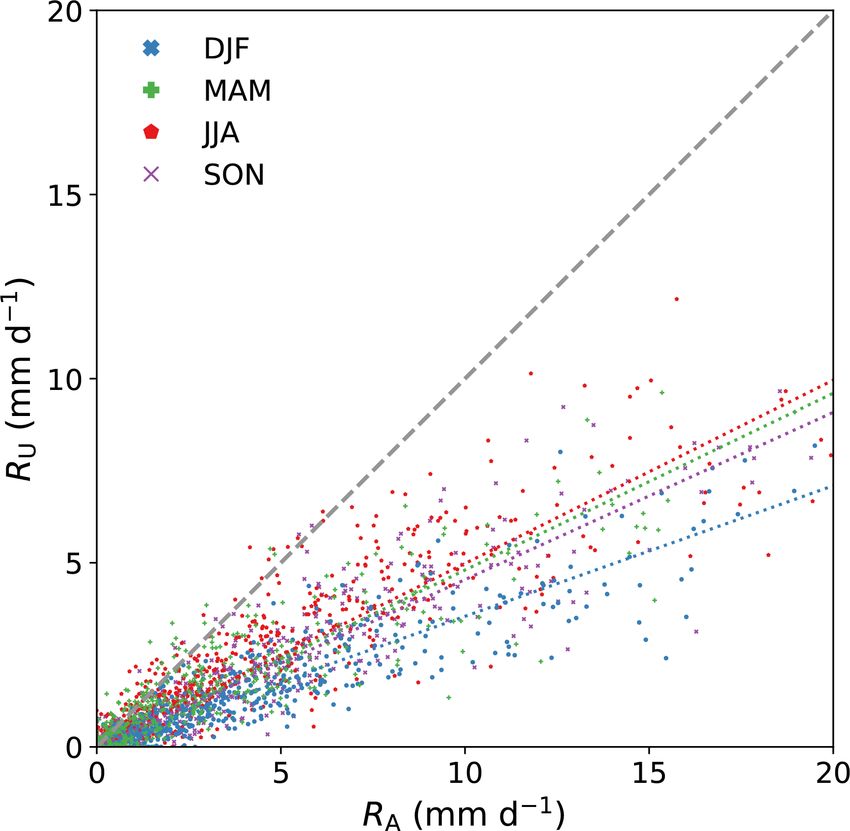
R. Imhoff et al.: A climatological benchmark for operational radar rainfall bias reduction 4067
annual cycle of the adjustment factors, with higher adjust- basins. For all basins, both adjusted products manage to sig-
ment factors from December through March than in the other nificantly increase the QPE towards the reference. However,
months. Figure 4a shows similar results for the catchment- for 9 out of 12 basins, RC outperforms RMFB (Fig. 6e). Ex-
averaged adjustment factors, with factors ranging from 2.1 ceptions are Beemster, Luntersebeek and Dwarsdiep, where
for the Beemster polder to 3.2 for the Hupsel Brook catch- the performance of both products is similar. Differences be-
ment in January, whereas adjustment factors range from 1.3 tween the performance of RC and RMFB become most ap-
for the Grote Waterleiding catchment to 1.6 for the Roggelse- parent for catchments that are located closer to the edges of
beek catchment in June. the radar domain. For instance, RMFB for the Aa and Regge
An explanation for these higher adjustment factors from catchments, which are located in the far south and east of
December through March is that radar QPE often severely the country, still underestimates the annual reference rain-
underestimates the rainfall amounts for stratiform systems, fall sums, with on average 20 % for the Aa (mean annual
which regularly occur during the Dutch winter. This espe- RMFB is 610 mm, and mean annual RA = 761 mm) and 13 %
cially holds when the QPE is constructed from reflectivi- for the Regge (mean annual RMFB is 673 mm, and mean an-
ties sampled above the melting layer (Fabry et al., 1992; nual RA = 776 mm), while this is on average only 5 % (both
Kitchen and Jackson, 1993; Germann and Joss, 2002; Bel- under- and overestimations occur) for RC (Fig. 6b and c).
lon et al., 2005; Hazenberg et al., 2013). This seems to be the The MFB-adjusted QPE performs better for the Beemster
case here as well. A simple first-order estimation of the 0 ◦ C polder, Dwarsdiep polder (Fig. 6d) and Luntersebeek catch-
isotherm level, using a constant wet adiabatic lapse rate of ment (Fig. 6a) due to their location in the radar mosaic. The
5.5 K km−1 with ground temperature data for all rainy hours Luntersebeek catchment (central Netherlands, Fig. 1) is lo-
in the 10 years (Fig. 4b), indicates that the 1500 m pseudo- cated closer to both radars. There, RMFB generally performs
CAPPI is generally above the 0 ◦ C isotherm level from De- better and sometimes even overestimates the true rainfall,
cember through March. This coincides with the months with which is consistent with Holleman (2007). The performance
higher adjustment factors (Fig. 4c) and could thus explain the of RMFB for the Dwarsdiep catchment is similar to its per-
winter effect on the adjustment factors. This effect is presum- formance for the Linde catchment (both in the north of the
ably even stronger further away from the radars because the country), but RC shows more variability in the error from
QPE product consists of samples at even higher altitudes than year to year for the Dwarsdiep catchment (Fig. 6d), leading
1500 m for locations more than 120 km from the radars. Be- to a better relative performance of RMFB . The CARROTS
sides, an additional dependency of the monthly factor on the QPE tends to overestimate the rainfall amount of the three
time of year that cannot be explained by temperature seems aforementioned basins (Beemster, Dwarsdiep and Lunterse-
to be present, with lower adjustment factors during spring beek) for some years (e.g., by 16 % for the Luntersebeek in
and early summer and higher factors for the subsequent pe- 2016). Overall, the performance of RC and RMFB is not that
riod (Fig. 4c). different for these three basins, with on average just a lower
MAE for RMFB than for RC for the Luntersebeek catchment
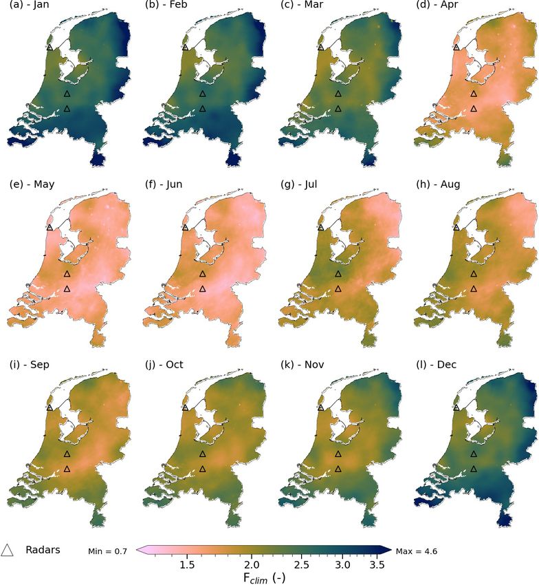
3.2 Evaluation of the rainfall sums and Dwarsdiep polder (Fig. 6e).
Summarizing, the CARROTS factors have a clear an-
The MFB-adjusted QPE (RMFB ) significantly reduces the nual cycle, with generally higher adjustment factors further
systematic bias of RU (Fig. 2), from a 55 % underestimation away from the radars (Sect. 3.1). On average for the Nether-
on average for the Netherlands to 10 % (Fig. 5a and Table 2). lands, the MFB-adjusted QPE outperforms the CARROTS-
However, the remaining bias in RMFB is generally caused by corrected QPE. However, the spatial variability in the CAR-
a systematic underestimation of the reference rainfall. The ROTS factors, in contrast to the uniform MFB adjustment,
overall underestimation is less for RC (8 %, Fig. 5b) but re- results in estimated annual rainfall sums for the 12 hydrolog-
sults from estimation errors that are associated with either ical basins that are generally closer to the reference (for 9 out
under- or overestimates of the reference rainfall. The spread of 12 basins) than with the MFB-adjusted QPE, especially for
in Fig. 5b is significantly wider than in Fig. 5a, indicating the east and south of the country. This effect is expected to
that the country-wide QPE error of RC is often higher than become more pronounced when the adjusted QPE products
for RMFB . The yearly FSE in Table A1 clearly indicates this are used for discharge simulations.
too, with a systematically higher FSE for RC than for RMFB .
An advantage of the MFB adjustment is that it corrects for 3.3 Effect on simulated discharges
the circumstances during that specific day and thus also for
instances with overestimations (Fig. 4a). On a country-wide The severe underestimations of RU have a considerable ef-
level, this is clearly advantageous, also compared to CAR- fect on the discharge simulations for the 12 basins (Fig. 7).
ROTS (Fig. 5). The negative effect of the spatial uniformity This leads to hardly any discharge response and thus nega-
of the factor, however, becomes apparent in Fig. 6, which tive KGE values for most basins as compared to discharge
compares the annual precipitation sums of the two adjusted simulations with the reference rainfall data. The effect is
radar rainfall products with the reference and RU for the 12 most pronounced for the freely draining catchments in the
https://doi.org/10.5194/hess-25-4061-2021 Hydrol. Earth Syst. Sci., 25, 4061–4080, 2021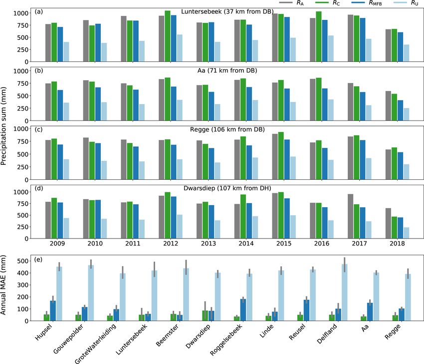
4068                            R. Imhoff et al.: A climatological benchmark for operational radar rainfall bias reduction

Figure 3. Spatial variability of the CARROTS factors, as derived from the archived radar and reference data for the period 2009–2018.
Shown are monthly averages of the daily factors.

east and south of the country. These catchments are more             fall events, leading to higher KGE values (with RU as input)
driven by groundwater flow than the polders in the west of           compared to the other basins.
the country. Groundwater flow gets hardly replenished be-               The model runs using RMFB as input significantly improve
cause of similar estimated annual evapotranspiration and RU          the simulated discharges, compared to the runs with RU .
sums, resulting in baseflows that are too low. The polders, es-      Nevertheless, the model runs still strongly underestimate the
pecially Delfland and Beemster, are an exception to this be-         simulated discharges compared to those from the reference
cause they are less driven by groundwater-fed baseflow and           runs for the catchments in the south and east of the country
more by direct runoff from greenhouses or upward seepage             (Fig. 7a–f). This is particularly noticeable for the catchments
flows, which makes them more responsive to individual rain-          Reusel (KGE = 0.26) and Roggelsebeek (KGE = 0.04). The

Hydrol. Earth Syst. Sci., 25, 4061–4080, 2021                                         https://doi.org/10.5194/hess-25-4061-2021
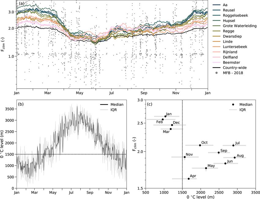
R. Imhoff et al.: A climatological benchmark for operational radar rainfall bias reduction                                                    4069

Figure 4. Seasonal dependency of the CARROTS factors and comparison with the operational MFB-adjustment factor. (a) Temporal vari-
ability of the climatological daily adjustment factors for the 12 basins (colors, catchment-averaged), the country-average (black line) and of
the country-wide hourly MFB factor for the (example) year 2018 (grey dots; some also fall outside the indicated range). (b) Estimate of the
height of the 0 ◦ C isotherm at KNMI station De Bilt for all rainy hours in the 10-year period, based on a constant wet adiabatic lapse rate
of 5.5 K km−1 . (c) Dependency of the monthly adjustment factor on the estimated 0 ◦ C isotherm level for KNMI station De Bilt and the
superimposed grid cell of this station. Depending on the location in the radar composite, the minimum CARROTS factor can take place in a
different month but is always between April and June. Note that for this analysis, the adjustment factor was based on only the rainfall sums
within that month, the “effective adjustment factor” for that month, which roughly coincides with the factor for the 15th of the month in the
CARROTS method. The grey bars indicate the interquartile range (IQR) for that month, based on the spread in hourly 0 ◦ C isotherm level
estimates (the horizontal bars) and the sensitivity to leaving out individual years in the 10-year period for the factor derivation (vertical bars).

spatial uniformity of the MFB factors is identified as the                  age, leading to a more predictable baseflow for all models
cause of these effects because the MFB method can not cor-                  runs. In addition, the catchment is located close to an auto-
rect for the sources of errors leading to the biased QPE in                 matic weather station and is located between both operational
space. This already led to clear underestimations in the an-                radars, which makes the MFB adjustment more beneficial for
nual rainfall sums for these regions (Fig. 6).                              this region. The difference in performance between the hy-
   The CARROTS QPE outperforms RMFB when this prod-                         drological model simulations is small, with a KGE of 0.92
uct is used as input for the 12 rainfall-runoff models. This is             (using RC ) versus 0.96 for RMFB , as compared to the refer-
not exclusively the case for the six catchments in the east and             ence run.
south of the country (Fig. 7a–f), but also for the other polder
and catchment areas. The exception to this is the Beem-
ster polder. The Beemster is mostly fed by upward seep-

https://doi.org/10.5194/hess-25-4061-2021                                                  Hydrol. Earth Syst. Sci., 25, 4061–4080, 2021
4070                               R. Imhoff et al.: A climatological benchmark for operational radar rainfall bias reduction

Table 2. Statistics of Fig. 5. Indicated are the sample size, the Pearson correlation and the slope of a linear fit between the reference and the
two adjusted radar QPE products (RMFB and RC ; the dashed colored lines in Fig. 5). This is indicated per season and for all seasons together
(Total).

                                                              Slope        Pearson correlation           R2
                              Season     Sample size     RMFB         RC   RMFB             RC     RMFB       RC
                              DJF                 902      0.87    0.95      0.99          0.92      0.98     0.85
                              MAM                 920      0.90    0.86      0.99          0.92      0.98     0.85
                              JJA                 920      0.92    0.90      0.99          0.91      0.98     0.83
                              SON                 910      0.90    0.94      0.99          0.93      0.98     0.86
                              Total              3652      0.90    0.92      0.99          0.92      0.98     0.85

Figure 5. Comparison between the reference rainfall (RA ) and the two adjusted radar QPE products: (a) RMFB and (b) RC . Shown are the
daily country-average rainfall sums based on 10 years (2009–2018), classified per season. The slope, Pearson correlation and sample size per
season are indicated in Table 2. The dashed colored lines are a linear fit, forced through the origin, per season between the reference and the
two QPE products.

3.4    Sensitivity analysis                                                sonality in the factor is lost and that an average correction
                                                                           factor remains.
                                                                              In contrast to this, the differences between these six sets of
The use of a different moving window size hardly influences                CARROTS factors (Fig. 8a) lead to minimal variations in the
the CARROTS factors for moving window sizes of 2 weeks                     simulated discharges for the Aa catchment when these fac-
or longer, but this does not hold for moving window sizes                  tors are used to adjust the input QPE (Fig. 8b). Differences
of a day or, to a lesser extent, 1 week (Fig. 8a). The factor              in timing and magnitude (0.2–0.3 mm d−1 ) are visible dur-
derived with a moving window size of 1 d fluctuates heavily                ing peaks and recessions, for instance in early April. How-
from day to day. This suggests that the adjustment factor is               ever, these are small compared to the differences between
still quite sensitive to individual events in the 10-year period,          the model runs with RC and RMFB (Fig. 7). However, the
when a moving window size of 7 d or shorter is used. Moving                use of a window size of 1 d or, to a lesser extent, of a week
window sizes of more than a month (6 weeks and 2 months                    clearly leads to more fluctuations in the CARROTS factor
were tested here) lead to similar CARROTS factors as with                  (Fig. 8a) and can therefore influence the rainfall estimation
a 1-month (31 d) moving window size but somewhat more                      for individual events (and the factor will also be influenced
smoothed. A similar effect likely takes place for a seasonal               by these individual events). For quickly responding catch-
(3-month) moving window. For larger moving window sizes                    ments and urban catchments, this could still lead to different
(half a year to a year, for instance), we expect that the sea-

Hydrol. Earth Syst. Sci., 25, 4061–4080, 2021                                                 https://doi.org/10.5194/hess-25-4061-2021
R. Imhoff et al.: A climatological benchmark for operational radar rainfall bias reduction 4071 Figure 6. Effect of the adjustment factors on the catchment-averaged annual rainfall sums. (a–d) The results for a sample of four catchments that are spread over the country (and thus the radar domain): (a) Luntersebeek, (b) Aa, (c) Regge and (d) Dwarsdiep. Shown are RA (grey), the estimated rainfall sum after correction with the CARROTS factors (RC ; green), the estimated rainfall sum after correction with the MFB- adjustment factors (RMFB ; dark blue) and the rainfall sum with the unadjusted radar rainfall estimates (RU ; light blue). The distance between the catchment center and the closest radar in the domain is given in the title of panels (a–d) (DH is Den Helder and DB is De Bilt). The radar in Herwijnen, which replaced the radar in De Bilt in January 2017, is not included here because this radar was operational for the shortest time in this analysis. (e) The mean absolute error of the annual precipitation sum between the QPE products and the reference rainfall sum (RA ). The vertical grey lines, per bar, indicate the IQR of the mean absolute error (MAE) based on the 10 years. results. In conclusion, a 31 d smoothing of the climatological 4 Discussion adjustment factor is warranted. In addition, leaving individual years out of the 10-year In this study, we introduced the CARROTS method to derive archive has a limited impact on the CARROTS factors (see adjustment factors that reduce the bias in radar rainfall esti- also the vertical bars in Fig. 4c). Similar to the aforemen- mates. We derived these factors using 10 years of 5 min radar tioned results for the moving window size analysis, it leads to and reference rainfall data for the Netherlands. The method hardly any variations in the simulated discharges for the Aa and resulting QPE product outperformed the mean field bias catchment (not shown here). This suggests that the 10-year (MFB) adjustment that is used operationally in the Nether- archive length was sufficiently long for the factor derivation. lands for catchments in the east and south of the country. https://doi.org/10.5194/hess-25-4061-2021 Hydrol. Earth Syst. Sci., 25, 4061–4080, 2021
4072                             R. Imhoff et al.: A climatological benchmark for operational radar rainfall bias reduction

Figure 7. Differences in simulated discharges for the 12 basins (a–l) as a result of the differences between rainfall estimates. The models
are run for the period 2009–2018 with the following rainfall products as input: the reference (RA ; grey), the QPE corrected with the CAR-
ROTS factors (RC ; green), the MFB-adjusted QPE (RMFB ; dark blue) and the unadjusted radar rainfall estimates (RU ; light blue). Only the
simulated discharges for 2015 are shown here for clarity; the KGE is based on all years.

When the QPE products were used as input for hydrological               ence product. According to Saltikoff et al. (2019), at least
model runs, the method outperformed the MFB-adjustment                  40 countries have an archive of historical radar data for a pe-
method for all but one basin.                                           riod of 10 years or more. The proposed CARROTS method is
   The main difference that distinguishes the CARROTS                   potentially valuable for these countries, especially when the
method from the MFB adjustment is the presence of a high-               density of their network of automatic rain gauges is, similar
density network of (manual) rain gauges in the reference                to the Netherlands, significantly smaller than the total net-
dataset, a dataset that is not available in real time. This al-         work of rain gauges. An additional advantage of the method
lows for spatial adjustments. Overeem et al. (2009b) demon-             is the real-time availability of the correction factors, which is
strate that this reference dataset mostly depends on the daily          independent of the timeliness of the rain gauge data.
spatial adjustments from the manual rain gauges, while the                 MFB adjustment of radar rainfall fields is still the most fre-
higher frequency MFB adjustment based on the automatic                  quently applied adjustment method (Holleman, 2007; Harri-
gauges plays a smaller role in the adjustments of this refer-           son et al., 2009; Thorndahl et al., 2014; Goudenhoofdt and

Hydrol. Earth Syst. Sci., 25, 4061–4080, 2021                                             https://doi.org/10.5194/hess-25-4061-2021
R. Imhoff et al.: A climatological benchmark for operational radar rainfall bias reduction                                         4073

Figure 8. Sensitivity of the CARROTS factor derivation to the moving window size. (a) The adjustment factors for the Aa catchment for
six different moving window sizes. The moving window size of 31 d was used in the methodology of this study. (b) The effect of the six
moving window sizes in (a) on the simulated discharges for the Aa. Similar to Fig. 7, the CARROTS factors were derived, and discharge was
simulated for the full period (2009–2018), but only 2015 is shown here. The grey line indicates the observed discharge.

Delobbe, 2016). The results indicate that this choice may              require a recalculation of the adjustment factors, thereby as-
be reconsidered for hydrological applications in the Nether-           suming the presence of an archive of the new composite
lands, especially further away from the radar and in the               product. This could potentially limit the usefulness of the
case that a country-wide or large-region adjustment factor             proposed method. As mentioned in Sect. 2.1, the replacement
is applied. This could also hold for other regions, especially         of both Dutch radars by dual-polarization radars in combina-
mountainous regions, where the uniformity of the MFB-                  tion with the replacement of the radar at location De Bilt by
adjustment factor is likely not sufficient to correct for all          the location Herwijnen (Fig. 1) between September 2016 and
orography-related errors (Borga et al., 2000; Gabella et al.,          January 2017 only had a limited impact on the operational
2000; Anagnostou et al., 2010). More regionalized MFB ad-              products and thereby on the CARROTS derivation. The op-
justments are possible but depend on the density and avail-            erational products are not yet (fully) making use of the dual-
ability of the automatic gauge stations.                               polarization potential. We expect that the factors will have
   However, the proposed CARROTS method has to be recal-               to be recalculated as soon as the additional information from
culated for every change in the radar setup, calibration, addi-        the dual-polarization radars is used to improve the products
tional post-processing steps (e.g., VPR corrections; Hazen-            or when, e.g., the German and Belgian radars close to the
berg et al., 2013) or final composite generation algorithm.            Dutch border are added to the composite.
For instance, including a new radar in the composite would

https://doi.org/10.5194/hess-25-4061-2021                                            Hydrol. Earth Syst. Sci., 25, 4061–4080, 2021
4074                            R. Imhoff et al.: A climatological benchmark for operational radar rainfall bias reduction

   That CARROTS is relatively insensitive to such minor            MFB adjustment (15 % of the cases). Note that for individ-
changes in the composite or the year-to-year variability of        ual events in these 20 extremes, the errors can still reach 48 %
rainfall is likely a result of the 10-year archive that has been   for the QPE adjusted with CARROTS and 64 % for the MFB-
used. The sensitivity analysis in Sect. 3.4 has shown that         adjusted QPE. A way to better correct for biases during ex-
leaving individual years out of the archive hardly influences      treme events could be to derive either different Z–R relation-
the CARROTS factors. Nevertheless, based on the current            ships, depending on the type of rainfall, or dBZ-dependent
analysis, we cannot conclude what the minimum number of            correction factors, which could be derived in a similar way
years in the archive has to be to obtain stable CARROTS fac-       to the CARROTS derivation method. Whether this works or
tors that are similar to the factors derived in this study. This   not for extreme events depends on the number of such events
is a recommendation for future research. In the case of a new      in the available historical dataset.
radar QPE product, it is also recommended to recalculate the          Finally, the CARROTS factors were derived with the ref-
archive (if possible), to make sure new CARROTS factors            erence rainfall data for the Netherlands. The same data were
can be derived.                                                    used as reference in this study. Although the use of the same
   Although the results are promising, this method is not ex-      data as training and validation set is suboptimal, leaving out
pected and meant to outperform more advanced spatial QPE           individual years has had a limited impact on the estimated
adjustment methods, such as geostatistical and Bayesian            adjustment factors and the resulting QPE and discharge sim-
merging methods (for an overview of methods and their lim-         ulations (see also the vertical bars in Fig. 4c). Note, however,
itations, see Ochoa-Rodriguez et al., 2019). A major advan-        that in basins with a large number of manual rain gauges,
tage of these methods is the real-time derivation of spatial       but where automatic rain gauges are not nearby, the CAR-
adjustment factors, in contrast to the proposed method in this     ROTS results will likely be closer to the reference than the
study, which was solely based on historical data. The MFB-         MFB-adjusted simulations. Although this is warranted for
adjustment factors can also be derived in near real time but       the CARROTS method, it can partly explain why the method
are uniform in space, which can explain the worse perfor-          works better for some catchments than others.
mance as compared to the proposed method in this study. A
possible disadvantage of these real-time methods (MFB, geo-
statistical and Bayesian merging) is the dependency on the         5   Conclusions
timely availability of rain gauge data, which is not the case
for CARROTS. Altogether, we consider the proposed clima-           A known issue of radar quantitative precipitation estimations
tological radar rainfall adjustment method to be a benchmark       (QPE) is the significant biases with respect to the true rain-
for the development and testing of operational radar QPE ad-       fall amounts. For this reason, radar QPE adjustments are
justment techniques.                                               needed for operational use in hydrometeorological (forecast-
   Another possible option would be to combine the CAR-            ing) models. Current QPE adjustment methods depend on the
ROTS method with the real-time application of the MFB ad-          timely availability of quality-controlled rain gauge observa-
justment; i.e., CARROTS is applied, and the resulting QPE          tions from dense networks. This especially applies to meth-
is then adjusted with real-time MFB-adjustment factors. This       ods that correct for the spatial variability in the QPE errors.
would allow for real-time temporal corrections of the QPE,         To overcome this issue and to provide a benchmark for fu-
without the need for a high density of rain gauges in real         ture QPE algorithm development, we have presented CAR-
time, while the corrections in space are based on the (histor-     ROTS (Climatology-based Adjustments for Radar Rainfall in
ical) CARROTS factors.                                             an OperaTional Setting), a set of gridded climatological ad-
   As mentioned in the previous paragraph, the climatologi-        justment factors for every day of the year. The factors were
cal adjustment factor is not calculated for the current mete-      based on a historical set of 10 years of 5 min radar rainfall
orological conditions and resulting QPE errors, which could        data and a reference dataset for the Netherlands. The clima-
lead to considerable errors during extreme events. Nonethe-        tological adjustment factors were compared with the mean
less, this is also the case for the MFB-adjustment technique       field bias (MFB) adjustment factors, which are used opera-
(Schleiss et al., 2020). The absolute errors for the 10 high-      tionally in the Netherlands. For the period 2009–2018, daily
est daily sums in this study for the Aa and Hupsel Brook           and sub-daily rainfall estimates with both the MFB-adjusted
catchments (one of the largest and the smallest catchment in       and CARROTS-adjusted QPE were validated against the ref-
the study) are similar for the MFB and climatological ad-          erence rainfall for the land surface area of the Netherlands. In
justment methods, with on average a 20 % difference with           order to provide a hydrometeorological testbed, the estimated
the reference (this would have been 50 % to 60 % without           annual rainfall sums and the effect of the adjusted QPE prod-
corrections). In most of these events, both RC and RMFB un-        ucts on simulated discharges with the rainfall-runoff models
derestimated the true rainfall amount. However, for a small        for 12 Dutch basins were validated for both adjustment meth-
number of these top 10 events, the QPE products overes-            ods.
timated the true rainfall amount. This occurred more fre-             The CARROTS factors show clear spatial and temporal
quently with CARROTS (25 % of the cases) than with the             patterns, with higher adjustment factors towards the edges of

Hydrol. Earth Syst. Sci., 25, 4061–4080, 2021                                       https://doi.org/10.5194/hess-25-4061-2021
R. Imhoff et al.: A climatological benchmark for operational radar rainfall bias reduction                                    4075

the radar domain. This is caused by larger QPE errors further           The main advantage of the introduced method is the con-
away from the radars. The factors are also higher from De-           tinuous availability of spatially distributed adjustment fac-
cember through March than in other seasons. This is likely           tors, due to the independence of timely rain gauge observa-
a result of sampling above the melting layer during these            tions. This is beneficial for operational use. In addition, the
months, which causes higher underestimations in the unad-            CARROTS factors are shown to be robust, as the derivation
justed radar rainfall product.                                       is not found to be sensitive to leaving out individual years or
   On average for the Netherlands, the MFB-adjusted QPE              to the moving window used, especially when this window is
outperforms the CARROTS-corrected QPE. Although the                  longer than a week.
MFB factors are based on the current over- or underestima-              Finally, this method is not expected and meant to outper-
tions in the QPE, the factor is spatially uniform and does not       form more advanced spatial QPE adjustment methods (which
correct for spatial errors. This directly impacts the adjusted       require data from dense rain gauge networks for robust appli-
QPE when the QPE products are tested for the 12 Dutch                cation), but it can serve as a benchmark for the development
basins. The MFB-adjusted QPE leads to annual rainfall sums           and testing of more advanced operational radar QPE adjust-
that still underestimate those of the reference for the catch-       ment techniques. QPE adjustment methods (including CAR-
ments in the east and south of the country (towards the edge         ROTS) greatly benefit from a denser, frequently available
of the radar domain). This bias is almost absent for the annual      rain gauge network. From that perspective, crowd-sourced
rainfall sums after correction with the CARROTS factors (up          personal weather stations have promise for improving radar
to 5 % over- and underestimation for the same catchments).           rainfall products, given their direct surface measurements
For basins closer to radars, this effect decreases, and both         and dense networks (Vos et al., 2019). This also holds for rain
adjustment methods perform well.                                     gauge observations from other governmental or third parties,
   The effects of both adjustment methods on the QPE are             e.g., the water authorities in the Netherlands. Hence, we think
amplified when they are used as input for the rainfall-runoff        that this could further improve radar rainfall products in the
models of the 12 studied basins. The discharge simulations           near future.
with the CARROTS QPE outperform those using the MFB-
adjusted QPE for all but one basin. For hydrological applica-
tions in the Netherlands, these results indicate that the current
operational use of a country-wide MFB adjustment may be
reconsidered as it often performs worse than the proposed
climatological adjustment factor, which can be seen as the
minimum benchmark to outperform.
   Despite the aforementioned results, the CARROTS
method has two main limitations: (1) for every change in the
radar setup, the radar calibration, post-processing algorithms
or the final composite generation method, the adjustment fac-
tors have to be recalculated; (2) the factor is not calculated for
the actual meteorological conditions and resulting QPE er-
rors, which could lead to considerable errors during extreme
events. Nonetheless, the latter is also the case for the MFB-
adjustment technique (Schleiss et al., 2020), even though the
MFB factors are derived in real time.

https://doi.org/10.5194/hess-25-4061-2021                                         Hydrol. Earth Syst. Sci., 25, 4061–4080, 2021
4076                              R. Imhoff et al.: A climatological benchmark for operational radar rainfall bias reduction

Appendix A: Hourly evaluation of the rainfall sums

Table A1. Country-average fractional standard error (FSE) between
the hourly reference rainfall (RA ) and the three QPE products (RU ,
RMFB and RC ) per year for the winter (DJF) and summer (JJA) sea-
sons. The FSE was only calculated for hours in which the country-
average rainfall rate was larger than 0.0 mm h−1 .

                                                 FSE
    Season     Year    Avg. rain rate     RU    RMFB       RC
                          (mm h−1 )
    DJF        2009              0.32    1.10     0.49    0.74
               2010              0.26    1.23     0.61    0.82
               2011              0.38    1.12     0.50    0.73
               2012              0.36    1.09     0.51    0.65
               2013              0.30    1.04     0.56    0.90
               2014              0.33    1.06     0.51    0.72
               2015              0.34    1.04     0.51    0.84
               2016              0.34    1.15     0.61    0.84
               2017              0.37    0.56     0.32    0.44
               2018              0.37    1.22     0.65    0.76
    JJA        2009              0.33    1.18     0.80    1.08
               2010              0.43    1.34     0.71    1.02
               2011              0.37    1.31     0.78    1.03
               2012              0.36    1.19     0.72    0.99
               2013              0.36    1.34     0.86    1.20
               2014              0.33    1.37     0.91    1.28
               2015              0.44    1.24     0.69    1.08
               2016              0.30    1.46     1.00    1.46
               2017              0.37    1.29     0.76    1.09
               2018              0.34    1.26     0.78    1.20

   Table A1 shows the country-average FSE between RA and
the three QPE products for every year and the winter and
summer seasons. The method to calculate the FSE score is
described in Sect. 2.3.

Hydrol. Earth Syst. Sci., 25, 4061–4080, 2021                                     https://doi.org/10.5194/hess-25-4061-2021
You can also read