A single-cell expression simulator guided by gene regulatory networks - bioRxiv
←
→
Page content transcription
If your browser does not render page correctly, please read the page content below
bioRxiv preprint first posted online Jul. 28, 2019; doi: http://dx.doi.org/10.1101/716811. The copyright holder for this preprint (which
       was not peer-reviewed) is the author/funder, who has granted bioRxiv a license to display the preprint in perpetuity.
                                       All rights reserved. No reuse allowed without permission.

      A single-cell expression simulator guided by gene regulatory
      networks

      Payam Dibaeinia1, Saurabh Sinha1,2,3*

      1
        Department of Computer Science, University of Illinois Urbana-Champaign, Urbana, IL, 61801,
      USA
      2
        Carl R. Woese Institute of Genomic Biology, University of Illinois Urbana-Champaign, Urbana,
      IL, 61801, USA
      3
        Cancer Center at Illinois, University of Illinois Urbana-Champaign, Urbana, IL, 61801, USA

      *
       To whom correspondence should be addressed. Tel: 217-333-3233; Email:
      sinhas@illinois.edu

      Abstract
      A common approach to benchmarking of single-cell transcriptomics tools is to generate
      synthetic data sets that resemble experimental data in their statistical properties.
      However, existing single-cell simulators do not incorporate known principles of
      transcription factor-gene regulatory interactions that underlie expression dynamics.
      Here we present SERGIO, a simulator of single-cell gene expression data that models
      the stochastic nature of transcription as well as linear and non-linear influences of
      multiple transcription factors on genes according to a user-provided gene regulatory
      network. SERGIO is capable of simulating any number of cell types in steady-state or
      cells differentiating to multiple fates according to a provided trajectory, reporting both
      unspliced and spliced transcript counts in single-cells. We show that data sets
      generated by SERGIO are comparable with experimental data in terms of multiple
      statistical measures. We also illustrate the use of SERGIO to benchmark several
      popular single-cell analysis tools, including GRN inference methods.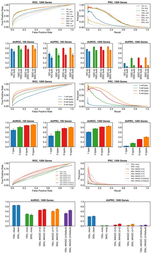
bioRxiv preprint first posted online Jul. 28, 2019; doi: http://dx.doi.org/10.1101/716811. The copyright holder for this preprint (which
       was not peer-reviewed) is the author/funder, who has granted bioRxiv a license to display the preprint in perpetuity.
                                       All rights reserved. No reuse allowed without permission.

      Introduction
      Single-cell transcriptomics technologies are revolutionizing biology today1–4, and have
      led to the rapid development of computational tools for analyzing the resulting data
      sets5–8. These tools, developed for a wide array of tasks such as clustering9–11,
      trajectory inference12,13 and gene regulatory network (GRN) reconstruction9,14,15, as well
      as pre-processing operations such as imputation16–18, adopt complementary strategies
      whose relative merits and weaknesses are not clear a priori. In some cases, single-cell
      data sets annotated using domain knowledge19,20 allow objective evaluations of different
      strategies, but this is not a scalable approach to systematic benchmarking. A promising
      alternative approach is to synthesize single-cell expression data sets that mimic real
      data in their statistical properties and for which underlying biological relationships are
      known by construction.

      Simulation tools (“simulators”) for single-cell expression data have been reported in
      various forms. Several studies offering novel analysis tools use in-house simulators to
      benchmark those tools8,21–26, while other studies specifically develop simulators for use
      by the community27–32. Most of these simulators are geared towards capturing the noise
      characteristics of technologies such as single-cell RNA-seq (scRNA-seq), by first
      estimating statistical quantities describing real data sets and then sampling single-cell
      expression profiles from probability distributions that mirror those quantities. A crucial
      aspect of biology missing in current simulators is the gene regulatory network (GRN):
      the set of transcription factor (TF)-gene relationships that underlies the dynamics and
      steady states of gene expression in each cell. We believe it is imperative that a single-
      cell expression simulator be guided by an underlying GRN, not only because of the
      biological realism that it represents, but also because this is the only direct way to
      benchmark tools specifically designed for GRN reconstruction. Some existing tools do
      attempt to induce gene-gene relationships in synthetic data using multi-gene statistical
      models for sampling purposes28,33, but these attempts do not incorporate the special
      properties of gene regulatory processes that have been reported in the literature34–37,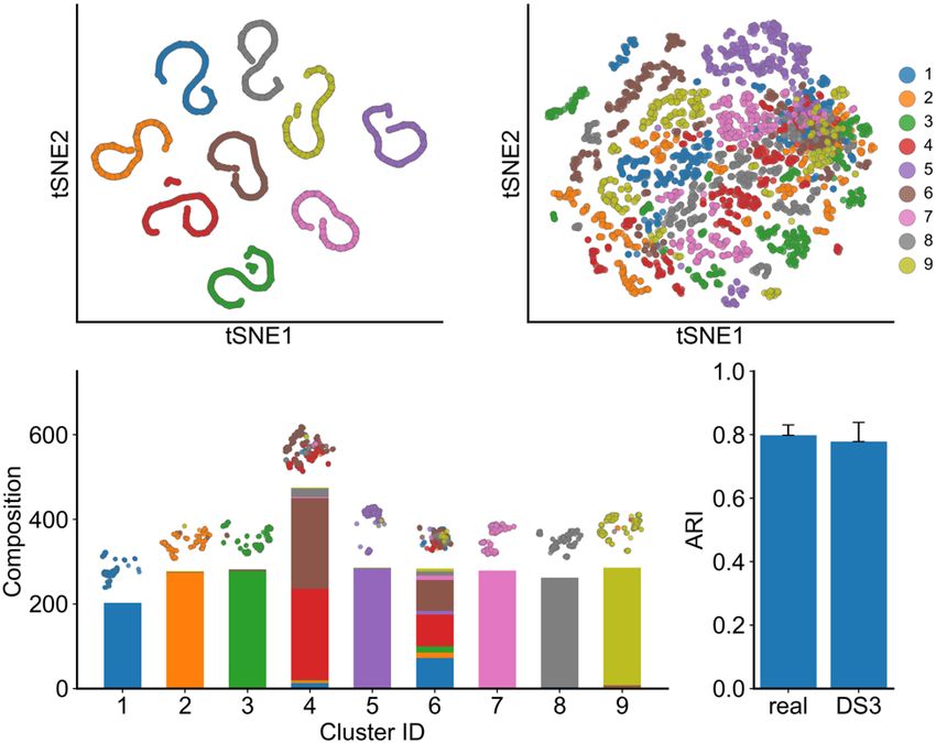
bioRxiv preprint first posted online Jul. 28, 2019; doi: http://dx.doi.org/10.1101/716811. The copyright holder for this preprint (which
       was not peer-reviewed) is the author/funder, who has granted bioRxiv a license to display the preprint in perpetuity.
                                       All rights reserved. No reuse allowed without permission.

      including non-linear response to TFs, intrinsic fluctuations in expression and
      propagation of such “biological noise” along the GRN.

      In the realm of “bulk” transcriptomics GRN-driven simulations are already the norm, as
      exemplified by the simulation tool called GeneNetWeaver (GNW)38, which was used in a
      community-wide effort to benchmark numerous GRN reconstruction tools39–42. GNW is
      not meant to simulate scRNA-seq data, and though some studies have employed
      workarounds to use it for this purpose14,43, it is believed that such synthetic data do not
      exhibit       the statistical characteristics                     of contemporary single-cell                        data sets43.
      Furthermore, such workarounds do not offer key features necessary for a single cell
      expression simulator, such as simulation of multiple cell types and cells differentiating
      from one cell type to another.

      In this work, we develop a simulator tool that (1) uses a principled mathematical
      description of transcriptional regulatory processes to synthesize single-cell expression
      data associated with a specified GRN, (2) includes stochasticity of gene expression as
      an integral part of the process, thus capturing biological noise expected to manifest in
      cell-to-cell variability, and (3) incorporates various types of measurement errors
      (“technical noise”) that are typical of single-cell technologies. The new tool, called
      SERGIO (Single-cell ExpRession of Genes In silico), is freely available as a stand-alone
      software package. It borrows some of its modeling assumptions from the widely used
      GNW simulator, but relinquishes the more complex features of GNW, such as a
      thermodynamics-based model of regulation and explicit modeling of translation
      processes, which would have necessitated use of poorly-understood parameters during
      simulation and slowed down simulations of large GRNs.

      SERGIO uses a stochastic differential equation (SDE) called the chemical Langevin
      equation44 to simulate a gene’s expression dynamics as a function of the changing (or
      fluctuating) levels of its regulators (TFs), as prescribed by a fixed GRN. It performs such
      simulations for any pre-specified number of genes in parallel, and generates single-cell
      expression “profiles” (expression values of all genes) by sampling from these temporal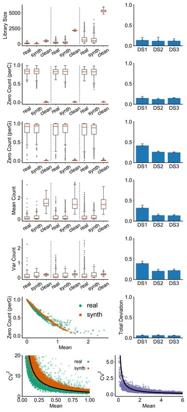
bioRxiv preprint first posted online Jul. 28, 2019; doi: http://dx.doi.org/10.1101/716811. The copyright holder for this preprint (which
       was not peer-reviewed) is the author/funder, who has granted bioRxiv a license to display the preprint in perpetuity.
                                       All rights reserved. No reuse allowed without permission.

      simulations in steady-state, thus mimicking established cell types. It allows users to
      specify the number of cell types to be simulated, via steady-state levels of a few
      “master” regulators in the GRN. SERGIO also allows users to simulate single-cell
      expression data from a specified differentiation program, for which it samples cells from
      transient portions of temporal simulations. In this simulation mode, SERGIO explicitly
      models the splicing step with an additional SDE, resulting in simulations of unspliced
      and spliced transcript levels. SERGIO subjects the synthesized expression data to a
      multi-step transformation where technical noise is incorporated in a manner reflecting
      real scRNA-seq data. To our knowledge, SERGIO is the first stand-alone simulator tool
      for single-cell transcriptomics that offers all of the above-mentioned features while
      basing its simulations on a given GRN. Here, we outline key aspects of its model and
      implementation and show that it may be used to generate realistic data sets that
      resemble an experimental scRNA-seq data set by several statistical measures. We then
      showcase its use to benchmark a number of popular single-cell analysis tools. We find
      that while modern tools are able to accurately identify cell types and differentiation
      trajectories from suitable data sets, their ability to reconstruct gene regulatory
      relationships remains severely limited.

      Results
      We developed SERGIO to simulate how expression values of a specified number of
      genes vary from cell to cell under the control of a given GRN, and how such information
      is captured in modern single-cell RNA-seq data sets. We first simulate “clean” gene
      expression data based on the GRN and mathematical models of transcriptional
      processes, including stochasticity of such processes (“biological noise”). We then add
      “technical noise” to the clean data, mimicking the nature of measurement errors
      attributed to scRNA-seq technology45.

      Simulation of “clean” data
      We generate expression profiles of single cells by sampling them from the steady state
      of a dynamical process that involves genes expressing at rates influenced by other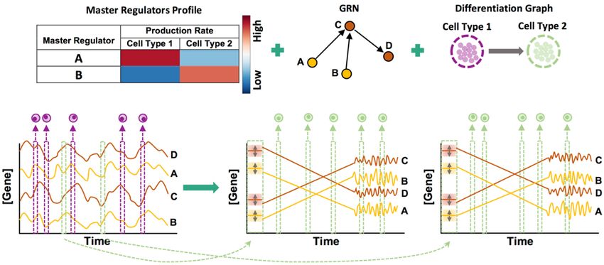
bioRxiv preprint first posted online Jul. 28, 2019; doi: http://dx.doi.org/10.1101/716811. The copyright holder for this preprint (which
       was not peer-reviewed) is the author/funder, who has granted bioRxiv a license to display the preprint in perpetuity.
                                       All rights reserved. No reuse allowed without permission.

      genes (transcription factors) (Figure 1). A select few of the genes are pre-designated as
      master regulators (MRs); these have no regulatory inputs in the GRN and their
      expression evolves over time under constant production and decay rates (see
      Methods). Expression of every other gene (non-MR) evolves under a production rate
      determined by adding contributions from its GRN-specified regulators (equation 5 in
      Methods) and a constant decay rate. Each regulator’s contribution to a gene depends
      on the former’s current concentration and an interaction parameter (strength of
      activation or repression) specific to the regulator and regulated gene. This dependence
      is described by a Hill function46, thus allowing for non-linear effects.

      Each gene’s time course is simulated while incorporating biological noise, using the
      chemical Langevin equation44, as adopted in the GeneNetWeaver (GNW) simulator38.
      Once the system of evolving expression profiles reaches steady state, we sample
      profiles from randomly selected time points. Variation in expression profiles across cells
      of the same type is assumed to mimic variation across time points in the steady state
      (the “ergodic assumption”47), hence the temporally sampled cells are used as the
      collection of cells in the synthetic data.

      Specifying the fixed production rates of MRs determines the average steady state
      expression profile of the sampled cells, and is used to generate data for a single cell
      type. In order to synthesize a data set with multiple cell types, the above simulation is
      repeated using different settings of MR production rates. The aggregate of expression
      profiles sampled across all simulations forms the “clean” synthetic data set.

      Incorporation of technical noise
      We then use the clean data to simulate integer-valued “count” data, as are produced in
      current scRNA-seq technologies, by sampling from a Poisson distribution whose mean
      is the real-valued expression level. However, prior to this conversion, the real-valued
      expression data matrix (genes x cells) is operated upon by modules that incorporate
      three different types of technical noise. The statistical details of these modules are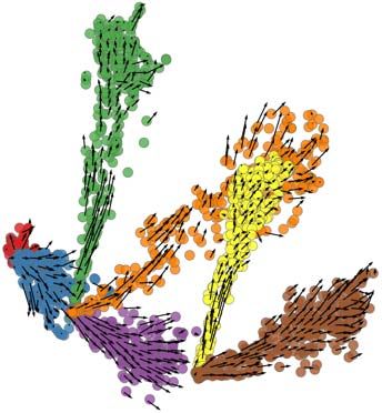
bioRxiv preprint first posted online Jul. 28, 2019; doi: http://dx.doi.org/10.1101/716811. The copyright holder for this preprint (which
       was not peer-reviewed) is the author/funder, who has granted bioRxiv a license to display the preprint in perpetuity.
                                       All rights reserved. No reuse allowed without permission.

      borrowed from the Splatter simulation tool32 and re-implemented in SERGIO (see
      Methods).

      SERGIO simulates realistic data sets
      We used SERGIO to generate synthetic data sets under three different settings of the
      underlying GRN, referred to as “data set 1” (DS1), “data set 2” (DS2) and “data set 3”
      (DS3). These three settings use GRNs with 100, 400 and 1200 genes respectively, that
      were sampled from real regulatory networks in E. coli or S. cerevisae (Table 1); all
      simulations included 300 cells for each of 9 cell types, for a total of 2700 single cells.
      Each data set was synthesized in 15 “replicates” by re-executing SERGIO with identical
      parameters multiple times. We sought to compare statistical properties of these
      synthetic data sets to a published data set from mouse brain comprising expression
      profiles of cells that are categorized into nine cell types with high confidence48,
      henceforth called the “real data set”. We thus configured SERGIO to introduce technical
      noise in the simulated expression profiles, to an extent that matches the real data set.
      This was done through manual iteration of the technical noise parameters (see
      Methods). For each simulation setting we sampled a comparison data set from the real
      data to have the same number of genes, repeating this 50 times to obtain 50 replicates
      of the (sampled) real data set, each of which was compared to the 15 replicates of the
      corresponding synthetic data set. We performed our comparisons using synthetic data
      with and without technical noise, referred to as the “noisy” and “clean” forms of the data
      set.

      We compared several commonly used summary statistics between each synthetic data
      set and a matching real data set (Figure 2). These include two cell-level statistics –
      “library size” and “zero count per cell” (number of genes with zero recorded expression
      in a cell) – and three gene-level statistics – “zero count per gene” (number of cells in
      which a gene has zero recorded expression), “mean count” and “variance count” (mean
      and variance of expression of genes). As shown in Figure 2, there is strong qualitative
      agreement between real and synthetic (noisy) data sets in terms of each of these five
      statistics. As expected, the clean form of each synthetic data set has substantially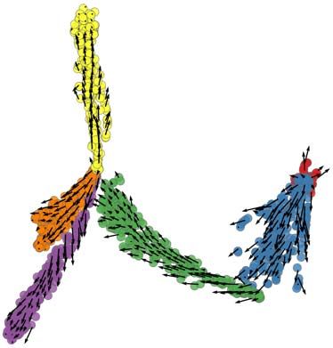
bioRxiv preprint first posted online Jul. 28, 2019; doi: http://dx.doi.org/10.1101/716811. The copyright holder for this preprint (which
       was not peer-reviewed) is the author/funder, who has granted bioRxiv a license to display the preprint in perpetuity.
                                       All rights reserved. No reuse allowed without permission.

      different statistical properties from real data (For a more intuitive interpretation of the
      “total variation” metric used to compare distributions, see Supplementary Figure S2).

      An empirical observation about scRNA-seq data reported in the literature is that there is
      an inverse relationship between the number of zeros in the recorded expression of a
      gene and its mean expression level across cells49,50. This inverse relationship is clearly
      seen in our (noisy) synthetic data sets and their corresponding real data sets (Figure
      2k,l), and arises not only because genes with lower expression levels are more likely to
      result in sampled zero counts, but also because the simulator creates “dropouts” (a form
      of technical noise) with higher probability for such genes. Similarly, an inverse
      relationship between the coefficient of variation (CV) – a common measure of
      expression noise – and mean expression of a gene has been extensively discussed in
      the literature51–53. Figure 2m shows the existence of this relationship in a representative
      synthetic data set as well as in a corresponding real data set. It is not the result of
      adding technical noise, and is present in the clean synthetic data sets as well (Figure
      2n). It arises naturally from the gene regulatory model implemented in SERGIO, in
      contrast to other single cell simulators that explicitly add such a relationship to their
      statistical sampling procedures32. In other words, the synthetic data sets generated by
      SERGIO not only exhibit realistic distributions of key summary statistics (Figure 2a-j),
      they also exhibit second-order relationships between pairs of variables that are
      characteristic of real data sets (Figure 2k-n).

      Simulated data exhibit cell heterogeneity similar to real data
      Motivated by the growing use of single cell RNA-seq data to characterize cellular
      heterogeneity in biological samples, we next asked if the synthetic data sets from
      SERGIO exhibit heterogeneity similar to real ones. We first used Principal Components
      Analysis (PCA) to reduce each cell’s representation to 10 dimensions and then used the
      popular tSNE algorithm to plot cells in two dimensions. Figures 3a and 3b show such
      tSNE plots for a representative synthetic data set (in the DS3 setting) in their clean and
      noisy forms respectively. It is clear that in the absence of technical noise the nine cell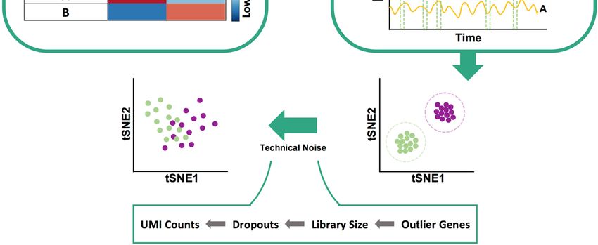
bioRxiv preprint first posted online Jul. 28, 2019; doi: http://dx.doi.org/10.1101/716811. The copyright holder for this preprint (which
       was not peer-reviewed) is the author/funder, who has granted bioRxiv a license to display the preprint in perpetuity.
                                       All rights reserved. No reuse allowed without permission.

      types (as specified during simulation) are highly distinguishable, and that the noisy data
      sets smear this visual separability significantly.

      However, cell type detection in practice does not rely only on visual separation, and
      specialized high-dimensional clustering algorithms are being developed for the purpose.
      One such algorithm is SC311, which has been shown to have high accuracy for the task.
      It was used by Aibar et al.9 to cluster mouse cortex cells in the “real data set” of our
      study48 and the clusters were found to be very similar to the true cell types present in
      the sample (Adjusted Rand Index, ARI, of ~0.8). If our synthetic data sets exhibit similar
      levels of cellular heterogeneity as the real set, then we expect SC3-reported clusters to
      have similar levels of concordance with “true” cell types as known to the simulator.
      Figure 3c shows the composition of nine clusters found by SC3 on the (noisy) synthetic
      data set visualized in Figure 3b, in terms of the true cell types present in each cluster.
      We note that seven of the nine reported clusters predominantly comprise cells of one
      (distinct) type, and only two of the clusters are of mixed composition, thus suggesting a
      high accuracy of clustering. To make this observation more formal, we computed the
      Adjusted Rand Index (ARI) between SC3-reported clusters and true cell types for each
      of the 15 replicates of the DS3 data set, noting an average ARI of 0.78. We repeated
      this for each of the 50 sampled subsets of the real data set corresponding to DS3
      settings, and found the average ARI to be 0.80, very close to that seen in synthetic
      data. This exercise demonstrates that synthetic data sets generated by SERGIO exhibit
      realistic levels of cellular heterogeneity also illustrates the use of SERGIO to benchmark
      clustering methods.

      Benchmarking GRN reconstruction methods
      We next illustrate how the data synthetized by SERGIO can serve to benchmark GRN
      reconstruction tools. In our first tests we worked with clean data sets generated by
      SERGIO, reasoning that these should provide an upper bound for performance on noisy
      realistic data sets. We evaluated the popular GRN inference algorithm called GENIE354,
      which was originally developed for analyzing bulk RNA-seq data but has since been
      used successfully on single cell data as well. We applied GENIE3 on the (clean) data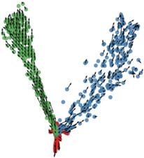
bioRxiv preprint first posted online Jul. 28, 2019; doi: http://dx.doi.org/10.1101/716811. The copyright holder for this preprint (which
       was not peer-reviewed) is the author/funder, who has granted bioRxiv a license to display the preprint in perpetuity.
                                       All rights reserved. No reuse allowed without permission.

      sets DS1 (100 genes) and DS3 (1200 genes) and evaluated the predicted TF-gene
      pairs based on the underlying GRNs in these data sets, using the common metrics Area
      Under Receiver Operating Characteristics (AUROC) and Area Under Precision-Recall
      Curve (AUPRC). Recall that these data sets were synthesized to include 300 cells for
      each of nine cell types. To assess the impact of data set size, we created smaller sets
      by sampling 200, 100 or 10 cells per cell type from the original simulated data (for each
      replicate of DS1 and DS3), and repeated the GRN reconstruction assessments for
      these. We also sought to assess the advantage of having single cell resolution in the
      data, and thus synthesized “bulk” expression data sets by averaging the expression of
      each gene in all cells of the same type, mimicking a situation where each cell type has
      been sorted separately and subjected to traditional expression profiling. (The resulting
      synthetic data sets included nine conditions with “bulk” expression values of each of 100
      or 1200 genes, depending on the original data set.)

      Figures 4a and 4b show the ROC and PRC respectively for a representative replicate of
      the DS3 data set, in its original setting (300 cells per type) as well as its sampled
      smaller versions and their respective “bulk” data set versions. A more comprehensive
      view, spanning all replicates of DS1 and DS3, is shown in Figure 4c-f. Several points
      are apparent from these figures. First, in nearly all versions of the data sets, GENIE3
      performs significantly better than random, as is evident from AUROC values well above
      the 0.5 value expected from a random predictor. Second, we note that while
      performance is significantly better on larger data sets than on the smallest data set (10
      cells per type), there is not a clear difference among the data sets with 100 cells per
      type or more. This suggests that, at least in the absence of technical noise, the benefits
      of greater cell count for GRN reconstruction accuracy saturate at commonly seen levels.
      Third, the “bulk” data sets consistently yielded lower accuracy than the single-cell data
      sets, regardless of the numbers of cells, confirming the value of the latter for regulatory
      inference. Finally, we noted that although the DS1 and DS3 data sets had similar
      AUROC values, the AUPRC values revealed significantly worse predictions in the larger
      (DS3, 1200 genes) data sets. This is expected, in part because the random baseline is
      lower for DS3 (random AUPRC of 0.002) than for DS1 (random AUPRC of 0.026), but
bioRxiv preprint first posted online Jul. 28, 2019; doi: http://dx.doi.org/10.1101/716811. The copyright holder for this preprint (which
was not peer-reviewed) is the author/funder, who has granted bioRxiv a license to display the preprint in perpetuity.
All rights reserved. No reuse allowed without permission.
also because high levels of gene co-expression confound methods such as GENIE3
more for larger data sets.
We next examined the impact of cellular heterogeneity on GRN reconstruction
accuracy, using our clean synthetic data sets. For this, we sampled from each replicate
of DS1 and DS3 (at their original setting of 300 cells per type) smaller data sets
comprising 6, 3 or 1 cell type rather than the 9 cell types simulated. As shown via
AUROC and AUPRC measures in Figures 4i-l (with representative ROC and PRC
curves in Figures 4g,h), we found data sets with greater heterogeneity to consistently
improve GENIE3 performance, which remained clearly above the random baseline
(AUROC of 0.5 and AUPRC of 0.026 and 0.002 for DS1 and DS3 respectively) for all
but the “1 cell type” setting. This is expected, since the latter setting includes gene
expression variation resulting only from biological noise, and even though extrinsic
noise (fluctuations in TF levels reflected in target gene levels55) may be exploited to
infer TF-gene relationships, such correlations are diluted by the presence of intrinsic
gene expression noise in the simulations (see Methods). On the other hand, in settings
with 3 – 9 different cell types, the dominant form of expression variation arises from
differences in the steady state profiles of the cell types, making regulatory inferences
more effective.
We next examined the effect of technical noise on GRN reconstruction. For this, we
compared GENIE3 performance on clean and noisy versions of each replicate of DS3
(1200 genes), in the original setting of 300 cells per type as well as a sampled version
thereof with 100 cells per type. The complete results are shown in Figures 4o,p, with
representative ROC and PRC curves shown in Figures 4m,n. Both performance metrics
(AUROC and AUPRC) deteriorate to levels expected from random prediction when
analyzing noisy synthetic data, in contrast to the very high levels seen prior to
introducing technical noise. Such nearly-random performance of GENIE3 on noisy
single-cell expression data has been reported in previous studies conducted based on
real as well as synthetic single-cell expression data sets43,56. Notably, increasing the
number of cells (from 100 per type to 300) does not change our conclusion.bioRxiv preprint first posted online Jul. 28, 2019; doi: http://dx.doi.org/10.1101/716811. The copyright holder for this preprint (which
was not peer-reviewed) is the author/funder, who has granted bioRxiv a license to display the preprint in perpetuity.
All rights reserved. No reuse allowed without permission.
In light of the above finding, we considered the possibility of using imputation tools
specialized for single cell RNA-seq data as a means to improve the signal necessary for
GRN reconstruction. We thus utilized the popular imputation tool called MAGIC17 to pre-
process the noisy synthetic data sets prior to analyzing them with GENIE3, and
compared the performance metrics to those obtained above. Results were only
modestly improved from those without imputation, with AUROC values ~ 0.65 in the 300
cell/type setting and ~ 0.52 in the 100 cell/type setting (Figures 4m-p). Closer
examination revealed that the default settings of MAGIC made the data overly
structured, resulting in unrealistically large gene-gene correlations (Supplementary
Figures S3 and S4), similar to previous reports57–59. In order to address this issue, we
employed two smaller values of the ‘t’ parameter in MAGIC (t = 2 or 7), in separate runs,
prior to GRN reconstruction. Both of these settings resulted in improved performance
over the default setting of MAGIC, and substantially better than that seen in noisy data
sets without imputation (Figures 4m-p). For instance, AUROC values for the 300
cell/type setting were at ~0.70 (t = 7), squarely in the middle of those without imputation
(~0.46) and those on clean data sets (~0.86). AUPRC values (~0.08) were also
significantly above random expectation (~0.002), though far from the high values ~0.4
observed on clean data sets. Although we noted above that GRN reconstruction
accuracy on clean data sets did not improve when increasing the cell counts (300
versus 100 cells per type), we do notice a significant and consistent effect of cell counts
in performance on imputed data (Figures 4o,p). Presumably, greater cell counts are
beneficial for the imputation step, which in turn results in higher performance of
GENIE3. Our overall conclusion from the above tests (Figure 4) is that a state-of-the-art
GRN reconstruction method such as GENIE354 can perform accurately on single cell
expression data in the hypothetical scenario where technical noise is absent, but falls to
near-random performance in the face of realistic levels of technical noise. The accuracy
does improve above random baseline if the data are imputed with specialized tools but
remains far short from the upper bar observed in clean data, making technical noise a
major factor for future GRN reconstruction methods to address.bioRxiv preprint first posted online Jul. 28, 2019; doi: http://dx.doi.org/10.1101/716811. The copyright holder for this preprint (which
was not peer-reviewed) is the author/funder, who has granted bioRxiv a license to display the preprint in perpetuity.
All rights reserved. No reuse allowed without permission.
Benchmarking differentiation trajectory inference tools
Our analysis so far involved using SERGIO to synthesize steady-state expression
profiles representing different cell types. The simulator is additionally capable of
synthesizing dynamic expression data on a set of genes controlled by a given regulatory
network in single cells differentiating along a given trajectory (Figure 5). In this mode the
simulator is provided with a differentiation graph whose nodes represent stable cell
types in a differentiation program and whose edges represent differentiation from the
parent cell type to child cell type. The simulator samples expression profiles from the
steady state represented by the parent cell type, and then simulates a dynamical
process (identical to that described above) that begins with one of these expression
profiles and evolves into the steady state represented by the child cell type. It then
samples expression profiles from the temporal duration when the cells are transitioning
from the initial to final cell type. The entire “clean” data set is synthesized by repeating
this simulation process for each edge in the differentiation graph. Technical noise is
then added in a manner identical to the steady state simulation mode.
An emerging approach to describe the dynamics of differentiation programs through
single-cell expression profiling involves examination of spliced as well as unspliced
transcript levels in the data and inferring “RNA velocity” of each gene60. To allow
synthesizing data sets amenable to such analysis, the differentiation simulation mode
uses a variation on the underlying model described above. In particular, it invokes two
chemical Langevin equations (CLE) similar to equation 1 to generate unspliced and
spliced transcript levels (see Equation 8 and 9 in Methods). It reports the simulated
expression values as levels of unspliced as well as spliced transcripts, whose sum may
be considered the total expression of a gene.
To illustrate these features of the simulator, we generated four synthetic differentiation
data sets (DS4 – DS7), each containing 100 genes controlled by the same GRN, but
obeying different differentiation graphs – linear (DS4), bifurcation (DS5), trifurcation
(DS6) and tree (DS7) (Figure 6, top). Figure 6a shows the two dimensional PCA plot of
the clean total transcriptome (without technical noise added) for the four types ofbioRxiv preprint first posted online Jul. 28, 2019; doi: http://dx.doi.org/10.1101/716811. The copyright holder for this preprint (which
was not peer-reviewed) is the author/funder, who has granted bioRxiv a license to display the preprint in perpetuity.
All rights reserved. No reuse allowed without permission.
differentiation graphs. It is visually evident that these two-dimensional representations of
cells based on their gene expression profiles match their corresponding graphs used in
the simulations. We note that the dispersion of cells of each type (end points of each
branch of a graph) as well as the width of the differentiation path from one type to
another can be controlled by user-specified parameters in SERGIO (Supplementary
Figure S5).
Differentiation data sets synthesized by SERGIO can be used to benchmark trajectory
inference algorithms since the underlying differentiation trajectory (graph) is known for
these data. To illustrate this, we applied the Slingshot13 tool on the above data sets, still
in their clean form without technical noise. Slingshot is a tool specifically developed for
trajectory inference, with published reports of high accuracy. Consistent with these
reports, we noted that Slingshot infers the correct trajectory in three of the four data
sets; however, it failed to reconstruct the more complex, tree trajectory (Figure 6b) of
DS7.
We then analyzed the above synthetic data sets with the Velocyto60 tool, which infers an
“RNA velocity” field in a low dimensional representation of single cells that indicates the
direction in which each cell’s expression profile appears to be changing. The velocity
field also provides an intuitive visualization of differentiation trajectories. Figures 6c,d
depict the inferred velocity fields for DS6 and DS7, demonstrating how Velocyto
correctly captures these differentiation trajectories, including the tree of DS7 (Figure 6d)
that Slingshot was unable to recover (Figure 6b, right). (Velocyto output for DS4 and
DS5 may be found in Supplementary Figure S6.) Thus, we find that use of an additional
layer of information – spliced versus unspliced mRNA counts – can improve trajectory
inference from single cell transcriptomic data. This is not limited to data sets with
complex underlying trajectories – Figure 6e shows an example data set (DS8)
generated using a simple bifurcation graph for which Slingshot infers a linear trajectory
while Velocyto reports a velocity field clearly indicative of the true bifurcation trajectory.
It is worth noting here that the Slingshot tool may be made to utilize prior knowledge of
stable cell types, and we did not provide such information, which may resolve the errorsbioRxiv preprint first posted online Jul. 28, 2019; doi: http://dx.doi.org/10.1101/716811. The copyright holder for this preprint (which
was not peer-reviewed) is the author/funder, who has granted bioRxiv a license to display the preprint in perpetuity.
All rights reserved. No reuse allowed without permission.
noted above. To summarize, synthetic data sets generated by SERGIO show that, at
least in the absence of prior information on stable cell types, RNA velocity-based
approaches may have an advantage in terms of trajectory inference on single cell data.
Benchmarking GRN reconstruction on differentiation data
Single-cell transcriptomic profiles of differentiation processes offer unique opportunities
for GRN reconstruction, where cells are ordered by “pseudotime” (a temporal partial
ordering obtained by mapping them to inferred differentiation paths) and the resulting
pseudotime labels are exploited to infer causal relationships between TFs and target
genes. Several methods have been recently proposed that specifically channel this
opportunity, including SCODE56, SINCERITIES61 and SINGE62. We used the dynamic
data simulated by SERGIO to benchmark these specialized GRN-reconstruction
algorithms, using Slingshot for pseudotime inference. We used one simulated replicate
of DS4, DS5 and DS6, for which we verified above that Slingshot infers trajectories
accurately. For each data set, we evaluated and compared the three above-mentioned
GRN reconstruction methods on single cells associated with a single branch of the
inferred differentiation trajectory (see Methods). We also used GENIE3 as a baseline
method to infer TF-gene relationships without utilizing pseudotime information.
Interestingly, GENIE3 clearly outperforms the three specialized algorithms in all six
evaluations (Figure 6f,g). In other words, the use of temporal ordering of single cells
does not help GRN reconstruction, at least in the absence of technical noise.
Discussion
The main distinguishing quality of SERGIO is its ability to simulate single-cell
expression data based on a specified GRN. Its implementation strikes a balance
between a biologically realistic model of transcriptional processes and simplifying
assumptions that facilitate fast simulation, capable of scaling to thousands of genes and
regulatory interactions. SERGIO employs an intuitive definition of cell types as steady
states of GRN dynamics63, and can simulate any number of user-defined cell types. It
can also simulate collections of cells differentiating from one cell type to another, anbioRxiv preprint first posted online Jul. 28, 2019; doi: http://dx.doi.org/10.1101/716811. The copyright holder for this preprint (which
was not peer-reviewed) is the author/funder, who has granted bioRxiv a license to display the preprint in perpetuity.
All rights reserved. No reuse allowed without permission.
important feature not available in GNW 38 even after modifications to simulate single-cell
data. Additionally, by including separate simulation of unspliced and spliced transcripts
in differentiating cells, SERGIO allows assessment of tools based on the emerging
approach of RNA velocity.
The unique features of SERGIO make it a powerful tool for benchmarking a wide variety
of single-cell analysis tools. We have presented several examples of such
benchmarking efforts, which yielded useful insights about the evaluated tools. For
instance, we showed a simple example (Figure 6e) of a differentiation data set where
RNA velocity-based inference outperforms alternative trajectory inference algorithms.
Our assessment of a leading GRN inference tool found that it is rendered largely
inaccurate (close to random performance) due to technical noise typical of
contemporary data sets, even though they are capable of far greater accuracy in the
absence of measurement errors. In the same context, we noted that imputation
algorithms such as MAGIC17 can alleviate this problem to an extent, leading to modestly
improved accuracy, especially if data sets have larger numbers of cells.
We also evaluated GRN inference methods designed specifically for time-ordered
single-cell expression data56,61,62, and were surprised to find that these specialized
methods are less effective than a more general-purpose method – GENIE354 – even for
differentiation data sets. However, the performance of these specialized tools depends
on the type of differentiation trajectories, number of single-cells and other factors. For
example, SINGE62, one of the evaluated methods, is designed to be used with an
ensemble of parameter settings, and in our evaluations we used this tool with only two
sets of parameters; its performance might have been significantly better if a larger
ensemble of parameters were to be used.
It should be noted that the GRN benchmarking in this study considered methods based
on expression only, while better accuracy can result from existing tools that use
additional information such as TF-DNA binding data9. Future work can combine
SERGIO simulations of single-cell expression with existing ideas on benchmarking GRNbioRxiv preprint first posted online Jul. 28, 2019; doi: http://dx.doi.org/10.1101/716811. The copyright holder for this preprint (which
was not peer-reviewed) is the author/funder, who has granted bioRxiv a license to display the preprint in perpetuity.
All rights reserved. No reuse allowed without permission.
inference from bulk data and prior information64. Expression data from TF knockout
experiments can also be exploited by GRN inference algorithms65, and knockout of
master regulators (MR) can be easily simulated in SERGIO to assess such algorithms.
In conclusion, we believe that SERGIO will prove useful to a number of researchers
developing tools for the rapidly developing field of single-cell transcriptomics. It will be
especially useful for testing GRN reconstruction methods, which according to our
assessments is the analytical task most in need of future improvements. But its
usefulness will extend to future tools for other popular tasks as well, since synthetic data
sets that capture real data more closely naturally provide more reliable assessments of
those tools. Moreover, the “clean” simulated data sets (without technical noise)
generated by SERGIO should be useful in their own right, since they also capture
realistic expression variation due to biological noise and can provide upper bounds on
accuracy in the idealized scenario where measurement noise has been eliminated.
Methods
Steady-State Simulations
We model the dynamics of the concentration of genes using systems of stochastic
differential equations (SDE) that have been previously employed in GeneNetWeaver
(GNW)38,40 and which are derived from the chemical Langevin equation (CLE)44. The
time-course of mRNA concentration of gene i is modeled by:
(1)
where is the expression of gene i, is its production rate, which reflects the influence
of its regulators as identified by the given GRN (details below), is the decay rate, and
is the noise amplitude in the transcription of gene i. and are two independent
Gaussian white noise processes. In order to obtain the mRNA concentrations as a
function of time, we integrate the above stochastic differential equation for all genes:bioRxiv preprint first posted online Jul. 28, 2019; doi: http://dx.doi.org/10.1101/716811. The copyright holder for this preprint (which
was not peer-reviewed) is the author/funder, who has granted bioRxiv a license to display the preprint in perpetuity.
All rights reserved. No reuse allowed without permission.
బ
బ బ
(2)
బ
where and are two independent stochastic Wiener processes. We integrate this
equation in pre-defined time steps of duration , according to Euler–Maruyama
method66 using the Itô scheme:
(3)
~ √ 0,1 , ~ √ 0,1 (4)
Each iteration yields the mRNA concentrations of all genes at time step Δ using
each gene’s own concentration and all of its regulators’ concentrations at time step .
We model each gene’s production rate, , as the sum of contributions from each of its
regulators (as prescribed by the GRN):
(5)
where ! is the set of all regulators of gene i, is the basal production rate of gene i,
and is the regulatory effect of gene (TF) j on gene i. The latter is modeled as a non-
linear saturating Hill function of the mRNA concentration of the TF46:
ೕ
ೕ
" ೕ ೕ ; if regulator j is an activator of gene i (6)
ೕ ೕ
ೕ
ೕ
" 1 ೕ ೕ ; if regulator j is a repressor of gene i (7)
ೕ ೕbioRxiv preprint first posted online Jul. 28, 2019; doi: http://dx.doi.org/10.1101/716811. The copyright holder for this preprint (which
was not peer-reviewed) is the author/funder, who has granted bioRxiv a license to display the preprint in perpetuity.
All rights reserved. No reuse allowed without permission.
where " denotes the maximum contribution of regulator j to target gene i, # is the Hill
coefficient that introduces non-linearity to the model and $ is the regulator
concentration that produces half-maximal regulatory effect (half-response). If gene i is a
user-designated “master regulator” (MR), i.e., no gene regulates it, then its production
rate is entirely determined by basal production rate which is a user-defined
parameter. For simplicity, we set 0 for genes other than master regulators. " and
# are user-defined parameters, and the type of each interaction (activation or
repression) is also user-specified. The $ parameter is set to be the average of the
regulators’ expression among the cell types to be simulated. The parameters and in
equation 1 characterize the intrinsic noise associated with the production and decay
processes of the mRNA transcript of gene i. Moreover, the intrinsic noise in the
transcription of regulators propagates along the GRN and thus influences the production
rate to become an extrinsic noise source in the transcription of gene i. We support
three forms of noise:
1. Dual Production Decay (“dpd”): the form of stochastic noise that is shown in
equation 1.
2. Single Production (“sp”): including only the noise term associated with the
production process (equivalently, set 0).
3. Single Decay (“sd”): including only the noise term associated with the decay
process (equivalently, set 0)
We note that the current version of Sergio is not capable of simulating GRNs containing
auto-regulatory edges or cycles.
Sampling Single Cells
We use the above system of equations to simulate the time-course of each gene’s
expression in a cell, starting with a given initial value, and record expression values of
all genes at randomly selected time points after the simulation has reached steady
state. Invoking the ergodic assumption47, we treat the expression profiles at these time
points to represent single-cell profiles. In order to speed up the simulation, we estimatebioRxiv preprint first posted online Jul. 28, 2019; doi: http://dx.doi.org/10.1101/716811. The copyright holder for this preprint (which
was not peer-reviewed) is the author/funder, who has granted bioRxiv a license to display the preprint in perpetuity.
All rights reserved. No reuse allowed without permission.
the steady-state concentrations of all genes given the input parameters (see
Supplementary Notes 1) and initialize the time-course simulation with those values.
Also, we ensure that a sufficient number of time steps, which is controlled by a user-
defined parameter, are simulated in the steady state prior to sampling cells.
Cell Types
The above simulation is performed for each “cell type” separately. We define a cell type
(or cell state) by the average concentration of master regulators. A cell type differs from
another cell type by the average concentration of one or more of the master regulators
among the population of cells belong to each cell type. This can be controlled by the
basal production rate b for master regulators (see Supplementary Notes 1). Sergio
takes as input the basal production rate of all master regulators in each of the cell types
to be simulated.
Simulation of differentiation trajectories
In addition to simulating one or more “cell types” in steady state, Sergio may be used to
simulate cells on the differentiation trajectory from one cell type to another, i.e., between
two steady states. More generally, given a “differentiation graph” where nodes represent
cell types and directed edges indicate differentiation from one cell type to the other,
Sergio can simulate expression profiles of cells spanning different stages of
differentiation specified by the graph. Such cells are either in one of the steady states
represented by nodes or have departed away from the steady-state of their “parent” cell
type of an edge and are migrating toward the steady-state of the corresponding “child”
cell type. The differentiation is presumed to commence when one or more master
regulators change their expression from that in the steady state of the parent cell type,
e.g., due to a signaling event67 or due to a noise-driven switch68. Thus, given a
differentiation graph and average expression levels of master regulators for each cell
type (nodes), we simulate each differentiation trajectory (edge) as follows: 1) Cells
representing the parent cell type are sampled from the corresponding steady state. 2)
Production rates (Pi) of master regulators are changed from those specified for the
parent cell type to those of the child cell type, and time-course simulations arebioRxiv preprint first posted online Jul. 28, 2019; doi: http://dx.doi.org/10.1101/716811. The copyright holder for this preprint (which
was not peer-reviewed) is the author/funder, who has granted bioRxiv a license to display the preprint in perpetuity.
All rights reserved. No reuse allowed without permission.
performed following equations 3-4 as explained above. As these simulations proceed,
all genes ultimately converge to their steady-state concentrations in the child cell type.
3) Cells (expression profiles) are sampled at random from the entire simulation,
including cells in the parent and child cell types (steady states) as well as cells on the
differentiation trajectory (transient states). Multiple such time-course simulations are
performed and the sampled cells are randomly chosen from the entire collection of such
simulations. Also, after each simulation reaches the steady-state of the child cell type, it
may be continued for a user-defined number of additional steps. This controls the ratio
of the cells in the steady states of the differentiation graph to the number of cells in
differentiating (transient) states.
Simulations of differentiation trajectories in Sergio generate not only the total mRNA
concentration of each gene (in a time-course), but the changing levels of spliced and
unspliced mRNA transcripts separately. To this end, we express the rate of change in
the concentration of unspliced and spliced RNA using ordinary differential equations
(ODEs), following prior work60,69. Furthermore, we introduce noise terms to these ODEs
in a manner similar to steady-state simulations (equation 1). Thus, the time-course of
the spliced (s) and unspliced (u) transcript level of gene i is modeled as:
%
& % & % (8)
'
& % ( '
& % ) ( ' * (9)
where is the production rate of pre-mRNA (unspliced transcript) that includes
regulatory interactions, and & are the degradation and splicing rate respectively of
pre-mRNA and is the noise amplitude associated with the transcription of pre-mRNA.
For simplicity, we assume the degradation rate of pre-mRNA is zero and all of its
decay is due to splicing (user-defined parameter & ). Also, ( is the degradation rate of
spliced mRNA and is the noise amplitude associated with the transcription of spliced
mRNA. , , ) and * are independent Gaussian white noise processes. All the three
form of stochastic noise (“dpd”, “sp”, “sd”) described for steady-state simulations arebioRxiv preprint first posted online Jul. 28, 2019; doi: http://dx.doi.org/10.1101/716811. The copyright holder for this preprint (which
was not peer-reviewed) is the author/funder, who has granted bioRxiv a license to display the preprint in perpetuity.
All rights reserved. No reuse allowed without permission.
also supported in dynamics simulation. Moreover, production-rate is modeled as in
steady-state simulations (equations 5-7 above). Both of the SDEs in equations 8-9 are
integrated according to Euler–Maruyama scheme to obtain time-courses of unspliced
and spliced mRNA concentrations.
Technical Noise
Sergio adopts methods similar to Splatter32 for adding technical noise to the simulated
single-cell expression data. One module introduces the phenomenon of “outlier genes”,
which refers to the empirical observation that a small set of genes appear to have
unusually high expression measurements across cells in typical scRNA-seq data sets. A
second module incorporates the noted phenomenon of different cells having different
total counts (library size), that follows a log-normal distribution. A third module
introduces “dropouts”, which refers to the observation that a high percentage of genes
are recorded at zero expression in any given cell, indicating an experimental failure to
record their expression rather than true non-expression. These three modules may be
invoked optionally and in any combination and order specified by the user. We
elaborate on each of these modules below. We focus on details pertinent to simulation
of steady state data; corresponding details for differentiation trajectory data are provided
in Supplementary Notes 3. Each of the modules outlined below adds a single type of
technical noise to the data set provided to it.
Outlier genes: Each gene is designated as an outlier with a user-defined probability. If
so, its expression (in every cell) is multiplied by a factor sampled from a log-normal
distribution, otherwise the expression is left unchanged:
+, - .1 … 0 1 2 3 ~ 4567 , 8 ~ 9#& , :
+, - .1 … 0 1 , +; - .1 … < 1 2 = 3 8 1 3
where G and C denote the total number of simulated genes and cells respectively, and
denotes the simulated expression of gene i in cell c. 3 is a binary variable indicating
if gene i is an outlier, and is sampled from a Bernoulli distribution with parameter 7 .bioRxiv preprint first posted online Jul. 28, 2019; doi: http://dx.doi.org/10.1101/716811. The copyright holder for this preprint (which
was not peer-reviewed) is the author/funder, who has granted bioRxiv a license to display the preprint in perpetuity.
All rights reserved. No reuse allowed without permission.
Also, & and : are user-defined mean and standard deviation of the lognormal
distribution from which the outlier scaling factor 8 is sampled.
Library size: For every cell (library) a library size parameter is sampled from a lognormal
distribution, and expression values of all genes in the cell are scaled by a constant
factor such that the resulting total cell depth matches the sampled library size:
+; - .1 … ~ 9#& , :
>
+, - .1 … 01 , +; - .1 … of cell c is sampled.
Dropout: To introduce dropouts to the simulated data, we first assign a probability to the
expression of each gene in each of the simulated cells being a dropout. This probability
is modeled as a logistic function of the expression of the gene in that cell, so that a high
expression value is less likely to be zeroed out. This probability is then used as the
parameter of a Bernoulli distribution from which a binary variable is sampled to indicate
whether the gene is a dropout in the cell:
@
56;5#,95 A8 B
1
+, - .1 … 01, +; - .1 …bioRxiv preprint first posted online Jul. 28, 2019; doi: http://dx.doi.org/10.1101/716811. The copyright holder for this preprint (which
was not peer-reviewed) is the author/funder, who has granted bioRxiv a license to display the preprint in perpetuity.
All rights reserved. No reuse allowed without permission.
Conversion to UMI counts: We generate UMI counts (M< ) by sampling from a Poisson
distribution whose mean is the simulated expression level of the gene in the cell:
+, - .1 … 0 1 , +; - .1 … < 1 2 M< , ~ A,''A#
Data Set Generation
We now describe how we set simulation parameters to generate the data sets analyzed
in this study.
We sampled four gene regulatory networks (GRNs) from the known regulatory networks
in S. cerevisiae and E. coli using GNW38 using the “random seed” argument to select
genes and the “random among top 20%” setting for neighbor selection. Two of the
networks consist of 100 genes and were separately sampled from Ecoli, a third network
containing 1200 genes was sampled from E. coli, and the fourth network comprising
400 genes was sampled from S. cerevisiae. We also used GNW to designate each TF-
gene edge as either an activating or a repressive interaction. Auto-regulatory edges
were removed from the sampled networks and cycles were broken at a randomly
selected edge, since Sergio does not support these two graph properties. These four
networks were used to simulate 8 data sets, each with 9 cell types and 300 cells per cell
type (Table 1). Fifteen “replicates” of each data set were created that had identical
simulation parameters and differed due to the stochastic noise and random sampling.
For all data sets, interaction strengths " (equations 6-7) were uniformly sampled from
the range 1 to 5. Each cell type to be simulated was specified by the expression state
(high or low) of each master regulator (MR); the basal production rate ( in equation 5)
of each MR was sampled from a pre-defined range that depends on the expression
state and varies among different data sets (see Supplementary Table S3). We used a
hill coefficient of 2 for all interactions in all data sets. We used the same noise amplitude
parameter 1 and the same decay parameter 0.8 for all genes in all steady-state
data sets. In dynamics simulations, we used an unspliced noise parameter 0.3 and
a spliced noise parameter 0.07 for all genes. Also, we used an unspliced transcriptbioRxiv preprint first posted online Jul. 28, 2019; doi: http://dx.doi.org/10.1101/716811. The copyright holder for this preprint (which
was not peer-reviewed) is the author/funder, who has granted bioRxiv a license to display the preprint in perpetuity.
All rights reserved. No reuse allowed without permission.
decay rate of & 0.8 and a spliced transcript decay rate of ( 0.2 that maintains a ratio
of spliced to unspliced expression of a gene at ~4 (see Supplementary Notes 2). We
used “dpd” setting of intrinsic noise and an integration time step of 0.01 for both steady-
state and dynamics simulations.
We compared the simulated expression matrix (genes x cells) to a single-cell RNA-seq
data set from the mouse cerebral cortex48, referred to as the “real data set”, to
demonstrate that the simulated and real data sets have similar statistical properties. The
real data set includes 3005 cells from nine cell types and our simulations therefore used
nine cell types. However, the real data set has variable numbers of cells per cell type
while we sought to keep this number fixed, or at least comparable, across cell types for
ease of downstream interpretations. Hence we simulated 300 cells for each cell type
(total of 2700 cells) and sampled the real data set by drawing cells of each type at
random: for cell types with less than 300 cells, we retained all the cells, while for the
other cell types we randomly sampled 300 cells such that a total of 2500 single cells
were sampled. Our simulations generated expression values for 100, 400 or 1200
genes depending on the data set, hence we randomly sampled from the real data set
the same number of genes as present in the synthetic data.
To add technical noise we used the above-mentioned modules for outlier genes, library
size effect and dropouts in that order, and finally converted the expression levels to UMI
counts. For each data set, we manually tuned the input parameters (see Supplementary
Table S1) to each of the technical noise modules to obtain a match between the
synthetic and real data. Furthermore, we filtered cells from the synthetic data that have
total UMI count (sum over all genes) less than 5. In this study, we only added technical
noise to the steady-state synthetic data sets and the dynamics simulations only utilized
“clean data sets” without technical noise.
Settings of single-cell analysis tools
In this study we applied several tools to the real or synthetic data sets to mimic real-
world analysis of such data and to benchmark these tools. We did not normalize theYou can also read