A machine learning based alloy design platform that enables both forward and inverse predictions for thermo mechanically controlled processed ...
←
→
Page content transcription
If your browser does not render page correctly, please read the page content below
www.nature.com/scientificreports
OPEN A machine‑learning‑based
alloy design platform
that enables both forward
and inverse predictions
for thermo‑mechanically controlled
processed (TMCP) steel alloys
Jin‑Woong Lee1,3, Chaewon Park1,3, Byung Do Lee1,3, Joonseo Park1, Nam Hoon Goo2 &
Kee‑Sun Sohn1*
Predicting mechanical properties such as yield strength (YS) and ultimate tensile strength (UTS) is
an intricate undertaking in practice, notwithstanding a plethora of well-established theoretical and
empirical models. A data-driven approach should be a fundamental exercise when making YS/UTS
predictions. For this study, we collected 16 descriptors (attributes) that implicate the compositional
and processing information and the corresponding YS/UTS values for 5473 thermo-mechanically
controlled processed (TMCP) steel alloys. We set up an integrated machine-learning (ML) platform
consisting of 16 ML algorithms to predict the YS/UTS based on the descriptors. The integrated ML
platform involved regularization-based linear regression algorithms, ensemble ML algorithms,
and some non-linear ML algorithms. Despite the dirty nature of most real-world industry data, we
obtained acceptable holdout dataset test results such as R2 > 0.6 and MSE < 0.01 for seven non-linear
ML algorithms. The seven fully trained non-linear ML models were used for the ensuing ‘inverse design
(prediction)’ based on an elitist-reinforced, non-dominated sorting genetic algorithm (NSGA-II). The
NSGA-II enabled us to predict solutions that exhibit desirable YS/UTS values for each ML algorithm.
In addition, the NSGA-II-driven solutions in the 16-dimensional input feature space were visualized
using holographic research strategy (HRS) in order to systematically compare and analyze the inverse-
predicted solutions for each ML algorithm.
To facilitate discovery and understanding, machine learning (ML) approaches have become mainstays in the field
of steel alloy design research1–18. Sha et al.1 were among the first to use an artificial neural network (ANN) model
to connect the composition, processing parameters, working conditions, and mechanical properties for maraging
steels. Now, ML-related work is both more advanced and almost ubiquitous. There are many examples of this
phenomenon: Xiong et al.2 used a random forest (RF) algorithm chosen out of the WEKA library3 to develop
a ML model that describes the glass-forming ability and elastic moduli of bulk metallic glasses; Möller et al.4
used a support vector machine (SVM) to develop hard magnetic materials; Shen et al.5 successfully established
a physical metallurgy-guided ML model (SVM) and a genetic algorithm (GA)-based design process to produce
ultrahigh-strength stainless steels; Zhang et al.6 incorporated GAs for the model and descriptor selection for
high entropy alloys (HEAs) and incorporated several ML algorithms involving ANN, RF, SVM, etc.; Kaufmann
et al.7 also used RF to manipulate HEAs; Wang et al.8 employed a group of ML algorithms to develop Fe-based
soft magnetic materials; Khatavkar et al.9 employed Gaussian process regression (GPR) and SVR to advance
Co- and Ni-based superalloys; Wen et al.10 employed ML models that include simple linear regression, SVM
1
Nanotechnology & Advanced Materials Engineering, Sejong University, 209 Neungdong‑ro, Gwangjin‑gu,
Seoul 143‑747, South Korea. 2Advanced Research Team, Hyundai Steel DangJin Works, DangJin, Chungnam 31719,
South Korea. 3These authors contributed equally: Jin-Woong Lee, Chaewon Park and Byung Do Lee. *email:
kssohn@sejong.ac.kr
Scientific Reports | (2021) 11:11012 | https://doi.org/10.1038/s41598-021-90237-z 1
Vol.:(0123456789)
www.nature.com/scientificreports/
with various kernels, ANN, and K-nearest neighbors (KNN) to fabricate HEAs with a high degree of hardness;
Feng et al.11 utilized a deep neural network (DNN) to predict the defects in stainless steel; Sun et al.12 used SVM
models to predict the glass-forming ability of binary metallic alloys; Ward et al.13 constructed an RF model to
design metallic glasses and validated them via commercially viable fabrication methods; Ren et al.14 employed
a so-called general-purpose ML f ramework15 and high-throughput experiments to predict glass-forming likeli-
hood; and, several other metallic glass alloys have also been studied by employing ML approaches16,17.
Herein, we report an integrated ML platform, which is a much-improved version of our previous ML
strategy19. Most ML-based studies of metallic alloy design adopt, at best, a few ML algorithms. Although Xiong
et al.2 has argued that the 20 ML algorithms available in the WEKA l ibrary3 were tested before the RF was finally
selected, no substantial back-up data for the other ML algorithms were presented. In addition, Zhang et al.6, Wang
et al.8, and Wen et al.10 employed several ML algorithms for a single problem. We incorporated 16 ML algorithms
and provided full details for each algorithm involving a systematic hyper-parameter optimization and NSGA-
II-driven inverse design (prediction) as well as visualization in the input feature space. Note that ANN, which
was a major ML algorithm in our previous r eport19, is not mentioned in our account of the present investigation.
The integrated ML platform suggested here consisted of three ML algorithm groups. The first group included
regularized linear regression algorithms such as Ridge20, Lasso21, Elastic n
et22, Kernel Ridge regression (KRR)23,
24 25
Least-angle regression (LARS) Lasso , Bayesian ridge regression (BRR) , and automatic relevance determination
(ARD)26. Of course, a basic linear regression algorithm was also included in this group. We also adopted ensemble
algorithms such as random forest (RF)27, Ada Boost28, gradient Boost29, and XG B oost30. The third group included
non-linear regression ML algorithms such as k-nearest neighbor (KNN)31, support vector machine (SVM)32,
Gaussian process regression (GPR)33, and partial least square (PLS)34. PLS is not a non-linear regression ML
algorithm, but it was categorized into this group just for the sake of convenience.
Xue et al.35,36 developed ML models along with a heuristic referred to as efficient global optimization (EGO)
to search for shape-memory alloys. In addition, a GA-driven inverse design (or inverse prediction) was achieved
based on SVM, RF, and XG Boost algorithms to design multicomponent β-Ti alloys with a low Young’s m odulus37.
Shen et al.5 have also used GAs successfully for inverse design. We used a deep neural networks (DNNs)-based
inverse design19 in association with an elitist-reinforced non-dominated sorting genetic algorithm (NSGA-II)38.
Our NSGA-II-related inverse design approach has a lucid distinction from others based on the fact that we deal
with more than one objective function, and two output features are simultaneously optimized with our approach.
In this regard, we employed the NSGA-II algorithm to systematically sort through inverse design problems
in order to predict solutions (optimal sets of 16 input features) from non-dominated output features (YS and
UTS). This approach takes advantage of the multi-objective optimization to deal with the multi-output-feature
ML models. The NSGA-II algorithm has proven to be versatile and we have been reporting various successful
materials discoveries based on use of the NSGA-II and -III39–41.
Of the 16 ML algorithms, seven showed promise and deserved to be used for inverse design (or prediction). As
clearly described above, an NSGA-II was used to optimize the seven fully trained ML models. Using the NSGA-II
algorithm for inverse prediction problems for the seven multi-output-feature ML models is an unprecedented
approach, although conventional single-objective genetic algorithms in association with a particular ML algo-
rithm have more often been used for the same purpose5,19,35–37,42–44. Since two objective functions (= two output
features, YS and UTS) were of concern in the present investigation, both had to be simultaneously optimized,
and the NSGA-II was the best option for that optimization process.
A dataset involving 5473 TMCP steel alloys provided by Hyundai Steel Co. was used for the integrated ML
platform. This industry-produced, real-world data was compromised by the effect of the so-called ‘dirty nature’
of data due to human intervention during the data production, which leads to data that is non-identically and
independently distributed (Non-IID). In our previous report, the nature of the data was described well and
included conventional data analysis based on both a pair-wise scatter plot and a Pearson correlation coefficient
matrix19. For this study, we adopted an alternative, more comprehensive data visualization strategy, a so-called
holographic research strategy (HRS)45–48, that is capable of a simpler visualization of multi-dimensional data
in contrast to the well-known data dimension reduction and visualization methodologies such as the principal
component analysis (PCA) that accompanies considerable amounts of information loss.
Results and discussion
Regression results for 16 ML algorithms. The 6- and 5-fold cross validation had a similar goodness
of fit, viz., the mean square error (MSE) and coefficient of determination ( R2), which led to the conclusion that
the regression fitting quality was acceptable irrespective of the data-splitting option. The validation MSE and R 2
values were slightly worse than those for the training of both data-splitting schemes, and the holdout dataset
test results were slightly worse than the validation, so that the holdout dataset test results for the 5-fold cross-
validation were accepted as a baseline in the present investigation. The reason for the slightly lower fitting qual-
ity of the holdout dataset test by comparison with those for validation was ascribed to our policy that the worst
hold-out dataset should be adopted as the final decision out of many different hold-out datasets. The validation
MSE and R 2 were averaged among 6 or 5 validation data subsets, some of which had a better fit than those for
the training dataset, while some others exhibited MSE and R 2 values far below the average. The selected test MSE
and R2 values were equivalent to the under-averaged validation MSE and R2 values.
Table 1 shows the MSE and R 2 results from the training, validation, and holdout dataset testing for the 6- and
5-fold cross-validations. The goodness of fit remained almost identical for both the 6- and 5-fold cross-valida-
tions. Despite the superior fitting quality for training and validation (i.e., lower MSE and higher R 2 for training),
we placed greater emphasis on the holdout test MSE and R2 results since these were considered the baseline.
While the overall MSE level was approximately 1 0–3–10–2 for training, the validation MSE was increased and the
Scientific Reports | (2021) 11:11012 | https://doi.org/10.1038/s41598-021-90237-z 2
Vol:.(1234567890)
www.nature.com/scientificreports/
6-Fold cross validation 5-Fold cross validation with hold-out dataset test
MSE MSE
MSE (training) R2 (training) (validation) R2 (validation) MSE (training) R2 (training) (validation) R2 (validation) MSE (test) R2 (test)
Basic linear 0.01054 0.50619 0.01062 0.50194 0.01042 0.51559 0.01053 0.51013 0.01120 0.45445
Ridge 0.01054 0.50616 0.01062 0.50196 0.01042 0.51553 0.01053 0.51016 0.01118 0.45520
Lasso 0.01054 0.50618 0.01062 0.50194 0.01042 0.51557 0.01053 0.51013 0.01119 0.45482
LARS 0.01117 0.47690 0.01120 0.47468 0.01101 0.48821 0.01106 0.48538 0.01133 0.44781
ENR 0.01066 0.50039 0.01073 0.49697 0.01056 0.50903 0.01064 0.50481 0.01114 0.45728
KRR 0.00196 0.90795 0.00617 0.71054 0.00179 0.91684 0.00610 0.71586 0.00728 0.64537
BRR 0.01054 0.50607 0.01062 0.50190 0.01042 0.51542 0.01053 0.51009 0.01117 0.45567
ARD 0.01054 0.50609 0.01062 0.50183 0.01042 0.51545 0.01053 0.50999 0.01118 0.45536
RF 0.00142 0.93353 0.00591 0.72277 0.00133 0.93827 0.00587 0.72657 0.00692 0.66267
Ada Boost 0.00960 0.55009 0.00987 0.53697 0.00950 0.55828 0.00983 0.54263 0.01017 0.50440
Gradient Boost 0.00561 0.73716 0.00682 0.68001 0.00532 0.75283 0.00670 0.68811 0.00768 0.62585
XG Boost 0.00136 0.93624 0.00608 0.71474 0.00114 0.94720 0.00604 0.71883 0.00723 0.64757
SVR 0.00493 0.76910 0.00716 0.66437 0.00485 0.77447 0.00717 0.66626 0.00821 0.60003
KNN 0.00000 1.00000 0.00624 0.70733 0.00000 1.00000 0.00622 0.71028 0.00727 0.64595
PLS 0.01171 0.45137 0.01174 0.44938 0.01165 0.45821 0.01170 0.45573 0.01198 0.41626
GPR 0.00001 0.99976 0.00724 0.66042 5.06E-06 0.99976 0.00702 0.67268 0.00805 0.60791
Table 1. The training, validation and hold-out dataset test results in terms of MSE and R 2 for two data-
splitting schemes: 6-fold cross-validation (with no holdout dataset test) and 5-fold cross-validation with a
holdout test dataset.
holdout dataset test MSE results were slightly further increased. The validation and test MSE values greater than
10–2 would not be acceptable but the MSE for several algorithms was in an acceptable range that was far below
10–2. The overall R2 levels for the training were approximately 0.5–1 (mostly around 0.9), and the R2 levels for both
the validation and the holdout dataset test were approximately 0.5–0.7. Also, several algorithms showed valida-
tion and test R 2 values of approximately 0.7. If R
2 for the validation (or the holdout dataset test) exceeds 0.7 for
physical science (lower in social science), then the statistics research society considers the regression results to be
robust49, although a conventional standard for the R2 level has yet to be clearly defined. It should be noted that in
the present study the training MSE and R2 for KNN and GPR reached the perfect level, i.e., 0 and 1, respectively.
This was due to the inherent non-parametric (or model-free) trait of the KNN and GPR algorithms. Only the
seven non-linear ML algorithms (KRR, RF, Gradient boost, XG boost, SVR, KNN and GPR) led to acceptable
validation and test results by exhibiting almost similar MSE and R2 levels, while the regression fitting quality for
the others, in particular the basic linear regression algorithm and its regularized versions, was far behind those
of the aforementioned seven algorithms. It is evident that all linear regression gave rise to an atrocious fitting
quality. This means that the data status seemed highly non-linear since only the non-linear regression algorithms
were successful. Figure 1 graphically summarizes the MSE and R2 values for only the seven algorithms.
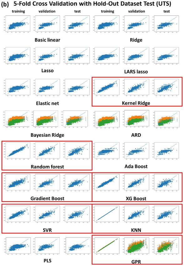
Figure 2 shows the plots of the predicted vs. experimental YS and UTS, wherein the training, validation and
test datasets for the fivefold cross validation led to a relatively good fit only for the seven nonlinear regression
algorithms KRR, RF, Gradient boost, XG boost, SVR, KNN and GPR (marked as red boxes), but the basic and
regularization-involved linear regression and PLS algorithms were far worse by comparison with the seven non-
linear regression algorithms. The same trend was detected in the sixfold cross validation results, which is available
in the “Supplementary Information” (Fig. S1). ANN (or DNN) results were omitted from Table 1 and from Figs. 1
and 2, because the regression results were well described in the previous r eport19. The regression fitting quality
for the DNN in the previous report was as good as those for the seven nonlinear regression algorithms. Conse-
quently, the linear regression algorithms gave rise to the poorest regression results. The regularization-involved
linear regression algorithms such as Ridge, LASSO, Elastic net, BRR, and ARD were never successful, and the
absolute MSE and R2 levels were unacceptable and equivalent to the basic linear regression, as shown in Table 1
and in Fig. 2. Of the regularization-involved linear regression algorithms, only the KRR was acceptable. Although
the main function of KRR is based on regularized linear regression, it could be regarded as a typical non-linear
regression algorithm due to the use of kernels (we adopted a matern kernel through the hyper-parameter optimi-
zation procedures). The regularized linear regression algorithms work best in the case of linear problems with a
small dataset (data paucity cases, normally). By contrast, our TMCP steel dataset had a non-linear nature with a
dataset size that could be considered moderate, which is compatible with the size of the problem. This led to us to
conclude that the TMCP steel dataset size was sufficiently large and no regularization was necessary. In addition,
the PLS conferred an unacceptable regression quality, which could be rationalized by invoking the fact that the
PLS algorithm is another type of linear regression, which would naturally give a poor regression result. The PLS
algorithm is known to work best for a linear problem particularly when the number of data points is fewer than
the number of d escriptors34. That was not the case, however, for the TMCP steel dataset.
The ensemble algorithms returned promising regression results, thanks to their non-linear regression capa-
bility. It is interesting, however, that Ada boost had a poor regression result. The poor fitting quality for Ada
Scientific Reports | (2021) 11:11012 | https://doi.org/10.1038/s41598-021-90237-z 3
Vol.:(0123456789)
www.nature.com/scientificreports/
Figure 1. The training, validation and hold-out dataset test results for the seven non-linear ML algorithms in
terms of (a) MSE and (b) R2 for 6- and 5-fold cross validation with a holdout dataset test, (c) the over-fitting
alidation_R2/Training_R2 and Test_R2/Training_R2.
index defined as V
boost was due to a choice of basic estimators that differed from that of the other ensemble algorithms. As
already discussed above, decision trees with some depth levels were adopted as a basic estimator for the other
three ensemble algorithms such as RF, Gradient boost, and XG boost. On the other hand, Ada boost employed
a so-called stump that consists of a one-level decision tree, i.e., uses only a single attribute for splitting. In this
regard, the model complexity for Ada boost has been significantly reduced so that it resembles a simple linear
regression. Consequently, the higher complexities of the RF, Gradient boost, and XG boost algorithms were
appropriate for the present non-linear problem.
As shown in Fig. 2, the BRR, ARD, and GPR regression based on the Bayesian approach produced conspicu-
ous and distinctive regression results. Bayesian approach-involved algorithms give a range of confidence (error
range) around the predicted mean rather than a deterministic prediction. The amber and green dots for the BRR,
ARD, and GPR results designate the upper and lower confidence boundaries, as shown in Fig. 5. These Bayesian
approaches are more favorable than the customary regression strategies due to the fact that uncertainty in the
prediction can also be formulated. It is noted, however, that this sort of merit for the Bayesian approach did not
take effect for the BRR and ARD algorithms because they were poorly fitted. It should be noted that BRR and
ARD were still based on a linear regression. Only GPR algorithms capable of accommodating the non-linearity
problem exhibited acceptable regression results, along with reasonable upper and lower confidence boundaries.
In addition to the fitting quality (bias issue) parameterized via MSE and R 2, the over-fitting (variance) issue
should be carefully taken into account when judging the regression fit. The ratio between the training and valida-
tion of R 2 could be indicative of the level of over-fitting, which is referred to as the ‘over-fitting index’. Figure 1c
shows the over-fitting index in a range of from 0.65 to 0.92, which is defined as V alidation_R2/Training_R2. A
higher over-fitting index indicates a better fit, i.e., 1 is reached in an ideal case. Figure 1c also shows the over-
fitting index, defined as the Test_R2/Training_R2, which is similar to the Validation_R2/Training_R2. However, the
over-fitting index would not matter for linear regression-based algorithms with a poor fitting quality, because the
overfitting issue matters only under the premise that the regression results for a training dataset are acceptable—
the overfitting index make sense only when the regression is not poorly fitted. Thus, the over-fitting index stood
out only for the seven non-linear regression algorithms. Although all the linear regressions gave rise to quite an
acceptable over-fitting index, it is futile to mention it since they were extremely biased (poorly fitted). Figure 2
shows such a seriously biased result for all the linear regressions. The seven non-linear regression algorithms
raised no serious over-fitting issues, according to the evaluated over-fitting index values that are greater than 0.6.
We focused on real-world data of a dirty nature in the present investigation. The connotations of the term
’dirty’ is a data distribution-related problem. The collected data are not identically and independently distrib-
uted (IID) random data, and the distribution for some input features (descriptors and attributes) is discrete
and biased. ML works if the output loss (the squared residual between real and model-predicted outputs) can
Scientific Reports | (2021) 11:11012 | https://doi.org/10.1038/s41598-021-90237-z 4
Vol:.(1234567890)
www.nature.com/scientificreports/

                                  Figure 2.  Plots of predicted vs. experimental (a) YS and (b) UTS for training, validation and hold-out test
                                  datasets for 5-fold cross validation.

Scientific Reports |   (2021) 11:11012 |               https://doi.org/10.1038/s41598-021-90237-z                                                 5

                                                                                                                                             Vol.:(0123456789)
www.nature.com/scientificreports/
Figure 2. (continued)
be approximated to a Gaussian distribution. The input-feature distribution does not necessarily have to be an
IID-Gaussian distribution. However, such a highly biased non-IID data distribution would not be beneficial to
ML regression. A conventional pair distribution representation of data distribution confirmed the highly biased,
non-IID data nature in our previous report19, which also is reconfirmed by the HRS representation of the data
distribution in Fig. 3b. The HRS plot is much easier to read than the typical pair-wise 2-D distribution plot.
NSGA‑II execution for optimization of KRR, RF, Gradient boost, XG boost, SVR, KNN, and
GPR regression results. The NSGA-II was employed for an inverse design (prediction) using fully trained
Scientific Reports | (2021) 11:11012 | https://doi.org/10.1038/s41598-021-90237-z 6
Vol:.(1234567890)
www.nature.com/scientificreports/
Figure 3. (a) HRS operation principle; four 10-level-descretized input features (x 1–x4) with four different
periodicities, 2L for x1, 1/5L for x2, 1/50L for x3, and 1/500L for x4 (L is the full width of the HSR plot). z1 is a
new HRS-merged input feature representing x1–x4. (b) the TMCP steel dataset distribution plotted on the HRS
representation space. Six pair-wise 2-D scatter plots consisting of z 1–z4, visualize the data distribution in much
simpler manner. (c) alternative xi-zj feature mapping and (d) the corresponding15 pair-wise 2-D HRS scatter
plots consisting of z1–z6.
Scientific Reports | (2021) 11:11012 | https://doi.org/10.1038/s41598-021-90237-z 7
Vol.:(0123456789)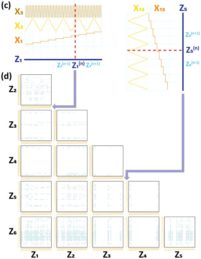
www.nature.com/scientificreports/
Figure 3. (continued)
KRR, RF, Gradient boost, XG boost, SVR, KNN, and GPR regression models. The objective functions (output
features: YS and UTS) were maximized by adjusting a decision variable (input feature, descriptor, or attribute:
x1–x16) based on a principle of natural selection that involves both the principles for excellency preservation
and diversity pursuit. To achieve multi-objective optimization, the NSGA was developed by employing a Pareto
optimality theory, and was reinforced by a large-scale elitism s trategy39. The elitist-reinforced NSGA, the so-
called NSGA-II38, is a very robust multi-objective optimization algorithm for materials discovery50–53, but its
performance is restricted to double-objective p roblems40,41. The NSGA-III was recently introduced to tackle
multi-objective optimization issues40,41. In this context, we adopted the NSGA-II since we dealt with only two
objective functions, YS and UTS, in the present investigation. A more detailed introduction for NSGA-II is aptly
described in our previous reports50–53.
Scientific Reports | (2021) 11:11012 | https://doi.org/10.1038/s41598-021-90237-z 8
Vol:.(1234567890)
www.nature.com/scientificreports/
GAs have previously been used in association with A NNs5,19,35–37,42–44. In those cases, however, single-objective
problems were the only concern. Neither NSGA-II nor NSGA-III has ever been used for an inverse prediction
based on any type of ML regression model. The objective functions of our optimization problem were YS and
UTS, which are the output features for all of the ML models, and the decision variables were the 16 input fea-
tures. Both objective functions should be simultaneously maximized via NSGA-II iteration. We repeated the
NSGA-II execution 200 times for each ML algorithm. Each NSGA-II execution produced 200 generations with
a population size of 50 per each generation. Every NSGA-II execution provided a very narrow Pareto frontier
in the last (200th) generation, so that we randomly collected one representative solution from the first Pareto
frontier in the last generation for each NSGA-II execution. In other words, each NSGA-II execution yielded 200
generations and the last (200th) generation showed an inordinately concentrated objective function space so
that the Pareto sorting of this final solution ended up with only a few concentrated Pareto groups. Consequently,
we finally collected a solution from the first Pareto frontier of the 200th generation for each NSGA-II execution
and eventually a total of 200 solutions for each ML algorithm.
Those who are not completely familiar with the NSGA-II algorithm would misunderstand that NSGA-II only
works best for what is known as a compromise (trade-off) problem. As can be clearly seen in Fig. 4, the YS-UTS
relationship is not trade-off, but roughly a linear relationship. The NSGA-II worked out, however. Because the
YS-UTS plot has a broad distribution (although the overall shape is roughly linear), the NSGA-II searched a
Pareto frontier in such a broad YS-UTS distribution. More importantly, the objective functions that are not in
the trade-off relationship are still applicable for NSGA-II algorithms. The point is that the NSGA-II algorithm
was designed for trade-off problems, but it works well for non-trade-off cases as well.
Rather than pursuing diversity, the convergence seemed to take place preferably while 200 generations were
produced for a single NSGA-II execution. To artificially secure a certain extent of diversity we executed the
NSGA-II execution independently 200 times for each ML algorithm, and collected the final solution by nomi-
nating one solution from each NSGA-II execution. Figure 4 shows those solutions in the objective function
space for each of the ML algorithms. Therefore, the final inverse prediction results involving 200 solutions for
each of the ML algorithms (200 TMCP alloy candidates) are graphically represented in Fig. 4. The solutions
from KRR, SVR, and GPR are concentrated in a small region, but those from KNN, RF, Gradient boost, and
XG boost are distributed across a relatively large area. Except for the solution of the inverse prediction result for
Gradient boost, all the others overlapped considerably with the experimental data in the high YS/UTS region.
The Gradient Boost solution is distinctively located in a large area beyond the experimental data. According to
the ML fundamentals, this sort of outstanding result for the Gradient boost would not be welcome but rather
apt to be discarded since it could be an awkward outcome originating from severe overfitting. It is pointless to
expect any type of ML algorithm to predict some excessively promising output by comparison with the train-
ing data. In terms of both diversity and excellency, the XG Boost solution would be the most promising of the
seven ML algorithms. The KNN, KRR, SVR, RF, and GPR solutions seem a bit less promising since they exhibit
both narrower distributions (low diversity) and lower values for YS/UTS (low excellency) by comparison with
the XG boost solution. However, the lesson we must learn from the above-described inverse prediction result
is that there is no point in finding an algorithm that outperforms the others. Instead of using a single superior
model, it makes more sense to average the outcome of all the seven ML algorithms when predicting YS/UTS.
As Fig. 4 shows, all solutions are concentrated in a high YS/UTS area and mostly overlap one another. It
should be noted that almost all multi-objective optimization studies deal with the diversity in the objective
function (fitness) space. Diversity in the decision variable space has never been studied extensively, although
there have been attempts to deal with this issue54. It is also important to examine the diversity issue in the deci-
sion variable (input feature) space and more importantly, the overlap between inverse-predicted solutions from
different ML algorithms in the decision variable space should be systematically examined. For this sake, it is
worthwhile to visualize the solution (the inverse prediction result) in the decision variable (input-feature) space.
The solution points in the input-feature space were visualized using HRS, as shown in Fig. 5. Figure 6 shows the
same data represented using a different HRS setting with better resolution, as discussed in the Computational
details section. The YS/UTS value can also be plotted in terms of hue in the HRS space, which is available in the
“Supplementary Information” (Fig. S2).
The solution distribution in such a high dimensional input-feature (decision variable) space differed from one
ML algorithm to another. This means that the terrain of the predicted objective function (output feature) differed
for each of the fully trained ML models. The KRR, SVR, and GPR returned a narrow solution distribution not
only in the objective function space Fig. 4 but also in the decision variable space (Figs. 5 and 6), meaning that
the objective function terrain for the fully trained KRR, SVR, and GPR might be similar to a uniquely convex
topography, while the KNN, RF, Gradient boost, and XG boost resulted in a highly diverse and wider solution
distribution, implying that the objective function terrain for the fully trained KNN, RF, Gradient boost, and XG
boost should be bumpier in the 16-dimensional decision variable space. In scrutinizing the solutions, it appears
that a certain portion of KRR and SVR solutions overlapped in the HRS space. Also, the GPR solution does not
seem to heavily deviate from those for both KRR and SVR. The solution distribution for the KNN, RF, Gradi-
ent boost, and XG boost algorithms were so widely scattered that the solutions considerably overlapped one
another and also overlapped the solutions from KRR, SVR, and GPR. All the solutions for every ML algorithm
are co-plotted with different colors in Fig. 5h, showing the overlap in some areas (although it looks disordered).
It is evident that every ML algorithm gave rise to different inverse predictions despite a certain degree of
overlap. To maximize the objective function (YS/UTS) values, NSGA-II herded alloy candidates in a high YS/
UTS direction, which differed from one ML algorithm to another. A clear finding is that the NSGA-II execution
worked well for all seven of the ML algorithms, but the finally optimized solutions were highly diverse depend-
ing on the selected ML algorithm, and there was no common global optimum, meaning that the solutions were
not uniquely converged on a narrow area but scattered across a large input feature space. The exceptions were
Scientific Reports | (2021) 11:11012 | https://doi.org/10.1038/s41598-021-90237-z 9
Vol.:(0123456789)www.nature.com/scientificreports/
Figure 4. The inverse-predicted (NSGA-II-maximized) YS and UTS for (a) KRR, (b) SVR, (c) GPR, (d) RF,
(e) Gradient Boost, (f) XG Boost, and (g) KNN regression models, obtained from the NSGA-II-driven inverse
prediction for the seven non-linear ML algorithms along with the entire dataset, marked in different colors. (h)
the merged solutions from all the seven ML algorithms. The entire dataset was also plotted as a background.
the KRR and SVR solutions that clearly overlapped within a narrow region. A more serious issue, however, is
the fact that some of the solutions from all the algorithms were located out of the training data distribution. To
confirm this, we plotted all the data for the 5473 TMCP alloys as background for all of the HRS plots in order
accomplish systematic comparisons, as shown in Fig. 5. Many of the solutions were located either inside or nearby
the training data area, but some were located far away from the training data distribution.
Those with a dearth of knowledge concerning ML might unconditionally welcome higher YS/UTS predic-
tions without checking on the decision variable space. If the training dataset had a continuously dispersed data
distribution, the prediction results would have been more reasonable. On the contrary, if a dataset exhibits a
highly biased, skewed, discrete distribution similar to our TMCP steel dataset, then an in-depth examination
of the solution space (= decision variable space = input feature space) should definitely be accounted for along
with the conventional examination of objective function space. It is necessary to investigate an extremely high
dimensional solution space. Although we introduced the HRS graphical representation in order to visualize the
16-D solution space, the HRS approach remains far from complete. We still need to examine the six 2-D HRS
plots (or 15 2-D HRS plots) at the same time to completely understand the data status. It should, however, be
noted that with the introduction of HRS, the 120 2-D plots for the conventional pair-wise data representation
have been significantly reduced to just six (or 15) plots.
It is not surprising that the seven well-established ML algorithms ended up with quite different inverse-
predicted solutions, albeit with a certain degree of overlap. The ML and metaheuristics never gave a definite
common global optimal solution, but instead every ML algorithm gave rise to their own unique solution. On this
ground, it would be extremely risky to select an ML algorithm only by relying on the goodness of fit, since we
confirmed that the selected seven ML algorithms exhibited quite a satisfactory goodness of fit with very different
solutions. Although all the ML algorithms exhibited similar inverse-predicted YS/UTS values, they are widely
dispersed in the high dimensional solution space. The data-driven approach is not like a traditional rule-based
analysis that leads to consistent, definite outcomes under all circumstances. Due to the heuristic, ad-hoc nature of
data-driven approaches, each of the seven ML algorithms led to quite a scattered inverse-predicted result differing
from one another. Therefore, the adoption of a particular ML algorithm selected on the basis of the goodness of
fit for a certain problem would be risky. Instead, a group of ML algorithms similar to our so-called “integrated
ML platform” should be adopted for a single problem with a single dataset. By doing so, various solutions could
be attained. Thereafter, final solutions could be recommended by analyzing a variety of the solutions that result
from various ML algorithms.
Although we provided all the inverse-predicted solutions from the seven ML algorithms and also graphically
recommended some overlapped solutions, we did not extensively examine them in terms of the materials side
in contrast to our previous r eport19 wherein the materials side of selected candidates were examined in detail.
Several alloys that were inverse-predicted by ANN/NSGA-II algorithms in our previous r eport19 overlap with the
solution in the present investigation. The previous solution was validated by field experts and also backed up by
well-established theoretical calculation (e.g., thermos-Calc.)55, through which the Ae1 and Ae3 temperatures were
calculated and the precipitation reactions of (Ti,Nb)C and VC were evaluated. The calculated thermodynamic
conditions from the previous solution are quite reasonable in terms of conventional hot rolling and subsequent
heat-treatment processes. Accordingly, the solution in the present investigation could be equally interpreted by
Scientific Reports | (2021) 11:11012 | https://doi.org/10.1038/s41598-021-90237-z 10
Vol:.(1234567890)www.nature.com/scientificreports/
Figure 5. The HRS representation of inverse-predicted solutions for (a) KRR, (b) SVR, (c) GPR, (d) RF,
(e) Gradient Boost, (f) XG Boost, and (g) KNN regression models, plotted on the HRS represented input
feature space, consisting of six pair-wise 2-D scatter plots consisting of z 1–z4, which are considered as an HRS
representation unit. The entire dataset was also plotted as a background and the solutions from each ML
algorithm are highlighted in dark red color. (h) The solutions from all the seven ML algorithms are merged in
a single HRS representation unit. Each axis for the six pair-wise 2-D plots designate z 1–z4, and the formulation
principle for z 1–z4 was presented in Fig. 3a.
Scientific Reports | (2021) 11:11012 | https://doi.org/10.1038/s41598-021-90237-z 11
Vol.:(0123456789)www.nature.com/scientificreports/
Figure 6. Alternative HRS representation; 15 2-D HRS plots involving six z j features (four zj features ( z1–z4),
each of which was mapped from three xi features and two zj features ( z5 and z6) from two xi features per each),
considered as an HRS representation unit. Inverse-predicted solutions for (a) KRR, (b) SVR, (c) GPR, (d) RF,
(e) Gradient Boost, (f) XG Boost, and (g) KNN regression models. The entire dataset was also plotted as a
background and the solutions from each ML algorithm are highlighted in dark red color. (h) The solutions from
all the seven ML algorithms are merged in a single HRS representation unit.
Scientific Reports | (2021) 11:11012 | https://doi.org/10.1038/s41598-021-90237-z 12
Vol:.(1234567890)www.nature.com/scientificreports/
refereeing to the previous result. An in-depth study of the performance and microstructures of the predicted
materials will be dealt with separately in the near future. Of course, most of the alloy candidates suggested by the
integrated ML platform (listed in Table S1) were within a reasonable range by referring to the common sense of
field experts. The amount of C, Mn, Nb, and Si was well controlled by the NSGA-II optimization process and the
increased amount of these key components in the solution seemed contributive to improving the strength and
positive for the TMCP application. The massive solution data presented in Table S1 were succinctly rearranged
as 1-D distribution plots for every input feature as shown in Fig. S3, wherein one can clearly detect a narrowed
solution range in comparison to the entire dataset distribution.
The scope of the present investigation was limited to a methodology introduction in order to accomplish
an efficient data-driven metal alloy design, and also to warn materials scientists regarding the ad-hoc, heuristic
nature of ML approaches. A key lesson that we have learned from the present study is that we must not blind-
trust the ML-based, inverse-predicted result unless the solution distribution in the input feature space is precisely
examined by employing at least more than several ML algorithms simultaneously.
Computational details
Data acquisition and descriptor extraction. The dataset acquired from Hyundai Steel Co. included
5473 alloy entries with 14 alloy components, two processing variables, and the two materials properties of yield
strength (YS) and ultimate tensile strength (UTS). X 1–14 are the elemental compositions for C, Si, Mn, P, S, Cu,
Sn, Ni, Cr, Mo, V, Nb, Ti, and Ca. X 15 and X 16 represent heating time and temperature, respectively. All the
other processing conditions were fixed. Since the dataset was gleaned from real-world industry, better-organized
features representing microstructural and physical attributes were not available, although a recent trend is to
introduce intermediate descriptors to enhance predictability2. Consequently, the problem was simply set up with
16 input features and 2 output features. All the input/output features were min–max-normalized such that each
feature ranged from 0 to 1, The distribution of each feature was well-described in the previous r eport19.
It is obvious that some of the input features could not approximate a continuous random variable, but these
were in a highly biased and discrete state, and some of the continuous variables were not in a unimodal normal
distribution, but were, instead, in the form of multi-modal distributions. The so-called ‘dirty nature’ of the dataset
was confirmed by both pair-wise data distribution plots and Pearson correlation analysis, which also revealed
no severely correlated feature pairs in our dataset. However, we did not employ systematic ways of mapping data
from various distributions to a normal distribution such as that seen in Box–Cox56, Yeo–Johnson57, and Quantile
transformations58, since the conventional ML approach places no strict restrictions on the input data distribution.
Note that the only restriction of the ML data is that the residual (difference between real and ML-predicted output
feature) should be in a normal distribution, which refers to the L2 loss minimization (= the maximum likelihood
estimation) that is a crucial prerequisite for successful ML. If this condition is met, the training dataset requires
no other restrictions. Nonetheless, the dirty nature of the dataset would not seem favorable for the ML-based
regression and the ensuing inverse prediction process.
The highly biased discrete data status was visually represented as 120 2-dimensional pair-distribution plots
along with a Pearson coefficient matrix in the previous report19. Such intricate data visualization complicates
the data status. Many high-dimensional data visualization techniques have been reported thus far. These include
the pair-wise scatter plot that we used in the previous report19, a pair-wise correlation matrix and h eatmap59, a
tree diagram (dendrogram)60, Chernoff f aces61, and many more62. In addition, more advanced strategies that are
based on both statistical science and machine learning are also available for high-dimension complicated data,
which is referred to as ‘big data’ in many domains. These types of data reduction and visualization strategies
include early-stage basic algorithms such as principal component analysis (PCA)63 and classical multidimensional
scaling (MDS)64, along with more advanced recent algorithms such as stochastic neighbor embedding (SNE and
t-SNE)65,66, and more recently developed algorithms such as uniform manifold approximation and projection
(UMAP)67, ChemTreeMap68, tree map (TMAP)69, and the Potential of Heat-diffusion for Affinity-based Transi-
tion Embedding (PHATE)70.
Although many high-dimensional data visualization strategies have been r eported59–70, none were adequate
for our 16-dimensional data visualization. A typical PCA-based data dimension reduction and the ensuing
2-D projected data visualization causes too much information loss in the course of the data reduction process.
We adopted an alternative multi-dimensional data visualization methodology referred to as the holographic
research strategy (HRS), which was developed by Margitfalvi et al.45–48. The HRS can effectively visualize a high-
dimensional dataset and minimize the loss of data information. Although the above-described high-dimensional
data visualization strategies have been used for many problems in various domains, the HRS has not been widely
utilized. It should be noted, however, that the HRS has been successfully used for the discovery (optimization)
of multi-compositional inorganic c atalysts45–48. Our understanding is that HRS deserves to be spotlighted since
its potential for multi-dimensional data visualization is promising in cases where the dimensions of the data are
not too high (< 20).
We combined four input features as a single feature in the manner described in Fig. 3a: x1–x4 as z 1, x5–x8 as
z2, x9–x12 as z3, and x13–x16 as z4. There are a large number of different combinations, any of which are accept-
able. First, all the x i features were discretized such that the min–max-normalized x i feature (in the range 0–1)
was classified into 10 levels. Thereafter, every x i feature was rearranged as a periodical with the same amplitude
(= 10 levels) but with a different periodicity. Thereafter, four xi features with different periodicities were stacked
one-on-another in turn as shown in Fig. 3a, and the vertical red dashed line bisecting all four xi periodicals at
different levels for each x i feature ultimately constitute a certain single z j value at the bottom. This means that the
zj value exactly represents those four x i feature values that come across the vertical red line. In this way, the four
dimensional input features (e.g. x 1–x4) were mapped to one dimensional feature ( z1) with no loss of information.
Scientific Reports | (2021) 11:11012 | https://doi.org/10.1038/s41598-021-90237-z 13
Vol.:(0123456789)www.nature.com/scientificreports/
Of course, we ignored a small amount of information loss caused by the x i feature discretization process. Conse-
quently, the 16-dimensional input features (xi, i = 1–16) were efficiently reduced to 4-dimensional input features
(zj, j = 1–4), and thereafter any of the pairs out of the four z j features could be drawn on a typical 2-dimensional
(2-D) pair-wise plot, and eventually six 2-D plots could represent the original 16-dimensional data distribution.
Figure 3b shows six 2-D scatter plots (so-called 2-D HRS plots) elucidating the total data distribution that
the four z js (z1–z4) constitute. By comparison with a conventional pair-wise scatter plot using 16 x i features that
produce 120 2-D pair-wise plots, only six pair-wise scatter plots using four z j features should be much more suc-
cinct and easier to understand. Finally, the TMCP steel dataset plotted on the HRS representation space shown
in Fig. 3b also exhibits a very scattered, biased, and non-IID data status, as already proven in the conventional
120 pair-wise scatter plots in our previous report48. The YS and UTS were also plotted on the HRS representation
space in terms of the hue, as shown in Fig. S5, which is available in the “Supplementary Information”. Figure S5
shows that no conversed area exhibiting high YS/UTS values exists on the HRS representation space, which
implies that simple linear regression ML models would not suffice in this complicated 16-dimensional input
feature space.
The xi feature with the highest frequency (the smallest periodicity) would lose its resolution on the 2-D HRS
diagram and make the HRS representation impractical. Note that the fourth xi feature had a periodicity of 1/500L.
Unless the 2-D HRS plot were zoomed in, the fourth x i feature would have no effect. If a zj feature is mapped
from three (or two) xi features, then adequate resolution can be ensured on the 2-D HRS plot. In such a case, we
have six zj features that result in fifteen 2-D HRS plots. Figure 3c elucidates the xi-to-zj feature mapping process
schematically: x1–x3 as z1, x4–x6 as z2, x7–x9 as z3, x10–x12 as z4, x13–x14 as z5, and x15–x16 as z6. The fifteen 2-D HRS
plots (Fig. 3d) are much easier to read than the original 120 plots, although the fifteen plots still seem inordinate
when compared to the six 2-D HRS plots with four zj features (Fig. 3b). Figure 6 shows fifteen 2-D HRS plots
involving six zj features to visualize the inverse-predicted solutions for the seven ML algorithms. There would
be no information loss caused by a high frequency x i feature when a z j feature was mapped from two or three xi
features. Those who are uncomfortable with the six 2-D HRS plots can refer to Fig. 6. However, the six 2-D HRS
plots along with four z j features, as shown in Fig. 3b, still have reasonable resolution in comprehending the data
distribution. In addition, it is also possible to create a 3-D HRS plot as shown in Fig. S5. Despite the advantage
that only a single 3-D HRS plot is sufficient to visualize the 16-dimensional input feature space, the 5-level dis-
cretization of xi features was inevitable since each zj feature is mapped from six or five xi features. The sparser xi
feature discretization and the higher frequency would never lead to proper resolution in this 3-D HRS plot and
a considerable information loss would be unavoidable.
ML model selection. In this study we reviewed three categories of ML algorithms involving 16 versions.
The first category includes the so-called regularized linear regression algorithms: Ridge regression, least absolute
shrinkage and selection operator (Lasso) regression, least-angle regression (LARS), elastic net regression (ENR),
kernel ridge regression (KRR), Bayesian ridge regression (BRR), and Bayesian automatic relevance determina-
tion (ARD). Basic linear regression was also incorporated in this first group as a baseline method. L2 (Ridge)
and L1 (Lasso) regularizations are the most generally adopted form of regularization. L2 and L1 regularizations
incorporate the L2 and L1 norms of weights as a penalty in the loss function. Other supplementary regulariza-
tion algorithms such as LARS, KRR, BRR, and ARD are also employed. The LARS algorithm is a special version
of the Lasso problem. In order to account for non-linearity, the KRR algorithm incorporates kernels such as
polynomial, radial basis function (RBF), sigmoid, and matern. The BRR and ARD algorithms incorporate the
Bayesian approach. The Bayesian approach is used for BRR and ARD regressions, which are used to make a final
prediction that is distributive rather than deterministic. The prediction is not deterministic because it is made
with a certain mean and variance originating from the fact that the fitted parameters are distributed rather than
deterministic.
The second category includes ensemble algorithms. The ensemble algorithm model consists of a collection of
individual small models (base estimators). The predictability of an individual model is limited since it is likely to
give rise to over-fitting, but combining many such weak models in an ensemble leads to a much improved level of
predictability. The most common individual weak model is a decision tree with different depths determined by
the chosen algorithm. For example, Ada boost uses stumps that are trees with only a single-level depth and the
other ensemble algorithms use trees with deeper depth levels. We employed several tree ensemble algorithms such
as random forest (RF), adaptive (Ada) boost, Gradient boost, and extreme Gradient (XG) boost. The ensemble
algorithm generally has two representative model implementations, i.e., bagging and boosting. The bagging is
for use with RF and each base model is treated independently, while the boosting for use with Ada, Gradient,
and XG boost algorithms sequentially place greater weight on the data of each model (on the feature), which
could connect the wrong predictions and result in high rates of error.
We also incorporated some non-linear regression ML algorithms such as support vector machine regression
(SVR), k-nearest neighbors (KNN), and Gaussian process regression (GPR). An additional linear regression algo-
rithm, partial least square (PLS), was also introduced. Prior to the advent of deep learning, SVR outperformed
conventional ANNs in sorting out many problems. The use of kernels such as polynomial, radial basis function
(RBF), sigmoid, and matern kernels is essential for SVR and an RBF kernel was selected from the hyper-param-
eter optimization process for the present SVR. KNN, which is known as the simplest ML algorithm, is strongly
dependent on an ad hoc determination of appropriate k values. Therefore, we obtained the best k value from the
hyper-parameter selection procedures. GPR, so-called kriging, has recently attracted a great deal of attention
as it often has been used as a surrogate function for Bayesian optimization71. As with BRR and ARD regression
algorithms, the GPR prediction was also made with a certain mean and covariance. In particular, we noted that
KNN and GPR are parameter-free (or model-free) ML algorithms that differ from most other ML algorithms
Scientific Reports | (2021) 11:11012 | https://doi.org/10.1038/s41598-021-90237-z 14
Vol:.(1234567890)www.nature.com/scientificreports/
Figure 7. The overall graphical description for the integrated ML platform. Three groups of ML algorithms, the
NSGA-II-driven inverse prediction, and the high-dimensional data visualization method are given.
that aim to search for optimal parameters constituting a ML model. PLS is a traditional linear regression method
that is even applicable to problems with fewer data points than the number of input features, which is a situation
far from ours. Our problem was ameliorated by considering the dataset size (5473 data points) relative to the
number of input features (16). More interestingly, we omitted ANN here since it had already been employed for
the same regression in our previous report19. Several ML algorithms were used for the ensuing inverse predic-
tion based on the NSGA-II, although only the ANN(= DNN) was used for the inverse prediction in the previous
report19. Figure 7 features a succinct schematic that describes the entire ML platform and the ensuing inverse
prediction process as well as the high-dimensional data visualization. All the above-described regression algo-
odule72 with well-established default hyper-parameters, some of which
rithms are available in the Scikit-learn m
were incorporated here. We performed a hyper-parameter optimization process, however, to determine some of
the key hyper-parameters. The hyper-parameter screening process will be discussed in the following subsection.
Training, validation, and test dataset splitting. Meticulous care should be taken when splitting the
data into training, validation, and test datasets. Only a simple split into training and test datasets was not viable.
We adopted two training schemes. First, we adopted a sixfold cross-validation73–75 scheme without preparing
a holdout test dataset, and the results of validation were used for the hyper-parameter screening. Second, we
set aside a holdout test dataset that included 913 alloys, and a 5-fold cross-validation was implemented for the
remainder of the data, which included 4560 alloys. We then tested the fully trained model using the holdout
test dataset. The optimal hyper-parameters obtained from the preceding 6-fold cross-validation process were
employed for the ensuing 5-fold cross-validation and test processes.
Hyper-parameter optimization is one of most important ML issues that has been developed in recent years,
and the most efficient way of tackling the issue is the use of Bayesian optimization71. Differing from typical deep-
learning cases, however, the present problems of a moderate size did not require such an additional high-cost
Scientific Reports | (2021) 11:11012 | https://doi.org/10.1038/s41598-021-90237-z 15
Vol.:(0123456789)www.nature.com/scientificreports/
optimization strategy. Instead, we designed an enumerable hyper-parameter search space (mesh) for each algo-
rithm. Each mesh involved a tractable number of hyper-parameter sets that amounted to approximately 100
for testing (the maximum number of hyper-parameter sets was at best 144 for a Gradient boost algorithm).
We screened all the hyper-parameter sets by monitoring the validation MSE and R2 results evaluated from the
6-fold cross-validation, and eventually pinpointed an optimal hyper-parameter set for each algorithm. All the
hyper-parameter sets with their validation MSE and R 2 values are given in Table S2, wherein the finally selected
hyper-parameter set for each algorithm is highlighted.
Conclusions
An integrated ML platform involving 16 algorithms was developed to achieve YS/UTS predictions from compo-
sitional and processing descriptors. The 5473 TMCP steel alloys gleaned from the real-world industry were used
to establish training, validation, and test datasets for use with an integrated ML model platform.
Nonlinear ML algorithms outperformed the basic linear regression algorithm as well as its regularized ver-
sions. Well-known non-linear regression algorithms such as KRR (with a matern kernel), RF, Gradient boost,
XG boost, KNN, SVR, and GPR worked properly but all the others proved to be unacceptable. These seven fully
trained non-linear ML algorithms were used to make NSGA-II-driven inverse predictions, and some desirable
solutions were obtained.
In addition, the solutions were graphically visualized not only in the conventional low-dimensional objective
function space but also in the 16-dimensional decision variable space using the HRS technique, so that the data
status could be comprehended in a systematic manner. By visualizing the solution in the input feature space, a
real-sense ML prediction was achieved. The ML algorithms never gave a common optimal solution, but every
ML algorithm predicted a very diverse solution in the input feature space. We suggest that the adoption of either
a single or a few ML algorithms for alloy design is very risky and it also is extremely risky to select an ML algo-
rithm only by relying on the goodness of fit.
The amount of C, Mn, Nb, and Si was well controlled by the NSGA-II optimization process and the increased
amount of these key alloying elements in the solution contributed to improving the strength and played a positive
role for the TMCP application. The experimental validation should be the next step although most of the alloy
candidates suggested in the present investigation were within a reasonable range by referring to the common
sense of field experts.
Data availability
All data generated or analyzed during this study are included in this published article (and its “Supplementary
Information” files) and the datasets used for the integrated ML platform during the current study are available
from the corresponding author on reasonable request.
Code availability
The codes used for this study are available from the GitHub link at https://github.com/socoolblue/integrated_
ML_platform.
Received: 1 April 2021; Accepted: 10 May 2021
References
1. Guo, Z. & Sha, W. Modelling the correlation between processing parameters and properties of maraging steels using artificial
neural network. Comput. Mater. Sci. 29, 12–28 (2004).
2. Xiong, J., Shi, S.-Q. & Zhang, T.-Y. A machine-learning approach to predicting and understanding the properties of amorphous
metallic alloys. Mater. Des. 187, 108378 (2020).
3. Frank, E., Hall, M. A. & Witten, I. H. The WEKA Workbench. Online Appendix for “Data Mining: Practical Machine Learning Tools
and Techniques” 4th edn. (Morgan Kaufmann, 2016).
4. Möller, J. J. et al. Compositional optimization of hard-magnetic phases with machine-learning models. Acta Mater. 153, 53–61
(2018).
5. Shen, C. et al. Physical metallurgy-guided machine learning and artificial intelligent design of ultrahigh-strength stainless steel.
Acta Mater. 179, 201–214 (2019).
6. Zhang, H. et al. Dramatically enhanced combination of ultimate tensile strength and electric conductivity of alloys via machine
learning screening. Acta Mater. 200, 803–810 (2020).
7. Kaufmann, K. & Vecchio, K. S. Searching for high entropy alloys: A machine learning approach. Acta Mater. 198, 178–222 (2020).
8. Wang, Y. et al. Accelerated design of Fe-based soft magnetic materials using machine learning and stochastic optimization. Acta
Mater. 194, 144–155 (2020).
9. Khatavkar, N., Swetlana, S. & Singh, A. K. Accelerated prediction of Vickers hardness of Co- and Ni-based superalloys from
microstructure and composition using advanced image processing techniques and machine learning. Acta Mater. 196, 195–303
(2020).
10. Wen, C. et al. Machine learning assisted design of high entropy alloys with desired property. Acta Mater. 170, 109–117 (2019).
11. Feng, S., Zhou, H. & Dong, H. Using deep neural network with small dataset to predict material defects. Mater. Des. 162, 300–310
(2019).
12. Sun, Y. T., Bai, H. Y., Li, M. Z. & Wang, W. H. Machine learning approach for prediction and understanding of glass-forming ability.
J. Phys. Chem. Lett. 8, 3434–3439 (2017).
13. Ward, L. et al. A machine learning approach for engineering bulk metallic glass alloys. Acta Mater. 159, 102–111 (2018).
14. Ren, F. et al. Accelerated discovery of metallic glasses through iteration of machine learning and high-throughput experiments.
Sci. Adv. 4, eaaq1566 (2018).
15. Ward, L., Agrawal, A., Choudhary, A. & Wolverton, C. A general-purpose machine learning framework for predicting properties
of inorganic materials. NPJ Comput. Mater. 2, 16028 (2016).
16. Tripathi, M. K., Ganguly, S., Dey, P. & Chattopadhyay, P. P. Evolution of glass forming ability indicator by genetic programming.
Comput. Mater. Sci. 118, 56–65 (2016).
Scientific Reports | (2021) 11:11012 | https://doi.org/10.1038/s41598-021-90237-z 16
Vol:.(1234567890)You can also read