A renewed rise in global HCFC-141b emissions between 2017-2021
←
→
Page content transcription
If your browser does not render page correctly, please read the page content below

Research article
Atmos. Chem. Phys., 22, 9601–9616, 2022
https://doi.org/10.5194/acp-22-9601-2022
© Author(s) 2022. This work is distributed under
the Creative Commons Attribution 4.0 License.

                A renewed rise in global HCFC-141b emissions
                             between 2017–2021
          Luke M. Western1,2 , Alison L. Redington3 , Alistair J. Manning3 , Cathy M. Trudinger4 , Lei Hu1,5 ,
        Stephan Henne6 , Xuekun Fang7 , Lambert J. M. Kuijpers8 , Christina Theodoridi9 , David S. Godwin10 ,
             Jgor Arduini11 , Bronwyn Dunse4 , Andreas Engel12 , Paul J. Fraser4 , Christina M. Harth13 ,
               Paul B. Krummel4 , Michela Maione11 , Jens Mühle13 , Simon O’Doherty2 , Hyeri Park14 ,
              Sunyoung Park14 , Stefan Reimann6 , Peter K. Salameh13 , Daniel Say2 , Roland Schmidt13 ,
            Tanja Schuck12 , Carolina Siso1,5 , Kieran M. Stanley12 , Isaac Vimont1,5 , Martin K. Vollmer6 ,
           Dickon Young2 , Ronald G. Prinn15 , Ray F. Weiss13 , Stephen A. Montzka1 , and Matthew Rigby2
          1 Global   Monitoring Laboratory, National Oceanic and Atmospheric Administration, Boulder, CO, USA
                                        2 School of Chemistry, University of Bristol, Bristol, UK
                                                 3 Hadley Centre, Met Office, Exeter, UK
                   4 Climate Science Centre, CSIRO Oceans and Atmosphere, Aspendale, Victoria, Australia
        5 Cooperative Institute for Research in Environmental Sciences, University of Colorado, Boulder, CO, USA
             6 Empa, Swiss Federal Laboratories for Materials Science and Technology, Dübendorf, Switzerland
            7 College of Environmental and Resource Sciences, Zhejiang University, Hangzhou, Zhejiang, China
                                              8 A/gent b.v. Consultancy, Venlo, Netherlands
                                     9 Natural Resources Defense Council, Washington, DC, USA
                10 Stratospheric Protection Division, Environmental Protection Agency, Washington, DC, USA
                          11 Department of Pure and Applied Sciences, University of Urbino, Urbino, Italy
                      12 Institute for Atmospheric and Environmental Science, Goethe University Frankfurt,

                                                      Frankfurt am Main, Germany
                13 Scripps Institution of Oceanography, University of California San Diego, La Jolla, CA, USA
                 14 Department of Oceanography, Kyungpook National University, Daegu, Republic of Korea
            15 Center for Global Change Science, Massachusetts Institute of Technology, Cambridge, MA, USA

               Correspondence: Luke M. Western (luke.western@bristol.ac.uk, luke.western@noaa.gov)

                                   Received: 20 April 2022 – Discussion started: 27 April 2022
                             Revised: 21 June 2022 – Accepted: 7 July 2022 – Published: 28 July 2022

      Abstract. Global emissions of the ozone-depleting gas HCFC-141b (1,1-dichloro-1-fluoroethane, CH3 CCl2 F)
      derived from measurements of atmospheric mole fractions increased between 2017 and 2021 despite a fall in
      reported production and consumption of HCFC-141b for dispersive uses. HCFC-141b is a controlled substance
      under the Montreal Protocol, and its phase-out is currently underway, after a peak in reported consumption and
      production in developing (Article 5) countries in 2013. If reported production and consumption are correct,
      our study suggests that the 2017–2021 rise is due to an increase in emissions from the bank when appliances
      containing HCFC-141b reach the end of their life, or from production of HCFC-141b not reported for dispersive
      uses. Regional emissions have been estimated between 2017–2020 for all regions where measurements have
      sufficient sensitivity to emissions. This includes the regions of northwestern Europe, east Asia, the United States
      and Australia, where emissions decreased by a total of 2.3 ± 4.6 Gg yr−1 , compared to a mean global increase
      of 3.0 ± 1.2 Gg yr−1 over the same period. Collectively these regions only account for around 30 % of global
      emissions in 2020. We are not able to pinpoint the source regions or specific activities responsible for the recent
      global emission rise.

Published by Copernicus Publications on behalf of the European Geosciences Union.
9602                                                             L. M. Western et al.: A rise in global HCFC-141b emissions

1   Introduction

The global atmosphere has seen a decline in the burden of
most ozone-depleting substances since the implementation
of the Montreal Protocol on Substances that Deplete the
Ozone Layer (Engel and Rigby, 2019). Under the Protocol’s
framework, the global phase-out of production of chlorofluo-
rocarbons (CFCs) and halons for dispersive uses was report-
edly completed in 2010. The phase-out (with the exception of
very small amounts for the servicing of existing equipment)
of their controlled replacement gases, primarily hydrochlo-
rofluorocarbons (HCFCs), was completed in 2020 in devel-
oped (non-Article 5) countries, whilst developing (Article 5)
countries are in the process of a staged phase-out, to be com-    Figure 1. Global HCFC-141b production for dispersive uses (blue)
                                                                  and consumption (orange) reported to UNEP. Production of HCFC-
pleted by 2030.
                                                                  141b for use as a feedstock (green) is not included in the reported
   Despite a global ban on CFC production for dispersive
                                                                  total for dispersive production or compliance considerations with
uses, recent work found unexpected emissions of CFC-              respect to the Montreal Protocol.
11 (trichlorofluoromethane) between 2012 and 2017, likely
stemming from CFC-11 produced in violation of the Mon-
treal Protocol after 2010 (Montzka et al., 2018; Rigby et al.,
2019; Montzka et al., 2021; Park et al., 2021). These stud-       and destruction – exhibits two peaks (Fig. 1), one in 2002
ies provided evidence of renewed dispersive use of CFC-           and one in 2011. In addition to foam blowing, dispersive uses
11 in eastern China, which accounted for around 60 % of           for HCFC-141b are as an aerosol (1.4 Gg was consumed for
the concurrent increase in global emissions. Elevated emis-       aerosols in 2014 and 0.7 Gg in 2018) and a solvent (Multilat-
sions from eastern China of both CFC-12 and CCl4 , chemi-         eral Fund, 2019). The use of HCFC-141b for solvent clean-
cals involved in the production of CFC-11, from which they        ing has declined, from 4.7 in 2014 to 3.8 Gg yr−1 in 2018
can escape to the atmosphere, suggested that CFC-11 pro-          and is predicted to decline further (MCTOC, 2018; Multilat-
duction may have also occurred in this region. The most           eral Fund, 2019). HCFC-141b produced for use as a feed-
likely application of this newly produced CFC-11, which           stock is differentiated from dispersive production when re-
was not reported to the United Nations Environment Pro-           ported as its production quantity is not relevant for compli-
gramme’s (UNEP) Ozone Secretariat, was as a blowing agent         ance with the Montreal Protocol due to an earlier, but in-
for closed-cell foams (TEAP, 2019).                               correct, assumption of negligible emissions from feedstock
   The most widely used replacement gas for CFC-11 for            production and use (production for both dispersive uses and
foam blowing in developing countries was HCFC-141b (1,1-          feedstock is shown in Fig. 1). Production of HCFC-141b for
dichloro-1-fluoroethane, CH3 CCl2 F), which also has minor        feedstock was at a maximum of 18 Gg yr−1 in 2011, com-
applications as an aerosol, a solvent and feedstock and is        pared to 118 Gg yr−1 in 2011 for dispersive uses, and has re-
also an intermediate/by-product during the production of          mained at 12–13 Gg yr−1 between 2014–2020. However, the
other fluorochemicals. Under the phase-down schedule of           proportion of HCFC-141b produced as feedstock increased
the Montreal Protocol, HCFC-141b should no longer be pro-         from 12 % in 2014 to 23 % in 2020 due to the decline in
duced or consumed for dispersive uses in developed coun-          production for dispersive uses. HCFC-141b can be a feed-
tries, and production should be declining in developing coun-     stock, a by-product and a target product. Starting out from
tries since the HCFC phase-out began in 2013. HCFC-               methyl chloroform or vinylidene chloride (VDC), HCFC-
141b has a much shorter atmospheric lifetime than CFC-11          141b, HCFC-142b and HFC-143a are produced (Andersen
(around 9.4 compared to 52 years), and its potential to de-       et al., 2021). HCFC-142b can then be converted to vinyli-
plete stratospheric ozone is only around 0.07–0.10 times that     dene fluoride (VDF, HFO-1132a), a refrigerant and also the
of CFC-11 (Burkholder, 2019). Yet, HCFC-141b is still an          building block for the fluoropolymer polyvinylidene fluoride
ozone-depleting substance, with the potential to delay strato-    (PVDF). Any unwanted HCFC-141b can also be fed into
spheric ozone recovery, and, along with other HCFCs, it is        this production chain (TEAP, 2021; Andersen et al., 2021).
also a potent greenhouse gas, with a global warming poten-        While the size and exact fate of these production routes are
tial 800 times that of carbon dioxide over a 100-year time        not publicly known, it is possible that the market for PVDF
horizon (Burkholder, 2019).                                       is growing due to its use in Li-ion batteries and other high-
   Reported global HCFC-141b consumption – defined as             tech applications. Previous estimates of global HCFC-141b
production for dispersive uses plus imports minus exports         emissions, last reported up to 2016, based on atmospheric

Atmos. Chem. Phys., 22, 9601–9616, 2022                                             https://doi.org/10.5194/acp-22-9601-2022
L. M. Western et al.: A rise in global HCFC-141b emissions                                                                    9603

observations have generally been consistent with inventory
estimates, based on consumption reported to UNEP (neglect-
ing feedstock) and assumptions about rates of release to the
atmosphere (Montzka et al., 2015; Simmonds et al., 2017;
Engel and Rigby, 2019).
   Regional top-down (based on atmospheric measurements)
and bottom-up (based on assumptions about the size and rate
of release from various emissive processes and reported or
market-based estimates) HCFC-141b emission estimates are
sparse and exist only for northeast Asia, India, western Eu-
rope and the United States. Top-down emissions estimates
for China through 2017 by Fang et al. (2019b) show emis-          Figure 2. Locations of the AGAGE (pink circles) and NOAA
sions declining from 24 ± 5 to 15 ± 2 Gg yr−1 between 2011        (green circles) measurement stations used in this work to estimate
and 2017. A decline in Chinese emissions in recent years is       global and regional HCFC-141b emissions.
supported using a different set of atmospheric data by the es-
timates of Yi et al. (2021), albeit with smaller overall emis-
                                                                  2     Methods
sions, showing Chinese emissions peaking at 16 Gg yr−1 in
2014 and dropping to 11 Gg yr−1 by 2019 (uncertainties were
                                                                  2.1    Measurements
not given). Conversely, bottom-up estimates for China pro-
jected a peak in emissions in 2018 (26 Gg yr−1 ) (Wan et al.,     We use measurements of dry-air atmospheric mole fractions
2009) or the mid-2020s (31 to 35 Gg yr−1 ) (Wang et al.,          from two global monitoring networks, the Advanced Global
2015; Fang et al., 2018), when foam products come to the          Atmospheric Gases Experiment (AGAGE, Prinn et al., 2018)
end of their life following peak consumption. The refriger-       and the United States National Oceanic and Atmospheric
ation and electric water-heater sectors contribute most sig-      Administration (NOAA) Global Greenhouse Gas Reference
nificantly to these disposal-related emissions (Wang et al.,      Network (Montzka et al., 2015; Hu et al., 2015, 2016, 2017).
2015). Statistics on China’s refrigerator production and dis-     Measurements from AGAGE and NOAA stations in the re-
posal projected a continued increase in HCFC-141b emis-           mote atmosphere were used separately to estimate global
sions from China into 2020, when emissions were estimated         emissions. Measurements from AGAGE stations provide re-
to be around 12 Gg yr−1 from household refrigerator disposal      gional emissions estimates for Europe, Australia and east
(Zhao et al., 2011). Top-down emissions estimates for In-         Asia and NOAA stations for the United States. Figure 2
dia based on measurements from an aircraft campaign in            shows the locations of the measurement stations, and further
June–July 2016 were 1.0 (0.7–1.5) Gg yr−1 (Say et al., 2019),     information is summarised in Tables S1 and S2.
while estimates for Europe from 2009 are estimated to be             AGAGE HCFC-141b measurements are reported on the
in the region of 1.4 (0.8–2.0) Gg yr−1 (Keller et al., 2012).     Scripps Institution of Oceanography (SIO) 2005 calibration
Bottom-up estimates for the United States by the U.S. Envi-       scale. The Medusa GC–MS instruments in Table S1 are cryo-
ronmental Protection Agency (EPA) (EPA, 2021) reached a           genic pre-concentration systems coupled with a gas chro-
maximum of 9.1 Gg yr−1 in 2014 and declined to 7.1 Gg yr−1        matograph (GC, Agilent) and quadrupole mass selective de-
in 2017, with a slowing rate of decline to 6.7 Gg yr−1 in 2020.   tector (MSD) (Miller et al., 2008; Arnold et al., 2012). The
The reason for the peak in US emissions following a long-         ADS–GC–MS is an adsorption–desorption system with a gas
term decline in consumption is likely due to an increase in       chromatograph and mass spectrometer (Maione et al., 2013).
emissions at the end of life of rigid boardstock, commercial      AGAGE in situ atmospheric measurements were made with
refrigeration foams and domestic refrigerator–freezer insula-     these systems approximately every 2 h (Medusa GC–MS)
tion products.                                                    or 4 h (ADS–GC–MS). Paired flask samples were collected
   This work explores whether an increase in global HCFC-         at the Taunus observatory (Table S1) and analysed on a
141b emissions, starting in 2018, can be fully attributed         GC-quadrupole MSD (Schuck et al., 2018). Before in situ
to emissions from the HCFC-141b bank due to dispersive            measurements were available (1994 in the Northern Hemi-
production reported to UNEP, or from other activities that        sphere and 1998 in the Southern Hemisphere), global emis-
may not be reported under the Montreal Protocol. Next, we         sion estimates are based on archived air samples (historic
present overviews of the data sets and modelling approaches       air samples collected and stored). Archived air samples from
used in Sect. 2. We then present estimates of global HCFC-        the Cape Grim Air Archive (CGAA, collected 1978–2009)
141b emissions based on atmospheric measurements and re-          for the Southern Hemisphere were measured in 2011 us-
ported consumption (Sect. 3.1) and regional emission esti-        ing Medusa GC–MS technology, also on the SIO-2005 scale
mates for east Asia (Sect. 3.2), Europe (Sect. 3.3), the United   (Fraser et al., 2018). Several CGAA and 126 archived air
States (Sect. 3.4) and Australia (Sect. 3.5), followed by the     samples taken at Trinidad Head and other locations in the
conclusions (Sect. 4).                                            Northern Hemisphere between 1973–2016 were measured at

https://doi.org/10.5194/acp-22-9601-2022                                          Atmos. Chem. Phys., 22, 9601–9616, 2022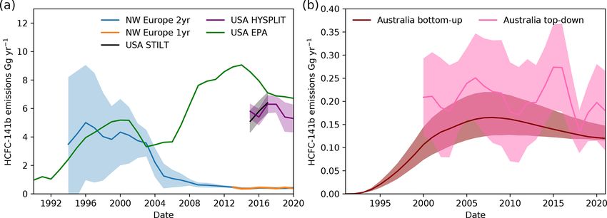
9604                                                                L. M. Western et al.: A rise in global HCFC-141b emissions

the Scripps Institution of Oceanography using Medusa GC–             flask pairs). Monthly semi-hemispheric means were derived
MS technology (Mühle et al., 2010; Trudinger et al., 2016;           using a cosine weighting of site latitude. See Tables S1 and
Mühle et al., 2019). These archived air samples can therefore        S2 and Sect. 2.1 for more details on the measurement sites
be easily integrated with the later AGAGE in situ measure-           and instruments used.
ments.                                                                  Emissions are estimated using an inverse framework
   NOAA estimates of the global mean, remote atmo-                   (Rigby et al., 2014), through minimisation of a cost func-
spheric abundance of HCFC-141b considered here are de-               tion that constrains the emissions growth rate between years.
rived from measurements of air samples pressurised into              A priori, the growth rate was assumed to be zero plus or mi-
paired stainless-steel flasks that have been collected approx-       nus 20 % of the maximum emissions from the EDGAR v4.2
imately weekly at eight remote sites since the earlier 1990s         bottom-up data set (Janssens-Maenhout et al., 2011). Sys-
(see Table S2). The flasks are shipped to Boulder for anal-          tematic uncertainties in the inferred emissions, in addition to
ysis on customised GC–MS instruments (Montzka et al.,                the measurement error, are derived using a Monte Carlo ap-
2015). For deriving continental US emissions from atmo-              proach, which includes errors due to transport, HCFC-141b
spheric measurements, additional flask samples are regularly         lifetime (1 standard deviation uncertainty of 15 % was as-
collected from tall towers (100–400 m a.g.l.; a single flask         sumed, based on SPARC, 2013) and instrument calibration.
per sample, typically) and as profiles from aircraft (6 to 12        The mole fraction growth rate is calculated as the annual
flasks collected at regular altitude intervals in a profile up to    growth rate per month and is smoothed using a Kolmogorov–
8 km a.s.l.) at 17 profiling locations (Hu et al., 2017).            Zurbenko (KZ) filter (Yang and Zurbenko, 2010) using an
                                                                     approximately 18-month window.

2.2     Global emission modelling
                                                                     2.2.2   Consumption-based global emissions modelling
2.2.1    Measurement-based global emissions inference                We estimate emissions using reported global consumption
Global top-down emissions of HCFC-141b, and inferred                 data and an adaptation of the methodology employed by
global mole fractions, are estimated based on atmospheric            Simmonds et al. (2017), where release rates from the re-
mole fraction measurements from either the AGAGE or                  ported bank are estimated to best reproduce the top-down
NOAA network, a 12-box model of global transport and in-             global emissions estimates. We call this approach a top-
verse modelling. The 12-box model simulates annually re-             down-informed bank model. In a given year, i, total emis-
peating advection and diffusion in the global atmosphere             sions to the atmosphere, E, are assumed to come from a com-
(Cunnold et al., 1983; Rigby et al., 2013) and separates the         bination of prompt releases in the year of consumption, C
atmosphere at 30◦ N, the Equator and 30◦ S and at 500 and            (due to losses during production and installation), and emis-
200 hPa. The rate of reaction of HCFC-141b with the hy-              sions from the existing HCFC-141b bank, B, following the
droxyl radical (OH) was taken from Burkholder (2019), and            relationship
global mean OH concentrations were inferred in the box               Ei = f Ci + gBi ,                                          (1)
model based on observations of methyl chloroform (Rigby
et al., 2013). A first-order stratospheric loss was imposed to       where f and g are the prompt and bank release fractions,
give a stratospheric lifetime of 72.3 years. The overall life-       respectively, and remain constant over time. The bank grows
time of HCFC-141b was 9.3 years in the model.                        as
   The measurements from the AGAGE sites that are repre-
                                                                     Bi = (1 − f )Ci−1 + (1 − g)Bi−1 .                          (2)
sentative of background conditions in the semi-hemispheres
of the 12-box model are used to estimate global emissions            We extend this approach by using separate consumption data
(MHD, THD, RPB, SMO and CGO; see Table S1) after                     for Article 5 and non-Article 5 countries, each with very dif-
measurements not representative of background conditions             ferent consumption patterns over time, which allows each to
were removed using a statistical algorithm (O’Doherty et al.,        have their own prompt and bank release fractions (rather than
2001). When measurements are made in the same latitude               the same release fraction, as used in Simmonds et al., 2017).
band using multiple instruments (MHD and THD), the mean                 To derive values for f and g for both Article 5 and non-
value is used. AGAGE monthly mean estimates are based on             Article 5 countries, we use the top-down global emissions es-
one to a few archived air measurements or dozens to hun-             timates and a statistical framework. For this analysis, we only
dreds of in situ measurements. NOAA measurements used                use emissions estimated using AGAGE data, as this measure-
as input to the 12-box model are shown in Table S2. They             ment data set includes measurements of archived air sam-
were also filtered to select only those thought to be represen-      ples, which predate the non-negligible global consumption,
tative of background conditions, eliminating a small fraction        whereas the NOAA data do not. We constrain f and g using
of the entire data record (1.7 % of flask pairs). Results were       the top-down emissions and the relationship in Eq. (1) in a
also eliminated when measured mole fractions in simultane-           Markov chain Monte Carlo framework, which allows uncer-
ously filled flasks differ by more than 0.28 ppt (3.0 % of all       tainties to be propagated throughout. No prior constraint is

Atmos. Chem. Phys., 22, 9601–9616, 2022                                               https://doi.org/10.5194/acp-22-9601-2022
L. M. Western et al.: A rise in global HCFC-141b emissions                                                                 9605

placed on the value of f and g, other than that they must be         Emissions were estimated using a Bayesian Markov chain
between 0 %–100 % with equal prior probability. Under this        Monte Carlo inverse framework (Ganesan et al., 2014; Say
framework, we simultaneously infer consumption in 2021,           et al., 2019) independently each year by scaling an a pri-
which had not been fully reported to UNEP at the time of          ori emissions field and the mole fraction contribution from
writing, considering the uncertainties in the top-down emis-      the model boundary using measurements from Gosan station
sions and release fractions. For 2021, we assume that all con-    averaged into 12-hourly bins. The a priori emissions field
sumption from non-Article 5 countries is less than 1 Gg yr−1      is 1.16 Gg yr−1 for eastern China, 0.13 Gg yr−1 for South
(with equal probability for all values between 0–1 Gg yr−1 )      Korea, 0.17 Gg yr−1 for western Japan and 0.17 Gg yr−1 for
and place no prior constraint on Article 5 consumption, other     North Korea. Emissions were distributed equally in space
than it must be a positive value. We make this assumption as,     over land with a log-normal uncertainty, where the distribu-
under the phase-out schedule, only very minor consumption         tion is described by the shape parameters µ, or log-median
(less than 0.5 % of baseline usage, which is around 0.2 ODP-      value, equal to 0.2, and σ , equal to 0.8. The a priori mole
Gg for all HCFCs, where ODP-Gg is the CFC-11 equiva-              fraction at the model boundary was taken from the AGAGE
lent in terms of ozone-depleting potential) would be expected     12-box model (Rigby et al., 2014). These were assigned a
from non-Article 5 countries. Consumption of HCFC-141b            prior log-normal distribution, with µ equal to 0.004 and σ
in 2020 for non-Article 5 countries was negative; i.e. more       equal to 0.02. In addition to the measurement error, which
HCFC-141b was destroyed than consumed. Therefore, it is           was assumed prior to inference, we estimated the model
reasonable to assume that any consumption, above minor us-        transport error in a normal likelihood, assigning it a log-
age, should only occur in Article 5 countries. As such, it        normal prior distribution of µ equal to 0.2 and σ equal to
is possible to use the estimated 2021 consumption and es-         0.8. The computational domain was divided into 151 basis
timates of release fraction to predict 2021 emissions (with       functions using a quadtree algorithm, and the mole fractions
the propagated uncertainty).                                      at the boundaries were estimated in each cardinal direction
                                                                  (Say et al., 2019; Western et al., 2021). We used a No-U-
2.3     Regional modelling                                        Turn (NUTS) sampler to sample the emissions and bound-
                                                                  ary influence and a slice sampler to sample the model error
Regional emission estimates for east Asia were derived us-        (Salvatier et al., 2016) using 90 000 sampling steps (with an
ing four inverse methods: the Bristol Markov chain Monte          additional 10 000 discarded at the beginning of the sampling
Carlo (MCMC) inversion, Sect. 2.3.1; InTEM, Sect. 2.3.2;          chain). Convergence was checked using a Gelman–Rubin di-
EBRIS, Sect. 2.3.3; and FLEXPART-MIT, Sect. 2.3.4. Re-            agnostic (Gelman and Rubin, 1992) on multiple chains.
gional emissions for northwest Europe (NW Europe) and
Australia were derived using InTEM, Sect. 2.3.2. Regional
emissions for the contiguous United States were derived us-       2.3.2   InTEM
ing the NOAA framework, Sect. 2.3.5. Inverse methods were         The InTEM inversion methodology is described in Manning
run with independent choices to a priori emissions, statistical   et al. (2021). Briefly, the footprint sensitivities were gener-
models, transport set-ups and treatment of measurement data       ated using NAME as described in Sect. 2.3.1 using global
sets, in instances where multiple estimates were performed        UM data. Emission estimates for east Asia were derived us-
for the same region.                                              ing measurement data from Gosan, averaged into 4-hourly
                                                                  time intervals. Prior mean emissions in east Asia were uni-
2.3.1    Bristol MCMC                                             formly distributed over all land areas within the compu-
                                                                  tational domain, with total emissions equal to 50 Gg yr−1
Linear sensitivities of measured mole fraction to emissions
                                                                  and a 1 standard deviation uncertainty equal to 300 % of
(or “footprints”) were derived using the UK Met Office
                                                                  the prior mean emissions. This resulted in the following
NAME model (Jones et al., 2007). Sensitivities were calcu-
                                                                  prior emissions: eastern China 2.6 ± 24.3 Gg yr−1 , South Ko-
lated for a computational domain bounded at 5◦ S and 74◦ N
                                                                  rea 0.3 ± 8.7 Gg yr−1 , western Japan 0.4 ± 9.9 Gg yr−1 and
and 55 and 192◦ E. Meteorology from the UK Met Office
                                                                  North Korea 0.4 ± 9.0 Gg yr−1 .
Unified Model (Met-UM Global, Walters et al., 2014) drives
                                                                     Emission estimates for Europe used measurement data
the transport, which increases in resolution from 0.563 to
                                                                  from Mace Head, Jungfraujoch, Monte Cimone, Tacolne-
0.141◦ longitude and 0.375 to 0.094◦ latitude between 2008–
                                                                  ston and Taunus. For Europe, the footprints were bounded
2020. The temporal resolution remained at 3 h throughout
                                                                  by a computational domain of 10.6 to 79.2◦ N, 98.1◦ W
this period. Around 20 000 particles were released each hour
                                                                  to 39.6◦ E using global UM data nested with higher-
within the NAME model domain, and a measurement was
                                                                  resolution Unified Model meteorology over the United King-
deemed to be sensitive to emissions when a particle was
                                                                  dom and Ireland (UK-V, Tang et al., 2013). The prior emis-
transported within the lowest 40 m above ground level of the
                                                                  sions for countries in NW Europe were 0.1 ± 4.4 Gg yr−1
model domain. Sensitivities were output on a grid of 0.234◦
                                                                  for Belgium and Luxembourg, 1.8 ± 18.1 Gg yr−1 for
longitude by 0.352◦ latitude.
                                                                  France, 1.1 ± 13.5 Gg yr−1 for Germany, 0.3 ± 6.8 Gg yr−1

https://doi.org/10.5194/acp-22-9601-2022                                          Atmos. Chem. Phys., 22, 9601–9616, 2022
9606                                                              L. M. Western et al.: A rise in global HCFC-141b emissions

for Ireland, 0.1 ± 4.8 Gg yr−1 for the Netherlands and             of this optimisation the domain total a priori uncertainty was
1.1 ± 12.7 Gg yr−1 for the UK.                                     determined to be 140 % to 160 % varying from year to year.
   Emissions estimates for Victoria, Tasmania, southern and
southwestern New South Wales, and eastern South Australia          2.3.4   FLEXPART-MIT
are based on measurements at Cape Grim, averaged every
4 h. They are then scaled by population (a factor of 2.6) to       The FLEXPART-MIT inversion is described in Fang et al.
the whole of Australia. Footprints were bound to a compu-          (2019a). The FLEXPART-MIT inversion also used FLEX-
tational domain of 70.0 to 214.7◦ E and 65.0◦ S to 5.0◦ N.         PART to derive footprint sensitivities, but under a differ-
The prior emissions for Australia were 0.4 ± 2.0 Gg yr−1 ,         ent setup to Sect. 2.3.3. In every 3 h interval, 40 000 parti-
distributed by population density.                                 cles were released and tracked backwards for 20 d. Meteo-
   Prior boundary mole fractions at each station were es-          rology was driven by operational ECMWF analysis at 1◦ ×
timated using a fourth-order polynomial fitted to measure-         1◦ global resolution over a global computational domain.
ments that were representative of background air, having lit-         A priori flux fields were spatially uniform over continental
tle influence from populated areas, and refined within the In-     eastern Asia, with no emissions from the ocean. Emissions
TEM framework (see Manning et al., 2021).                          were estimated using a variable-resolution grid. The grid
                                                                   was finest (1◦ × 1◦ ) in eastern China and other eastern Asian
2.3.3   EBRIS
                                                                   countries, and a coarser grid resolution (24◦ × 24◦ ) was used
                                                                   outside this area. A priori emissions estimates of HCFC-141b
A detailed description of the Empa Bayesian Regional Inver-        were 14.5 Gg yr−1 for China (1.5 Gg yr−1 for eastern China)
sion System (EBRIS) is given in Henne et al. (2016). The           and 1.2, 0.27 and 0.27 Gg yr−1 for Japan, South Korea and
method used measurements from the Gosan station, aver-             North Korea, respectively. Prior uncertainty was arbitrarily
aged every 3 h, to derive emissions. Footprint sensitivities       set to 1000 % of the a priori estimate, which assumed a spa-
for east Asia were derived using the FLEXPART transport            tial correlation length of 300 km. The background mole frac-
model (Pisso et al., 2019), which was driven by operational        tions were estimated in 7 d periods. Model–measurement un-
ECMWF analysis meteorology with 1◦ × 1◦ resolution, re-            certainty for each 24 h averaged observation was estimated
ducing to 0.2◦ × 0.2◦ resolution for northeastern China (105       using the quadratic sum of 1 % of the baseline value (as a
to 125◦ E and 30 to 50◦ N). In each 3 h interval, 50 000 parti-    measure of baseline uncertainty), the measurement repeata-
cles were released and tracked backward for 10 d. Footprints       bility and the standard deviation of the 24 h variability (as a
were derived for a large northern hemispheric domain at a          measure of the model–data mismatch uncertainty).
resolution of 0.125◦ × 0.125◦ and a particle sampling height          The inverse framework utilises a Bayesian framework us-
of 100 m.                                                          ing an analytical solution to a normal likelihood and prior
   Inversions were carried out independently for average an-       (Stohl et al., 2009) for each year.
nual emissions. The inversion grid (state vector) was limited
to the domain 80 to 140◦ E and 20 to 60◦ N. Grid resolu-           2.3.5   NOAA
tion was inversely proportional to the average footprint, with
smaller grid cells (0.125◦ × 0.125◦ ) close to the measure-        The NOAA inversion framework was first presented in Hu
ment site and large grid cells (8◦ × 8◦ ) away from the mea-       et al. (2015) and is used to derive US emissions for a num-
surement site. Approximately 500 grid cells were included          ber of ozone-depleting substances and their substitutes (Hu
in the inversion grid, depending on the data coverage of indi-     et al., 2016, 2017). A similar methodology was used here to
vidual years.                                                      derive US emissions of HCFC-141b for 2015–2020. A total
   Baseline concentrations were estimated using the robust         of six ensemble inversions with identical a priori emission
estimation of baseline signal (REBS) method (Ruckstuhl             fields were conducted for deriving US HCFC-141b emis-
et al., 2012) applied to the observations at Gosan. Every 2        sions (three approaches to estimate background mole frac-
weeks baseline concentrations were part of the state vector        tion using two transport models). The US a priori HCFC-
and were optimised during the inversion step.                      141b emissions were 4.1 Gg yr−1 and were scaled by popu-
   The same a priori emissions were assigned for each              lation density to generate 1◦ × 1◦ a priori emissions. Prior
year in the inversion. Homogeneous a priori distribu-              uncertainties were estimated by maximum likelihood esti-
tions were prescribed in each of the seven focus regions           mation (Michalak et al., 2005; Hu et al., 2015). Footprints
(western China, 6.3 Gg yr−1 ; eastern China, 6.7 Gg yr−1 ;         were simulated by two transport models, the Hybrid Single-
North Korea, 0.1 Gg yr−1 ; South Korea, 1.0 Gg yr−1 ; west-        Particle Lagrangian Integrated Trajectory Model (HYSPLIT)
ern Japan, 2.0 Gg yr−1 ; eastern Japan, 0.6 Gg yr−1 ; Taiwan,      for 2015–2020 and the Stochastic Time-Inverted Lagrangian
0.2 Gg yr−1 ).                                                     Transport (STILT) model for 2015–2017. The HYSPLIT
   The a priori covariance and data-mismatch covariance            model was run with 500 particles back in time for 10 d
were estimated using a log-likelihood optimisation of param-       and driven by the North American Mesoscale Forecast Sys-
eters describing the covariance (Henne et al., 2016). As part      tem (NAMS) with 40 sigma-pressure levels and 12 km hor-

Atmos. Chem. Phys., 22, 9601–9616, 2022                                             https://doi.org/10.5194/acp-22-9601-2022
L. M. Western et al.: A rise in global HCFC-141b emissions 9607
izontal resolution over the contiguous United States. The where σi is the 1-sigma posterior uncertainty derived from
NAMS meteorology was nested with a global meteorological each inversion; σs denotes the 1-sigma spread of the posterior
field, the US National Centers for Environmental Prediction emissions derived from all six inversions.
(NCEP) 0.5◦ Global Data Assimilation System (GDAS0.5)
with 55 sigma-pressure levels (before June 2019) and the
3 Results and discussion
NCEP 0.25◦ Global Forecast System (GFS0.25) forecast
model with 55 sigma-pressure levels (after June 2019). The 3.1 Global mole fraction and emissions
STILT simulation was also run with 500 particles back in
time for 10 d. It was driven by the Weather Research and As expected from the Montreal Protocol-mandated HCFC
Forecasting Model (WRF) with 10 km resolution over North phase-out schedule, global emissions of HCFC-141b had
America and 40 km resolution outside of North America. been declining since 2012 (Montzka et al., 2015; Simmonds
Three different approaches were used to derive back- et al., 2017; Engel and Rigby, 2019). However, since 2017,
ground HCFC-141b mole fractions for measurements made an increase in emissions is evident from recent changes in
in the United States (see details described in Hu et al., the distribution and global mean mole fraction of HCFC-
2017, 2021). All three approaches were first based on a 3D 141b. The growth rate of the global mole fractions had con-
background field (as a function of time, latitude and altitude) tinuously slowed since 2012, and the global mole fractions
constructed from atmospheric observations far away from started to decline during 2017 (Fig. 3a and b for AGAGE
emission sources, i.e. those made over the Pacific Ocean and and NOAA, respectively). Such a slow-down and decline are
Atlantic Ocean basins near Earth’s surface and in the free expected as emissions decrease and HCFC-141b present in
troposphere above North America. In the first approach, we the atmosphere is destroyed by reactions with the OH radical
estimated the background mole fraction associated with each and photolysis in the stratosphere. Since 2018, however, the
measurement made in the United States by assigning mole rate of decline in global mole fraction slowed and, as of 2019,
fractions from this 3D background field based on the sam- annual mean growth rates are positive again. This increase is
pling time, latitude and altitude for measurements made in likely being driven by increased emissions in the Northern
the United States. In our second approach, we considered air Hemisphere, as the increase in the growth rate in the North-
back-trajectories for individual measurements made in the ern Hemisphere leads that in the Southern Hemisphere in re-
United States. We estimated the time and location of each cent years, just as it did in earlier periods when the global
particle exiting the planetary boundary layer of the contigu- HCFC-141b growth rate and emissions were rapidly increas-
ous United States based on its back-trajectories and assigned ing (e.g. 1992–1996 and 2009–2012). As of 2019 there is
the mole fraction from the 3D background at the exiting time a growing difference between the observed mole fraction in
and location. The third background estimate for each mea- the Northern Hemisphere and Southern Hemisphere (mean
surement in the United States is an average of 500 back- difference of 1.8 ppt in 2018 and 2.2 ppt in 2021).
ground estimates based on the 500 back-trajectories. In this Using AGAGE and NOAA measurements, we show that
third approach, we considered possible biases in transport emissions of HCFC-141b started to increase again in 2018,
simulations and lack of mole fraction information in the plan- despite the reported reduction in global dispersive produc-
etary boundary layer of the United States, because some par- tion and consumption expected from the Montreal Protocol
ticles remained in the planetary boundary layer of the United control schedules (Figs. 1 and 4a). Aggregated emissions
States after 10 d of running the transport model backward in from 2017 to 2021 have increased by an additional 4.4 ± 1.9
time. Thus, we applied a likely bias correction to the back- (AGAGE) or 7.5 ± 0.5 Gg (NOAA), an average linear in-
ground derived from the second approach by comparing ob- crease at a rate of 1.1 ± 0.2 Gg yr−1 per year (AGAGE) or
served mole fractions with estimated background mole frac- 1.6 ± 0.1 Gg yr−1 per year (NOAA). This assumes that all
tions for a subset of observations with minimal surface emis- uncertainty is only due to the random error component of
sion influence, i.e. summed footprint over populated areas the emissions estimates (i.e. systematic uncertainty causes
(areas with more than 10 persons per square kilometre) less an offset in emissions and does not impact year-to-year vari-
than 0.1 ppt (pmol m−2 s−1 )−1 . The final annual US emis- ability). Note that Fig. 4 shows the uncertainty due to the
sions were reported as the ensemble mean and uncertainties combined random and systematic error components.
from the six inversions. The reported uncertainties are a 1- To understand this reversal, we estimate global emissions
sigma uncertainty (σt ) calculated as of HCFC-141b using reported consumption data by adapting
v the approach taken by Simmonds et al. (2017), as detailed
u
u 1X 6 in Sect. 2.2.2. We estimate the prompt release fraction to be
σt = tσs2 + σ 2, (3) 24 (17–31) % and 37 (36–39) % of the annual consumption
6 i=1 i
for Article 5 and non-Article 5 countries, respectively (68 %
uncertainty interval). Our estimated annual bank release frac-
tion is 3.6 (3.0–4.2) % from the remaining bank and 2.8 (1.9–
3.9) % for Article 5 and non-Article 5 countries, respectively,
https://doi.org/10.5194/acp-22-9601-2022 Atmos. Chem. Phys., 22, 9601–9616, 20229608 L. M. Western et al.: A rise in global HCFC-141b emissions Figure 3. HCFC-141b global and semihemispheric mole fraction (top), growth rate (middle) and north–south interhemispheric difference (bottom) derived from AGAGE (a) and NOAA (b) measurements. Lines show mole fractions in each semihemisphere derived with the 12-box model using available data, whilst the dots represent the observations as monthly means of background measurements from all sites within each semihemisphere for each network. The grey shading shows the 1 standard deviation estimate in the global mean mole fraction. The north–south interhemispheric difference is a 12-month rolling mean. Figure 4. (a) HCFC-141b global emissions derived from AGAGE and NOAA measurements and derived from reported consumption data and estimated emission release fractions, where consumption has been predicted for 2021, assuming consumption in non-Article 5 countries is less than 1 Gg yr−1 and no constraints on Article 5 consumption. (b) A breakdown of HCFC-141b global emissions from Article 5 and non-Article 5 countries using the consumption-based emissions estimate, where 2021 consumption has been estimated from the top-down emissions data. and is assumed to be unchanged since 1989. Simmonds et al. rive the respective emissions using the top-down-informed (2017) used an aggregated HCFC-141b prompt release frac- bank model. Under the constraints of the top-down-informed tion of 34.5 ± 4.0 %, along with a bank release fraction of bank model, we are able to estimate the necessary consump- 2.2 %. Our estimated released fractions thus broadly agree tion needed to produce the observed top-down emissions in with that used by Simmonds et al. (2017) and that previ- 2021, which has not yet been fully reported. This uses the re- ously estimated for closed foams containing CFC-11 (TEAP, ported consumption until 2020 and the estimated emissions 2019), which is 25 %–35 % for the prompt release fraction rate from the bank to estimate the needed 2021 consumption and 1.5 %–4.2 % for the bank release fraction. Using the re- to reproduce the top-down emissions estimate. This analysis, ported consumption and estimated release fraction, we de- under the constraints of the model, suggests that consump- Atmos. Chem. Phys., 22, 9601–9616, 2022 https://doi.org/10.5194/acp-22-9601-2022
L. M. Western et al.: A rise in global HCFC-141b emissions                                                                9609

tion likely rose between 2020 and 2021, from 39 Gg yr−1 in       emission trends in China to other developing countries, and
2020 to 67 (28–95) Gg yr−1 in 2021. This consumption esti-       there is likely considerable uncertainty and variation in the
mate for 2021 is very uncertain due to the uncertainty in the    life cycle of appliances containing HCFC-141b foam and
top-down-derived emissions, and so a decline in global emis-     their disposal practices.
sions, and thus decline in consumption, cannot be excluded.         The top-down-informed bank model neglects emissions
Increasing consumption between 2017–2020 is not possible         from feedstock and other so-called non-dispersive produc-
in this model, due the constraints imposed by the reported       tion. A typical emissions factor associated with fluorochem-
production and bank behaviour. An alternative conclusion         ical production is around 4 % (IPCC, 2019). If applied
that could be drawn from this analysis, under the assump-        to global feedstock production, additional feedstock-related
tion that reported consumption should decrease in 2021, is       emissions would be 0.5 Gg yr−1 between 2017–2020, not
that the emissions rate from the bank has increased in more      enough to explain the global increase, with no increasing
recent years, meaning that the inferred emissions rate, which    trend. Emissions factors from individual production facili-
is constant in time, is no longer representative and cannot      ties may vary considerably (0.1 %–20 %, 95 % uncertainty,
adequately model emissions.                                      IPCC, 2019). A universal feedstock production leakage rate
   Figure 4a shows a comparison of the top-down atmo-            of 20 % in 2020 compared to 0.1 % in 2017 would be needed
spheric measurement-derived emissions, using the 12-box          to explain the observed global increase in emissions. This
model (and without using information about reported con-         would result in an additional 3.0 Gg yr−1 of emissions, com-
sumption), and the emissions estimated using the top-down-       pared to a mean global increase in the NOAA and AGAGE
informed bank model. Although these estimates are unique,        estimates of 3.0 ± 1.2 Gg yr−1 during the same period. A
they are not independent due to both top-down estimates us-      sustained rapid deterioration in feedstock production losses
ing the same methodology to derive emissions using AGAGE         since 2017 seems an unlikely scenario to explain the global
and NOAA measurements and the dependence of the top-             increase in emissions.
down-informed bank model on the estimates using AGAGE               In the following section we turn to regional emissions es-
measurements. Figure 4b shows a breakdown of the mean            timates of HCFC-141b, where observations are available, to
emissions from non-Article 5 and Article 5 countries under       further diagnose the driver behind the global rise.
the top-down-informed bank model using reported consump-
tion data and assumptions inherent in the model, where 2021      3.2   East Asian emissions
consumption has been estimated. This imposes that all con-
sumption in 2021 (over a maximum of 1 Gg yr−1 ) must come        Atmospheric measurement-based emissions estimates for
from Article 5 countries (see Sect. 2.2.2).                      east Asia are based on four different inverse methods us-
   The timing of this increase in HCFC-141b emissions is         ing measurements from Gosan station, South Korea (see
nearly coincident with the rapid post-2018 global decline in     Sect. 2.1), and are combined into a single estimate using
CFC-11 emissions (Montzka et al., 2021), which may sug-          Monte Carlo sampling. These results provide emissions es-
gest that the enhanced apparent use and production of CFC-       timates for South Korea, North Korea and two regions that
11 during 2012–2018, which was likely used for foam pro-         we denote eastern China (which includes the provinces of
duction, may have transitioned to HCFC-141b instead of           Anhui, Beijing, Hebei, Jiangsu, Liaoning, Shandong, Shang-
transitioning to newer replacements. An explanation for the      hai, Tianjin and Zhejiang) and western Japan (which includes
recent rise in global HCFC-141b emissions is, however, fur-      the regions Chūgoku, Kansai, Kyūshū and Okinawa, and
ther complicated by a lack of understanding of the time-         Shikoku), as measurements at Gosan have little sensitivity
dependent changes in emissions from the existing HCFC-           to emissions in western China or eastern Japan.
141b bank. Wang et al. (2015) suggest that HCFC-141b                Emissions of HCFC-141b from eastern China show an
emissions in China are expected to peak in 2025–2027,            increase in emissions from 3.7 (1.8–4.8) Gg yr−1 in 2008
15 years after peak consumption in China. This is attributed     to 6.8 (3.7–9.4) Gg yr−1 in 2020 and an increase of 1.0
to the release of HCFC-141b from foams during the disposal       (−2.9, 3.8) Gg yr−1 between 2017–2020. The 2017–2020 in-
of insulated refrigerators and electric water heaters at their   crease in eastern China could account for around a third of
end of life around 15 years after peak consumption. If such a    the global increase over the same period (3.0 ± 1.2 Gg yr−1 ,
pattern predicted in China is applied to all developing coun-    NOAA and AGAGE mean), but given the large uncertain-
tries, peak emissions from all developing countries would be     ties this could explain all or none of the global increase. The
expected around 2026–2027, 15 years after their peak con-        mean emissions of the inverse frameworks (Fig. 5) gener-
sumption in 2011–2012, and could perhaps explain the ob-         ally agree well with bottom-up inventory estimates for China
served emissions increase. However, a study in Lahore, Pak-      (Fang et al., 2018) scaled down to the eastern China region by
istan, showed that HCFC-141b emissions due to waste and          population or gross domestic product from emissions from
disposal of HCFC-141b-containing refrigerators fell between      the whole of China (the range is shown by the orange shading
2005 and 2013 (Ul-Haq et al., 2016). It may therefore not        in Fig. 5), given the uncertainties in the top-down modelling
be appropriate to extrapolate the bottom-up-predicted bank       and the uncertainties likely present in the bottom-up model

https://doi.org/10.5194/acp-22-9601-2022                                        Atmos. Chem. Phys., 22, 9601–9616, 2022
9610                                                             L. M. Western et al.: A rise in global HCFC-141b emissions

(which were not given in the study). The top-down-derived         slightly between 2015 and 2017, with 5.5 ± 0.6 in 2015 and
emissions trend is also supported by the projected emissions      6.4 ± 0.7 Gg yr−1 in 2017. The HYSPLIT-NAM model esti-
of Wang et al. (2015), although emissions projected by Wan        mate suggests that emissions remain unchanged in 2018 at
et al. (2009) were expected to peak in 2018. If the bottom-       6.3 ± 0.6 and fall to 5.3 ± 1.0 Gg yr−1 in 2020. Bottom-up
up-predicted emissions by Wang et al. (2015) and Fang et al.      emissions estimates by the U.S. Environmental Protection
(2018) come to fruition, HCFC-141b emissions from China           Agency (EPA, 2021) over the same period (Fig. 6a) sug-
will continue to rise until the mid-2020s. Our results pre-       gest that emissions fell from 8.6 in 2015 to 7.1 Gg yr−1 in
sented here for eastern China contrast with top-down esti-        2017 to 6.7 Gg yr−1 in 2020. The reason for the discrep-
mates presented for the whole of China in previous studies        ancy in the trend between the top-down and bottom-up es-
(Fang et al., 2019b; Yi et al., 2021), which suggest a contin-    timates in 2015–2016 is unclear; however both show only
ual fall in emissions.                                            small changes in emissions between 2017–2020. The NOAA
   Emissions from South Korea (around 1–3 Gg yr−1 ) are           top-down estimates are 10 %–40 % smaller than the U.S.
smaller than from eastern China, and it is uncertain whether      EPA bottom-up estimates (assuming that the non-contiguous
they are increasing or decreasing. Emissions from western         states and territories are not responsible for the discrepancy).
Japan and North Korea are even smaller (generally less than          Consumption of HCFCs in the United States from 2002
around 1 Gg yr−1 ). Japan, in contrast to other east Asian        to 2003 fell to around half and has continued to decline.
countries, legislates the removal and destruction of HCFC         The U.S. EPA emission estimate suggests peak emissions
refrigerants and HCFCs in foams within appliances through         many years after a peak consumption, different from what the
the Home Appliance Recycling Act (Hotta et al., 2016).            NW European top-down emissions show and more similar to
                                                                  bottom-up projections for China. The reason for a slowing in
3.3    Northwestern European emissions
                                                                  the decline of emissions since 2017 is not fully clear, but the
                                                                  bottom-up model suggests that it may be due to post-disposal
Emissions for northwestern Europe (Belgium, France, Ger-          emissions from polyurethane foams used for domestic refrig-
many, Ireland, Luxembourg, the Netherlands and the United         erator and freezer insulation, occurring during the 26 years
Kingdom) were estimated using the InTEM inversion sys-            following disposal (EPA, 2021). This assumes that domestic
tem, based on measurements from Mace Head in Ire-                 refrigerators and freezers have a lifetime of 14 years and that
land, starting in 1994, with additional measurements from         the leakage post-disposal (2 %) is higher than that during the
Jungfraujoch in Switzerland from 2008, Monte Cimone in            appliance lifetime (0.25 %). In the United States, a gradual
Italy from 2012, Tacolneston in the UK from 2012 and              increase in HCFC-141b emissions due to the disposal of do-
Taunus in Germany from 2013. NW Europe sees a sharp               mestic refrigerants following a peak in consumption may be
fall in emissions after 2003, Fig. 6a, from 3.6 ± 0.9 in 2003     occurring, much like that predicted to occur in China, offset-
to 2.2 ± 1.0 Gg yr−1 in 2004 and then 1.3 ± 0.9 Gg yr−1 in        ting reductions in other banks. Unlike the European Union,
2005, with timing consistent with the phase-down of HCFC          which mandates destruction of HCFC-141b within refriger-
production in those countries. Emissions have steadily fallen     ator foams, the U.S. EPA’s Responsible Appliance Disposal
since, reaching 0.4 ± 0.1 Gg yr−1 in 2020. Emissions from         (RAD) Program is voluntary. This may explain different US
individual countries are presented in the Supplement.             and European HCFC-141b emission patterns, despite similar
   Emissions in NW Europe peak coincidentally with high           consumption patterns.
consumption in developed countries. The European Union’s
Regulation (EC) 1005/2009 (and similar legislation in the         3.5   Australian emissions
UK) requires that appliance foam insulation controlled un-
der the Montreal Protocol is recovered at disposal to be re-      Top-down HCFC-141b emissions estimates using InTEM
cycled or properly destroyed. Therefore we expect relatively      show that emissions in Australia have remained largely con-
low end-of-life emissions in NW Europe, in comparison to          stant from 2000 to 2021, perhaps showing a slight decline
the emissions rates in China, and our results provide evidence    (Fig. 6b).
that such legislation has, likely, been effective.                   Australia has not produced or exported HCFC-141b, and
                                                                  therefore HCFC-141b consumption is governed by imports,
3.4    Contiguous US emissions
                                                                  assuming that no significant stockpiling for later use oc-
                                                                  curred. Australian HCFC-141b imports/consumption com-
Top-down emissions estimates for the contiguous United            menced in the early 1990s, reaching 0.8–0.9 Gg in 1999 and
States from 2015 to 2020 (Fig. 6a) are derived from mea-          then declining to zero by 2012, well ahead of the mandated
surements made by NOAA’s North American sampling net-             HCFC phase-out schedule (Dunse et al., 2021). From 1991
work (see Sect. 2.3.5 and 2.1) using two atmospheric trans-       to 2012, Australian HCFC-141b imports totalled 7.8 Gg.
port models and the NOAA inversion framework (Sect. 2.3.5,           Assuming that emissions have therefore only come from
Hu et al., 2016). Taking an average of the two top-down           the bank, and using the emissions factor derived for non-
estimates for the United States, emissions likely increased       Article 5 countries from Sect. 3.1, we derive a bottom-up

Atmos. Chem. Phys., 22, 9601–9616, 2022                                            https://doi.org/10.5194/acp-22-9601-2022
L. M. Western et al.: A rise in global HCFC-141b emissions 9611
Figure 5. Emissions estimates for east Asia. (a) Combined top-down emissions from four inversion frameworks for eastern China with
their 68 % uncertainties (blue). Bottom-up emissions estimates for eastern China (orange) estimated by scaling down the Fang et al. (2018)
estimate for the whole of China by either population or gross domestic product to eastern China. The shading shows the range between these
two metrics for scaling. (b) Top-down estimates for South Korea, western Japan and North Korea.
Figure 6. (a) Annual InTEM emissions from northwestern Europe using a 2-year inversion period (blue) or only a single year (orange) and
from the contiguous United States using two transport models, HYSPLIT (purple, 2015–2020) and STILT (black, 2015–2017). Bottom-up
estimates for the United States are shown in green. (b) Annual InTEM emissions for Australia (pink) and bottom-up emissions estimated
using consumption data (dark red).
emissions estimate based on consumption in Australia. The HCFC-141b declined. However, the trend reversed and emis-
bottom-up model likely underestimates the emissions re- sions increased by 3.0 ± 1.2 Gg yr−1 or 6 % from 2017 to
lease rate because prompt emissions, which we assume to 2021, even though reported production for dispersive uses
include emissions during installation and immediate usage, continued to decrease. This timing is similar to a decline
have not been included. The top-down and bottom-up esti- in global emissions of CFC-11, the ozone-depleting sub-
mates for Australia generally agree, given the large uncer- stance replaced by HCFC-141b for foam blowing, following
tainties. Australia has no laws to mandate the destruction of a period of increasing global CFC-11 emissions, of which
HCFCs within appliance-insulating foams at disposal. How- 60 ± 40 % could be attributed to eastern China (Park et al.,
ever, there is no obvious increase in HCFC-141b emissions 2021). Due to a current incomplete understanding of the size
in Australia in recent years due to an increase in the rate of and behaviour of the global HCFC-141b bank, it is uncertain
emissions from foam-containing appliances when they reach whether the emission rise is due to unreported production for
their end of life (within uncertainties). dispersive uses, as suggested by a simple bottom-up model
constrained by measurement-derived emissions; due to emis-
sions at the end of life of foam-containing products; or due
4 Conclusions
to a combination thereof.
An increase due to emissions from the bank is suggested
For 5 years after the reported 2012 peak in HCFC-141b pro-
by bottom-up emissions projections for China due to the dis-
duction, global emissions of the ozone-depleting substance
https://doi.org/10.5194/acp-22-9601-2022 Atmos. Chem. Phys., 22, 9601–9616, 20229612 L. M. Western et al.: A rise in global HCFC-141b emissions
posal of appliances containing HCFC-141b foam, without able in the Supplement. The NAME model and InTEM mod-
destroying the HCFC-141b. However, according to bottom- els are available for research purposed via request to the UK
up and top-down estimates, emissions from China alone can- Met Office (enquiries@metoffice.gov.uk) or on request to Alis-
not fully explain the global rise. This pattern of bank-related tair J. Manning or Alison L. Redington. The FLEXPART model
emissions years after peak consumption may not apply to is available from https://www.flexpart.eu (Pisso et al., 2019). The
EBRIS algorithm is available from https://doi.org/10.5281/zenodo.
other developing countries. Emissions in the United States
1194642 (Henne, 2018). The Bristol MCMC inversion code is
and Australia, where there are no strict requirements in place available at https://github.com/ACRG-Bristol/acrg (last access: 20
for the destruction of HCFCs upon appliance disposal, do July 2022) (https://doi.org/10.5281/zenodo.6834888, Rigby et al.,
not show evidence of declining, or increasing, emissions 2022). The code for the FLEXPART-MIT inversion is available
in recent years. This contrasts with the European Union, from Xuekun Fang upon request. The code for the NOAA inversion
which mandates more complete HCFC destruction upon dis- is available from Lei Hu upon request.
posal, where emissions have decreased continuously since
the phase-out of consumption began. A lack of declining
emissions in the United States and Australia may support Supplement. The supplement related to this article is available
the argument that a change in emissions rates from the foam online at: https://doi.org/10.5194/acp-22-9601-2022-supplement.
banks after the disposal of foam-containing appliances is
driving the rise in emissions.
Emissions of HCFC-141b feedstock is unlikely to be the Author contributions. LMW led the writing of the manuscript
cause of the global increase, unless emission rates during with contributions from ALR, AJM, CMT, LH, SH, JM, SR, MKV,
production have rapidly increased, from near-zero losses to SAM, MR, and all other coauthors. LWM, ALR, AJM, CMT, LH,
SH and XF performed inverse modelling. LJMK provided data on
around a fifth of production. The amount and fate of HCFC-
reported consumption and production. DSG provided bottom-up
141b produced as a byproduct are unknown, and we have
US HCFC-141b emissions. LJMK, CT and DSG provided input
no evidence to suggest that this pathway leads to significant on HCFC-141b uses, the behaviour of the banks and appliance life
emissions or would have changed substantially since 2017 in cycles. BD provided data and analysis on Australian consumption
a way that could explain the global emission increase. and emissions. JM assisted with data curation. JA, AE, PJF, CMH,
The regional-scale emissions considered here only account PBK, MM, SAM, JM, SO’D, HP, SP, SR, PKS, DS, RS, TS, CS,
for around 30 % of global emissions in 2020. The combined KMS, IV, MKV and DY provided measurement data. SAM, RGP,
regional-scale emissions decreased by 2.3 ± 4.6 Gg yr−1 be- MR and RFW provided oversight to the work and the measurement
tween 2017–2020, compared to a mean global increase in networks.
the NOAA and AGAGE estimates of 3.0 ± 1.2 Gg yr−1 dur-
ing the same period. It seems likely that a substantial recent
increase in emissions is coming from regions that we have Competing interests. The contact author has declared that none
not studied here. of the authors has any competing interests.
We cannot demonstrate a conclusive driver behind the
2017–2021 increase in global emissions, given the infor-
Disclaimer. Publisher’s note: Copernicus Publications remains
mation available. A better understanding of the behaviour
neutral with regard to jurisdictional claims in published maps and
of the HCFC-141b bank and its expected emissions, and institutional affiliations.
more widespread measurement-based emissions monitoring,
would aid in understanding the causes for the current rise in
HCFC-141b emissions. Special issue statement. This article is part of the special issue
“Atmospheric ozone and related species in the early 2020s: latest
results and trends (ACP/AMT inter-journal SI)”. It is a result of the
Code and data availability. AGAGE data are available at http: 2021 Quadrennial Ozone Symposium (QOS) held online on 3–9
//agage.mit.edu/data/agage-data (last access: 17 March 2022) and October 2021.
https://doi.org/10.15485/1841748 (Prinn et al., 2022). NOAA at-
mospheric observations are available at the NOAA atmospheric
observations are available at the NOAA/GML website (updated Acknowledgements. We thank the site operators for their con-
from Montzka et al., 2015; https://gml.noaa.gov/hats/, last ac- tinued support to maintain the measurements at the AGAGE and
cess: 6 April 2022). Measurements of archived air samples NOAA stations and the NOAA and CIRES personnel for techni-
are available in the Supplement. The 12-box model and the cal and logistical support of facilitating the collection of tower and
inverse method used to quantify emissions are available via aircraft samples throughout North America. We thank Arlyn An-
GitHub, https://github.com/mrghg/py12box (last access: 20 July drews for providing the WRF-STILT footprints and Nada Derek
2022), https://github.com/mrghg/py12box_invert (last access: 20 for Cape Grim data analysis. We greatly thank Phil DeCola for
July 2022), and Zenodo (https://doi.org/10.5281/zenodo.6857447, supporting some of NOAA’s inverse modelling analyses. The
Rigby and Western, 2022a, https://doi.org/10.5281/zenodo.685779, NASA Upper Atmosphere Research Program supports AGAGE (in-
Rigby and Western, 2022b). Inputs to this model are avail-
Atmos. Chem. Phys., 22, 9601–9616, 2022 https://doi.org/10.5194/acp-22-9601-2022You can also read