A Unified Statistical Learning Model for Rankings and Scores with Application to Grant Panel Review
←
→
Page content transcription
If your browser does not render page correctly, please read the page content below
A Unified Statistical Learning Model for Rankings and
                                                 Scores with Application to Grant Panel Review

                                          Michael Pearce                                                                   mpp790@uw.edu
                                          Department of Statistics
                                          University of Washington
                                          Seattle, WA 98195-4322, USA
                                          Elena A. Erosheva                                                            erosheva@uw.edu
arXiv:2201.02539v1 [stat.ME] 7 Jan 2022

                                          Department of Statistics, School of Social Work, and the Center for Statistics and the Social Sci-
                                          ences
                                          University of Washington
                                          Seattle, WA 98195-4322, USA

                                                                                        Abstract
                                              Rankings and scores are two common data types used by judges to express preferences
                                              and/or perceptions of quality in a collection of objects. Numerous models exist to study
                                              data of each type separately, but no unified statistical model captures both data types si-
                                              multaneously without first performing data conversion. We propose the Mallows-Binomial
                                              model to close this gap, which combines a Mallows’ φ ranking model with Binomial score
                                              models through shared parameters that quantify object quality, a consensus ranking, and
                                              the level of consensus between judges. We propose an efficient tree-search algorithm to
                                              calculate the exact MLE of model parameters, study statistical properties of the model
                                              both analytically and through simulation, and apply our model to real data from an in-
                                              stance of grant panel review that collected both scores and partial rankings. Furthermore,
                                              we demonstrate how model outputs can be used to rank objects with confidence. The
                                              proposed model is shown to sensibly combine information from both scores and rankings
                                              to quantify object quality and measure consensus with appropriate levels of statistical
                                              uncertainty.
                                              Keywords: preference learning, score and ranking aggregation, Mallows’ model, A*
                                              algorithm, peer review

                                          1. Introduction
                                          Preference data is common to our world: Citizens express preferences through voting in
                                          elections, critics rank movies when creating annual top-10 lists, judges score figure skaters
                                          in the Olympics using numerical scales, wine critics use Likert scales with words such as
                                          “mediocre” to rate wines, consumers use stars to convey the quality of a product, and
                                          so on. As can be seen in these examples, preferences appear in different forms: most
                                          commonly as rankings or scores. Rankings denote a relative order of objects from best
                                          to worst, potentially allowing ties; ranks refer to the specific place of each object in the

                                          ©2022 Michael Pearce and Elena A. Erosheva.
                                          License: CC-BY 4.0, see https://creativecommons.org/licenses/by/4.0/.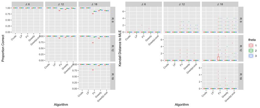
Pearce and Erosheva

ranking. Scores are numerical values given to objects to denote their quality. Scores provide
more granular information than rankings through the relative distance between scores
and the rankings they induce. A number of existing models (Mallows, 1957; Fligner and
Verducci, 1986; Rost, 1988) have been studied to model rankings and scores individually.
In these models, a natural goal is to aggregate preferences into a consensus ranking, which
expresses the overall preferences of those providing the rankings, whom we call judges.
Statistical models may additionally incorporate information regarding the uncertainty of
those rankings, or the level of global or local consensus between the judges.
    When both rankings and scores are available, incorporating the additional information
may improve accuracy of preference aggregation. Rankings and scores arise simultane-
ously in a number of scenarios. For example, in peer review, judges may score proposals
numerically and subsequently rank their top few favorites. Another example arises dur-
ing information retrieval when relevancy criteria from different sources and types—such as
from an algorithmic database search for relevant documents or from human judgment—
are available (Hsu and Taksa, 2005). In the former example, judges provide both kinds of
information, while in the latter, one system may provide rankings and another may pro-
vide scores. Either way, it is unclear how the information from each preference data type
should be utilized. Renda and Straccia (2003) suggest that neither ranking or score data is
uniformly better than the other when analyzed alone (in the context of metasearch), and
many authors have argued that using both is better (Belkin et al., 1995; Macdonald and
Ounis, 2009; Lee, 1997; Balog et al., 2012). To incorporate both sources of information,
conversion of data from one type to another is common (Hsu and Taksa, 2005; Bhamidipati
and Pal, 2008; Li et al., 2009). These methods will be discussed in Section 2. Yet, to the
best of our knowledge, there are no statistical models that combine information from both
rankings and scores without data conversion. Although convenient, data conversion may
result in a loss of information or affect results depending on the chosen conversion process,
which is suboptimal.
    In this paper, we propose a unified model to capture information from both rankings
and scores when applied to a finite collection of objects. Model parameters can be used
to quantify both the absolute and relative qualities of the objects, identify a consensus
ranking, and measure the strength of consensus using an existing metric in the literature.
We formulate exact and approximate algorithms to find maximum likelihood estimators of
the model parameters and demonstrate regimes in which each may be useful. In addition
to simulation studies, we apply the model to real data from grant panel review in which
scores and rankings were collected from the same judges. We show how the estimated
parameters can be used to learn the rank ordering of grant proposals and the associated
statistical uncertainty to make funding decisions.
    The rest of this paper is organized as follows. After discussing related work in Section 2,
we state our proposed model and describe its statistical properties in Section 3. We propose
exact and approximate frequentist estimation algorithms in Section 4, and compare their
speed and accuracy on simulated data in Section 5. We illustrate the model application

                                              2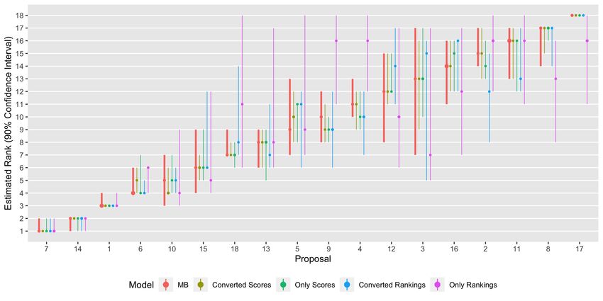
A Unified Model for Rankings and Scores

on real ranking and score data collected during the Fall 2020 grant panel review cycle at
the American Institute of Biological Sciences (AIBS) in Section 6. We conclude with a
discussion in Section 7.

2. Related Work
A variety of methods can be used to aggregate ranking data alone, such as the Plackett-
Luce, Bradley-Terry, and Mallows’ models (Plackett, 1975; Bradley and Terry, 1952; Mal-
lows, 1957). The latter model and its extensions have been particularly well-studied in
recent decades. In a seminal work, Fligner and Verducci (1986) state statistical qualities of
the Mallows’ θ and φ models, which are based on the correlation coefficients of Spearman
(1904) and Kendall (1938), respectively. The Mallows’ φ model has received particular
attention as a natural fit in many ranking applications. Henceforth referred to simply as
the Mallows’ model, it is a location-scale probability distribution that measures distance
between rankings using Kendall’s τ , or the minimum number of adjacent swaps between
objects needed to convert one ranking into another. Many extensions exist, such as the
Generalized Mallows’ model that permits unique scale parameters at each ranking level
(Fligner and Verducci, 1988) and the Infinite Generalized Mallows’ model to aggregate
rankings over infinite collections of objects (Meila and Bao, 2010).
    For rankings, we focus on the original Mallows’ model and its partial-ranking coun-
terpart (also proposed in Fligner and Verducci, 1986). These distributions can model the
following situation: Suppose a judge scores a collection of J objects and provides a top-R
ranking, R ≤ J. The ranking is called partial when R < J and complete when R = J.
We denote his/her ranking by Π = (π(1), . . . , π(R)), where r ∈ {1, . . . , R} is the rank of
object π(r) (i.e., π(r) is the rth most preferred object). Then, for fixed R, the probability
of observing a specific ranking π of length R under the Mallows’ model with consensus
ranking π0 of length J and scale parameter θ is

                                                 e−θdR,J (π,π0 )
                            P [Π = π|π0 , θ] =                                            (1)
                                                   ψR,J (θ)
                                              R
                                              Y 1 − e−θ(J−j+1)
                                   ψR,J (θ) =                  ,                          (2)
                                                   1 − e−θ
                                                 j=1

where dR,J (·, ·) is the Kendall distance between rankings of length R and J, respectively,
assembled over the same set of J objects. The model is exponential; the consensus ranking
π0 is the modal probability ranking. When θ is large, the distribution of rankings is
concentrated around π0 , and, as θ approaches 0, the distribution approaches a uniform
over the permutations of length R.
    On the other hand, scores can be modeled using any number of common probability
distributions. As continuous measures, a Normal distribution or the Truncated Normal
distribution may be appropriate. For discrete scores, the Binomial or Poisson distributions

                                                 3
Pearce and Erosheva
are natural choices. In this paper, we focus on the common situation in which scores arise
from a discrete, ordinal, and equally-spaced set. In this case, the allowable set of scores
can be linearly transformed into the set of integers {0, 1, . . . , M }. We model the score, X,
for any given object using the Binomial(M, p) distribution,
M x
P [X = x|M, p] = p (1 − p)M −x , (3)
x
where the binomial probability p is called the object’s true underlying quality, and M p its
expected score.
The aforementioned distributions cannot model rankings and scores together. In the
social and health sciences, the literature on mixed-outcomes includes proposed methods for
combining preference data of different types via conversion, such as converting rankings
into scores or scores into rankings prior to performing a statistical analysis (Thurstone,
1927; Salomon, 2003; Kim et al., 2015; Venkatraghavan et al., 2019). The field of informa-
tion retrieval within computer science also includes a growing literature on utilizing both
ranking and scoring data in the context of data fusion (Fagin, 2002; Hsu and Taksa, 2005;
Bhamidipati and Pal, 2008; Li et al., 2009). Although some authors have argued that many
data fusion methods can be theoretically justified as probabilistic since they often estimate
likelihoods of relevance during information retrieval (Belkin et al., 1995), most models are
not explicitly considered as such. Across fields, a number of authors suggest that using
both rankings and scores when available is generally better at eliciting accurate preference
aggregation than using any single data type individually (Belkin et al., 1995; Lee, 1997;
Renda and Straccia, 2003; Macdonald and Ounis, 2009; Balog et al., 2012).
The existing literature lacks a unified statistical model for ranking and score preference
data. In the next section, we propose the first such model.
3. A Statistical Model for Rankings and Scores
We now propose the Mallows-Binomial model and then discuss its statistical properties.
3.1 The Mallows-Binomial Model
Suppose a judge assesses J objects using both rankings and scores. We assume that each
object j ∈ {1, . . . , J} has a true underlying quality, pj ∈ [0, 1]. We use the convention that
lower values of pj denote better quality. Let X = [X1 X2 . . . XJ ]T be a vector of integer
scores, where each Xj ∈ {0, 1, . . . , M } is the score assigned to object j. Let Π be the top-R
ranking of the objects, R ≤ J, such that no ties are allowed. Π is called a partial ranking
when R < J and a complete ranking when R = J. Rankings need not align with the order
of the scores.
4A Unified Model for Rankings and Scores
We propose a joint probability model for the judge’s ranking Π and scores X,
J
e−θdR,J (π,π0 ) Y M xj
p (1 − pj )M −xj
P Π = π, X = x|p, θ = × (4)
ψR,J (θ) xj j
j=1
T J
p = [p1 . . . pJ ] ∈ [0,1] , π0 = Order(p), θ > 0,
X1 , . . . , XJ , Π are all mutually independent,
where dR,J (·, ·) is the Kendall’s τ distance between two rankings and ψR,J (θ) is the nor-
malizing constant of a (partial) Mallows’ model, as seen in Equation 2. We refer to this
model as the Mallows-Binomial (p, θ) distribution.
A key aspect of this model is the incorporation of two distinct types of preference
data. It can be seen directly from Equation 4 that our model corresponds to J + 1 joint
observations per judge, with J scores and one (partial) ranking. The Mallows-Binomial
model incorporates information from both data types without conversion to learn item
quality parameters, pj , j = 1, . . . , J. The joint likelihood ties together the scores and
ranking by assuming that the modal consensus ranking of the Mallows’ component is the
same as the ranking induced by the Binomial score parameters, pj , j = 1, . . . , J. This
formulation naturally reflects the relationship between scores and rankings given each ob-
ject’s true underlying quality and the order of all objects’ induced by their true underlying
qualities. Parameter θ is the consensus scale parameter, which can be interpreted exactly
as in the Mallows’ model with respect to the rankings: Large values of θ suggest strong
ranking consensus between judges. As θ decreases to 0, the model approaches a uniform
distribution over the possible rankings. The Mallows-Binomial model constitutes a proper
probability distribution as the product of J + 1 independent component distributions given
the parameters (p, θ).
The Mallows-Binomial model does not technically assume that scores and rankings
align or even that the same judges provide both rankings and scores. The only assumption
is that both rankings and scores reflect the objects’ true underlying qualities. Inconsistent
preferences arise in the peer review context considered in Section 6. In our grant peer
review data, judges first score objects (grant proposals) and openly share their scores
during a panel discussion, and then provide a separate partial ranking after the discussion
of all objects is completed. The partial ranking is made in private, potentially leading
to changes in perception of quality. Inconsistent preferences may also arise when scores
and rankings are provided by different sets of judges. For example, in database search
or information retrieval, relevancy criteria used by algorithms may arise from completely
separate systems, such as when one system (e.g., a machine learning algorithm) provides
numerical scores and another (e.g., a human judge) ranks the most relevant items. Such
situations do not affect estimation or interpretation of estimated parameters; our model
can still capture distinct preferences.
5Pearce and Erosheva
3.2 Statistical Properties
3.2.1 Identifiability
We prove that the Mallows-Binomial(p, θ) model is identifiable via Proposition 1.
Proposition 1 Let M , J, and R be fixed and positive integers such that R ≤ J. Then the
Mallows-Binomial(p, θ) model is identifiable.
Proof Let Pθ,p denote the probability distribution of scores x and rankings π under a
Mallows-Binomial(p, θ) model. Let θ1 , θ2 > 0 and p1 , p2 ∈ [0, 1]J such that Pθ1 ,p1 = Pθ2 ,p2 .
Then,
Pθ1 ,p1 = Pθ2 ,p2
J J
e−θ1 dR,J (π,Order(p1 )) Y xj e−θ2 dR,J (π,Order(p2 )) Y xj
⇐⇒ p1j (1 − p1j )M −xj = p2j (1 − p2j )M −xj
ψR,J (θ1 ) ψR,J (θ2 )
j=1 j=1
ψR,J (θ2 )
⇐⇒ 0 = θ2 dR,J (π, Order(p2 )) − θ1 dR,J (π, Order(p1 )) + log +
ψR,J (θ1 )
J
X p1j 1 − pj1
xj log + (M − xj ) log .
p2j 1 − pj2
j=1
p1j 1−p
For each j = 1, . . . , J, and for any arbitrary xj , the expression xj log p2j +(M −xj ) log 1−pj1
j2
=
0 if and only if p1j = p2j . Thus, for any arbitrary collection x1 , . . . , xJ , the final sum
is 0 if and only if p1 = p2 . Continuing under the assumption that p1 = p2 , we have
Order(p1 )=Order(p2 ) and thus,
ψR,J (θ2 )
Pθ1 ,p1 = Pθ2 ,p2 ⇐⇒ 0 = dR,J (π, Order(p1 ))(θ2 − θ1 ) + log
ψR,J (θ1 )
which for any arbitrary π is 0 if and only if θ1 = θ2 . Therefore, the Mallows-Binomial
model is identifiable.
3.2.2 Bias and Consistency
Bias and consistency of maximum likelihood estimators (MLE) in the Mallows’ and Bino-
mial distributions is a natural starting point to examine bias and consistency of the MLE in
the combined model. Tang (2019) demonstrated that in the Mallows’ model, the MLE π̂0
of the consensus ranking π0 is consistent whereas its bias is difficult to quantify due to the
categorical nature of the parameter, and θ̂ is biased upward for any number of samples but
consistent as I → ∞. As a univariate exponential family, p̂ in a Binomial(M, p) distribution
6A Unified Model for Rankings and Scores
with M known is unbiased and consistent. Therefore, we expect Mallows-Binomial(p, θ)
MLEs p̂ and θ̂ to be consistent but potentially biased.
It is straightforward to prove that θ̂ is biased upward since θ̂ = ∞ whenever all rankings
are identical to π̂0 = Order(p̂), which occurs with positive probability for any θ ∈ (0, ∞).
However, excluding such situations, bias is difficult to demonstrate. An illustration of
minimal but present bias can be found in Appendix A. On the other hand, Proposition 2
gives consistency of the MLEs (p̂, θ̂) in the Mallows-Binomial model.
Proposition 2 Suppose M , J, and R are known and let θ ∈ (0, ∞) and p ∈ (0, 1)J .
Let (X, Π)I denote a sample of I independent and identically distributed samples from
a Mallows-Binomial(p, θ) distribution, and (p̂, θ̂)I be the maximum likelihood estimators
p
based on that sample. Then, (p̂, θ̂)I → (p, θ).
A technical proof of Proposition 2 is relegated to Appendix B.
Since the magnitude of bias and the rate of convergence are challenging to derive
analytically, we explore these concepts through simulation. We ran simulations for different
values of the model constants: the number of judges I ∈ {5, 20, 80}, maximum integer score
M ∈ {10, 20, 40}, number of objects J ∈ {6, 12, 18}, and size of ranking R ∈ {6, 12, 18|R ≤
J}. Then, for each unique combination of I, M , J, and R, we performed 20 simulations
for each value of θ ∈ {1, 2, 3}, where in each simulation we sampled a new item quality
vector p from a Uniform[0, 1]J . After examining results separately for different values of
I, M, J, and R, we noticed minimal differences based on M or R. Therefore, we present
aggregated results for given I and J in Figure 1.
These simulations indicate that model parameters appear unbiased and consistent in I.
The parameters are at worst minimally biased and exhibit estimation uncertainty similar
in scale to that when estimating Binomial probabilities or Mallows’ scale parameters in
independent models, even for modest numbers of judges, I.
3.2.3 Standard Errors
We propose estimating standard errors via the nonparametric bootstrap (Efron and Tib-
shirani, 1994). Due to the presence of J + 1 parameters, we recommend a relatively large
number of bootstrap samples in order to obtain a proper empirical distribution of the es-
timators. Due to the constrained parameter domains, we suggest constructing confidence
intervals for p̂ and θ̂ using a percentile-based approach rather than one based on normal-
ity assumptions. As in the case of bias and consistency, analytic results for calculating
standard errors are challenging and beyond the scope of this paper.
Estimating uncertainty in the final rankings is paramount to many preference aggrega-
tion scenarios, such as in the grant panel review application seen in Section 6. However,
bootstrapped confidence intervals for p̂ and θ̂ do not directly provide confidence intervals
for the estimated consensus ranking of objects π̂0 . To create confidence intervals for con-
sensus rankings, we again propose using the nonparametric bootstrap. Specifically, for
7Pearce and Erosheva
Figure 1: Simulated bias and consistency of p̂ (left) and θ̂ (right) in Mallows-Binomial
model across different values of J and I. Red dotted lines represent perfect
estimation accuracy. Results aggregated over M and R; right panel excludes
cases where all sampled ranking data was uniform (θ̂ = ∞).
each bootstrap sample and the associated MLE, the order of the estimated object quality
parameters can be treated as one observation in the empirical distribution of the estimated
consensus ranking. We can subsequently form confidence intervals from the empirical dis-
tribution in a straightforward manner. Conveniently, the same bootstrap samples used
when creating confidence intervals for p̂ and θ̂ may be used again here for computational
efficiency.
4. Estimation
Analytic solutions for the maximum likelihood estimator (MLE) of a Mallows’ distribution
do not exist. Even more, finding the MLE is an NP-hard problem (Meila et al., 2012).
Difficulty arises from the discrete consensus ranking, which may be one of J! unique pos-
sibilities. Although the Mallows-Binomial model contains J + 1 continuous parameters,
(p, θ) ∈ [0, 1]J × R>0 , the discrete order of p affects the likelihood. Thus, frequentist
estimation is both a continuous and discrete problem.
The discrete aspect of estimation in the Mallows-Binomial model allows us to leverage
existing algorithms from the Mallows’ model. As we will demonstrate, the inclusion of
scores in the proposed model generally speeds up estimation as they provide information
on the strength of differences in object qualities, beyond their induced ranking. Still, exact
8A Unified Model for Rankings and Scores
computation of the MLE is difficult, or even intractable, as the number of objects increases.
In this section, after some preliminaries, we propose exact and approximate algorithms to
estimate the Mallows-Binomial MLEs.1
4.1 Preliminaries
Suppose I judges assess a collection of J objects using integer scores in the range {0, 1, . . . , M }
and rankings of length R, such that R ≤ J, where M , J, and R are all known and fixed
integers. We assume that each judge’s ranking and scores are drawn independently from
the same Mallows-Binomial(p, θ) distribution, where p and θ are unknown and will be esti-
mated via the method of maximum likelihood. Let π0 = Order(p), Π = {Πi }i=1,...,I denote
the judges’ rankings and X = {Xij }j=1,...,J
i=1,...,I denote the judges’ scores.
We begin by stating a useful property of the Kendall distance: For any two specific
rankings π1 , π2 of length R and J, respectively, the Kendall distance can be written as
R
X
dR,J (π1 , π2 ) = Vj (π1 , π2 ), (5)
j=1
where V1 (π1 , π2 ) is the number of adjacency swaps needed to place the first object of π1 in
the first position of π2 , V2 (π1 , π2 ) is the number of additional adjacency swaps needed to
place the second object of π1 in the second position of π2 , and so on (Fligner and Verducci,
1986). Note that each Vj ∈ {0, . . . , J − j}.
Then, the joint loglikelihood of the scores X and rankings Π is,
`(p, θ|X = x, Π = π)
" PR #
I J
e−θ j=1 Vj (πi ,π0 ) Y M xij
Y
= log pj (1 − pj )M −xij
i=1
ψ R,J (θ) j=1
x ij
I
" R J h #
X X X M i
= −θ Vj (πi , π0 ) − log ψR,J (θ) + log + xij log pj + (M − xij ) log(1 − pj ) .
i=1 j=1 j=1
xij
(6)
The maximum likelihood estimators, (p̂, θ̂), are therefore,
I
" R J h
#
X X X i
(p̂, θ̂) = arg max −θ Vj (πi , π0 ) − log ψR,J (θ) + xij log pj + (M − xij ) log(1 − pj )
p,θ i=1 j=1 j=1
( R
) ( ) ( J
)
X X 1 1
= arg min θ Vj + log ψR,J (θ) + xj log + (M − xj ) log
p,θ j=1 j=1
p j 1 − pj
≡ arg min f (p, θ), (7)
p,θ
1. The public R code repository can be found at https://github.com/pearce790/MallowsBinomial.
9Pearce and Erosheva
PI PI
where V j = I −1 i=1 Vj (πi , π0 ) and xj = I −1 i=1 xij . As no analytic solution exists, the function
f within Equation 7 will be referred to interchangeably as a “cost” or “objective” function to be
minimized via numerical optimization.
4.2 Exact Algorithms based on A*
The MLE (p̂, θ̂) induces an ordering of the true underlying object qualities, π̂0 = Order(p̂). To find
the MLE, we flip the problem around. Instead of optimizing over p and θ directly, we first obtain
π̂0 and then optimize for p̂ and θ̂ under the constraints implied by π̂0 on p̂.
Mandhani and Meila (2009) and Meila et al. (2012) observed for the Mallows’ model that π̂0
could be estimated exactly using the A* algorithm. A* is a standard graph traversal algorithm
developed by Hart et al. (1968). Given a graph, A* finds the shortest path between a starting node
and any terminal node. The algorithm requires a cost function that measures the exact cost to get
from the starting node to any other node, and a heuristic function that estimates the remaining
cost from any node to the nearest terminal node. The heuristic function is called admissible when
it guarantees a lower bound on the remaining cost. A* provably yields the shortest path when the
heuristic is admissible. A trivial, admissible heuristic always returns 0, but results in an inefficient
graph search. Oppositely, a maximal or near-maximal (“tight”) admissible heuristic may reduce the
number of nodes traversed during the search but be burdensome to compute and slow the overall
algorithm.
A* algorithms traditionally define separate cost and heuristic functions but these functions
are always used together (Hart et al., 1968). Thus, at each node the algorithm sums the cost
and heuristic functions to lower bound the total cost possible given the current node. Due to the
interdependent nature of the model parameters, we use an equivalent method of defining a single,
admissible total cost heuristic function which outputs a guaranteed lower bound on the total cost
possible at any node in the graph. In other words, this single function is the sum of the usual cost
and heuristic functions.
We propose two A* algorithms to calculate the exact MLE of the Mallows-Binomial model.
Both algorithms use the same graph as in Mandhani and Meila (2009) and Meila et al. (2012) but
differ based on their admissible total cost heuristic functions; the first is crude but fast to compute,
the second is tight but slow. We compare their overall speed in Section 5.
Graph
We define the graph G as a tree that progressively adds one object to the ranking as you move down
its branches. To specify a single starting node, we let the zeroth layer of G be empty. In the first
layer, there is a node for each object in the collection. Traversing to any specific node in the first
layer constrains the corresponding object to have the lowest valued quality parameter (but doesn’t
specify any relationships among the remaining objects). For example, at node n = (1) when J = 3,
the quality parameters are required to satisfy p1 ≤ p2 and p1 ≤ p3 , but no relationship is specified
between p2 and p3 . Subsequent layers are successively formed from each node by adding a unique
branch for each object not yet in the path to the node. Nodes in the (J − 1)th layer are terminal
as the last object is implied. For example, when J = 3 the node n = (3, 2) is terminal as it implies
the complete ordering of objects (3, 2, 1). An example search graph when J = 3 is shown in Figure
2 (adapted from Mandhani and Meila (2009)).
10A Unified Model for Rankings and Scores
∅
1 2 3
1,2 1,3 2,1 2,3 3,1 3,2
Figure 2: Graph for A* Search Algorithm with J = 3 objects.
Crude Total Cost Heuristic
Before stating our first total cost heuristic, we define a useful quantity based on rankings only: Let
Q be a J × J matrix such that each entry Quv , u, v ∈ {1, . . . , J}, is
PI
i=1 I{object u is ranked strictly higher than object v in πi }
Quv = (8)
I
When u = v, it follows that Quv = 0. If a comparison between objects cannot be deduced from
any given ranking (due to partial rankings), we define the corresponding term in the numerator to
be zero but do not change the denominator. Thus, Quv + Qvu = 1 whenever a strict ordering can
be deduced between objects u, v for all judges and is less than one otherwise. We are now ready to
define the crude total cost heuristic.
Definition 3 (Crude Total Cost Heuristic) Let n ∈ G such that n = (n1 , . . . , nk ), 1 ≤ k ≤
J − 1, where n1 , . . . , nk indicate unique objects in the collection {1, . . . , J}. Then, the crude total
cost heuristic, gc (n) : G → R, is
J
n
n
o n
n
o nX 1 1 o
gc (n) = θ̂ L + log ψR,J (θ̂ ) + xj log n + (M − xj ) log
j=1
p̂j 1 − p̂nj
X X
L= Qnu nv + min(Qnu nv , Qnv nu )
v∈{1:k} u,v∈{k+1:J}
u∈{v+1:J}
h i
θ̂n = arg min θL + log ψR,J (θ)
θ
J
hX 1 1 i
p̂n = arg min xj log + (M − xj ) log s.t. pn1 ≤ · · · ≤ pnk , pnk ≤ pnl , l > k.
p
j=1
pj 1 − pj
The crude total cost heuristic may be seen as an extension of the quantity L from Meila et al.
(2012). We prove that gc is admissible in Proposition 4.
Proposition 4 Under the conditions of Definition 3,
gc (n) ≤ arg minf (p, θ) such that pn1 ≤ · · · ≤ pnk , pnk ≤ pnl , l > k
p,θ
and therefore gc (n) is admissible.
11Pearce and Erosheva
Proof gc (n) consists of three terms which can each be mapped to a unique term in f . We prove the
lower bound by proving (a) the first and second terms of g are a lower bound on the corresponding
terms in f , and (b) the third term of g is a lower bound on the corresponding term in f .
PR
(a) We first prove that L ≤ j=1 V j . Following closely the logic of Mandhani and Meila (2009),
X X
L= Qnu nv + min(Qnu nv , Qnv nu )
v∈{1:k} u,v∈{k+1:J}
u∈{v+1:k}
X X
= Vj + min(Qnu nv , Qnv nu )
j∈{1:k} u,v∈{k+1:J}
X X
≤ Vj + Vj
j∈{1:k} j∈{k+1:J}
R
X
= Vj
j=1
The second line above holds by definition P of V j and the third line holds since one of
Qnu nv , Qnv nu must appear in the expression j∈{k+1:J} V j . The fourth and final line holds
since each V j = 0 when j > R definitionally. We complete (a) by again referencing Mandhani
and Meila (2009), who proved that given L, θ̂n lower bounds the first two terms of f .
(b) Since p̂n is defined as the arg min over p for the third term of f subject to the bare minimum
constraints imposed by n, the third term of g must lower bound the total cost. This is because
as we traverse down the graph from n, only additional constraints may be imposed. Each
additional constraint cannot lower the objective function, leading to a lower bound.
Therefore, gc (n) is an admissible total cost heuristic.
Note that gc is suitably called crude because it is not necessarily a tight lower bound. Instead,
the function independently lower bounds components of the likelihood corresponding to the Mal-
lows’ and Binomial models. However, it is easy and quick to compute L using matrix algebra, θ̂n via
univariate optimization, and p̂n via strictly convex optimization in a highly-constrained subspace
of the J-dimensional unit cube.
LP Total Cost Heuristic
In the crude total cost heuristic, it can be seen that the lower bound on the cost corresponding to
the scores cannot be improved independently of the rankings, given n. A comparable statement
is not true for the cost corresponding to rankings. The LP total cost heuristic makes the latter
component more tight.
As a brief aside, the MLE of π0 in the Mallows’ model is also the solution to the Kemeny
ranking problem (Meila et al., 2012). Conitzer et al. (2006) proposed an algorithm to solve the
Kemeny ranking problem based on an LP relaxation of the linear integer program that returns the
minimum weight feedback edge set. Intuitively, the result can be understood as follows: In the
crude lower bound, each pair of objects u, v must be ranked such that u is before v or v is before
u. It does not take into account more complex relationships. For example, if u is before v and v is
12A Unified Model for Rankings and Scores
before an object w, the lower bound would still illogically allow w to be before u. The algorithm
of Conitzer et al. (2006) removes this possibility. Mandhani and Meila (2009) applied their result
to an A* search algorithm for the Mallows’ model. In this paper, we extend this result to the
Mallows-Binomial case.
Definition 5 (LP Total Cost Heuristic) Let n ∈ G such that n = (n1 , . . . , nk ), 1 ≤ k ≤ J − 1,
where n1 , . . . , nk indicate unique objects in the collection {1, . . . , J}. Then, the LP Total Cost
Heuristic, glp (n) : G → R, is
J
n o n o nX 1 1 o
glp (n) = θ̂n LLP + log ψR,J (θ̂n ) + xj log n + (M − xj ) log
j=1
p̂j 1 − p̂nj
LLP as defined in Conitzer et al. (2006)
h i
θ̂n = arg min θLLP + log ψR,J (θ)
θ
J
hX 1 1 i
p̂n = arg min xj log + (M − xj ) log s.t. pn1 ≤ · · · ≤ pnk , pnk ≤ pnl , l > k
p
j=1
pj 1 − pj
Note that glp is identical to gc except for the replacement of L with LLP . We prove that glp is
a tighter lower bound than gc and admissible via Proposition 6.
Proposition 6 Under the conditions of Definition 5,
gc (n) ≤ glp (n)
for all nodes n ∈ G. Furthermore,
glp (n) ≤ arg minf (p, θ) such that pn1 ≤ · · · ≤ pnk , pnk ≤ pnl , l > k
p,θ
and therefore glp (n) is admissible.
Proof Conitzer et al. (2006) prove that L ≤ LLP . Note that gc and glp are identical besides the
replacement of L with LLP . Thus gc (x) ≤ glp (x). P
It was shown in Mandhani and Meila (2009) that LLP ≤ j V j . In tandem with the proof of
Proposition 4, glp is admissible.
4.3 Approximate Algorithms
Exact algorithms to find the MLE of a Mallows’ model may be intractably slow when J is large or
consensus among judges is weak (Mandhani and Meila, 2009). To deal with such cases, a number
of approximate search algorithms have been proposed (Ali and Meilă, 2012). Here, we extend two
simple, fast, and accurate algorithms proposed by Fligner and Verducci (1988) and Cohen et al.
(1999). We also state a third approximate algorithm which improves the accuracy of the latter
algorithm at a computational cost. Each algorithm is described in turn.
13Pearce and Erosheva
FV Algorithm
Under certain weak condition, Fligner and Verducci (1988) found that the average ranking for each
object is an unbiased estimator of the true consensus ranking in a Mallows’ model. The same paper
proposed an approximate search algorithm for the MLE by averaging each object’s rank position
across judges and ordering the averages from best to worst into an “average ranking”. Then, one
calculates the joint density of the data given the average ranking, as well as given each ranking one
Kendall distance unit away from the average ranking. The ranking with the highest density in this
small collection becomes the approximate MLE.
We propose a simple extension to the Mallows-Binomial model which we call “FV”. First,
the algorithm calculates average rankings based on scores alone and rankings alone. If a distinct
ordering of objects cannot be determined due to ties or partial rankings, all possible ways to break
those ties are included in the set. Second, we calculate the joint density of the data given each
of the average rankings and all rankings within one Kendall distance unit away from any of the
average rankings. The ranking with the highest density becomes the approximate MLE π̂0 . Then,
p̂ and θ̂ are calculated conditional on π̂0 .
Greedy Algorithm
Cohen et al. (1999) proposed a greedy algorithm to approximate π̂0 . Specifically, their algorithm
iteratively estimates π̂0 by choosing the best available object at each ranking level from first to last.
Here, “best” means the object which least lowers the joint likelihood of the data given the current
partial ordering. The algorithm is similar to the A* algorithms from Section 4.2, except there is
no side-to-side traversal in the tree, e.g., once an object is selected for first place, that choice is
never reconsidered. θ̂ is calculated conditional on π̂0 . We can apply Cohen et al.’s algorithm to the
Mallows-Binomial model using the density function of the Mallows-Binomial model instead of the
Mallows’ model, in what we call the “Greedy” algorithm.
Greedy Local Algorithm
The “Greedy Local” algorithm extends the Greedy algorithm with a local search. Specifically, it
runs the Greedy algorithm as stated and subsequently calculates the joint likelihood of the data
given π̂0 and all rankings within one Kendall distance unit away from π̂0 . If no ranking yields a
higher likelihood than π̂0 , the search stops. Else, π̂0 is updated to be the ranking with the current
highest likelihood and the local search repeats until no better ranking is found. Then, p̂ and θ̂ are
calculated conditional on π̂0 .
The Greedy Local algorithm is slower than the Greedy algorithm, but guaranteed to estimate a
π̂0 which yields a likelihood as least as great as that from the Greedy algorithm. When the Greedy
algorithm identifies the exact MLE, the computational expense of performing the Greedy Local
algorithm will be minimal as only one round of local search is performed.
5. Algorithmic Speed and Accuracy Simulation Studies
We now compare the speed and accuracy of estimation algorithms through a simulation study.
We ran 20 unique simulations for each unique combination of model constants I ∈ {5, 20, 80},
M ∈ {10, 20, 40}, J ∈ {6, 12, 18}, and R ∈ {6, 12, 18|R ≤ J} and parameter θ ∈ {1, 2, 3}. In each,
we sampled p randomly from a Uniform[0, 1]J . Then, estimation was performed on each data set
14A Unified Model for Rankings and Scores
using each of the 5 algorithms described in Section 4: Crude, LP, FV, Greedy, and Greedy Local.
The first two are exact algorithms while the latter three are approximate. We now demonstrate
results separately based on speed and accuracy of the algorithms.
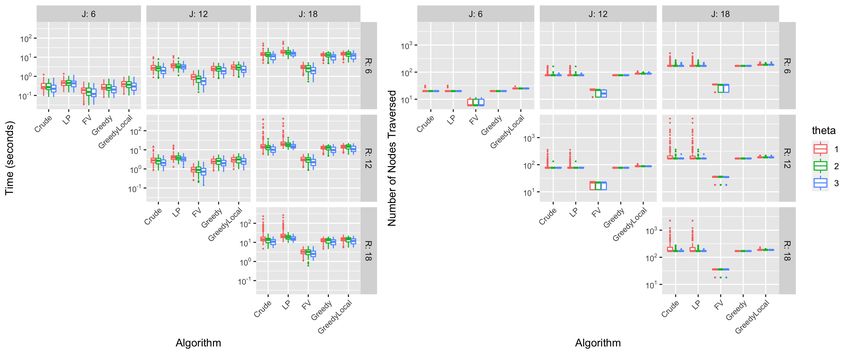
5.1 Speed
There are two useful metrics to consider when evaluating speed in graph search algorithms. The
first is overall time, which we measure in seconds. The second is the number of nodes traversed,
which signifies an efficient algorithm with respect to memory. While time may be a more practically
important metric, if the number of nodes traversed is substantially smaller for a slower algorithm
then potential improvements to memory time or code efficiency may ultimately result in a faster
algorithm. We compare algorithm speed in Figure 3 on the basis of these two metrics.
Figure 3: Speed of algorithms based on time (left) and number of nodes traversed (right)
across different values of J, R, and θ. Results are aggregated over M and I.
Among the exact algorithms, the number of nodes traversed is comparable between both yet
computation time is reasonably higher for LP under most regimes. When exact search is desired,
we recommend the Crude algorithm on the basis of these results. Regarding the approximate algo-
rithms, the FV algorithm is substantially faster than the rest. This difference is by approximately
an order of magnitude in all regimes. The Greedy and Greedy Local algorithms are generally similar
in speed to the Crude exact algorithm, a potentially disappointing result given that Greedy and
Greedy Local operate under no guarantee of providing an exact solution. However, they exhibit
consistent speed results, unlike the exact algorithms which have frequent and extreme high-time
outliers.
Overall, we observe that estimation time generally increases as J increases and decreases as θ
increases. These results should not be surprising: For large J, the algorithms can be slow due to
the massive parameter domain. When θ is small, ranking consensus is weak so search algorithms
15Pearce and Erosheva
may be pulled into many distinct subspaces of the parameter domain. Speed does not change
substantially as R increases.
5.2 Accuracy
We measure accuracy of the approximate search algorithms using two metrics: The first is the
proportion of simulations in which each algorithm returns the true MLE. However, incorrect esti-
mates may be trivially different from the truth, which leads us to our second metric: The Kendall
distance to the true MLE. This measures how far away the estimated ordering of the object quality
parameters are from π̂0 . We compare algorithm accuracy in Figure 4 on the basis of these two
metrics.
Figure 4: Accuracy of algorithms based on the proportion of estimates equal to the true
MLE (left) and Kendall distance to the true MLE (right) across different values
of J, R, and θ. Aggregated over various values of M and I.
The proportion correct will be 1 and the Kendall distance to the true MLE will be 0 for both the
exact algorithms, by definition. For the approximate algorithms, both metrics suggest the order of
least to most accurate approximate algorithm is FV, Greedy, and Greedy Local. We point out that
even though FV was the fastest algorithm, it exhibits the worst accuracy overall, especially when θ is
small. On the other hand, Greedy Local is quite often exactly correct. Accuracy generally improves
in all approximate algorithms as R increases, which makes sense given that partial rankings equate
to less preference information.
In sum, this section has provided insights for practitioners when selecting an estimation algo-
rithm for the Mallows-Binomial model. If exact MLEs are desired, the Crude algorithm is a good
choice. When approximations are satisfactory or required due to computational cost, especially
when J is large or postulated θ is small, we recommend the Greedy Local algorithm due to its high
accuracy or the FV algorithm for a fast and rough approximation of the consensus ranking.
16A Unified Model for Rankings and Scores
6. Analysis of Grant Panel Review Data
We now apply our model to a real data set on grant panel review. After providing an exploratory
analysis, we display and interpret estimation results.
6.1 Exploratory Analysis
We consider one specific instance of grant panel review conducted by the American Institute of
Biological Sciences (AIBS) during Fall 2020, where judges provided both scores and rankings. In
the panel, 9 judges discussed 18 proposals. They were allowed to assign scores between 1.0 and
5.0 in single decimal point increments. After discussion and openly scoring each proposal in turn,
judges were asked to provide top-6 partial rankings. Ties were not allowed. Since judges discussed
every proposal, a proposal not receiving a top-6 ranking was deemed worse than each of the ranked
top-6 proposals. With a few exceptions, all judges scored all proposals and ranked their top 6.
One judge scored only one proposal and did not provide a ranking; another did not provide a
ranking, and a third only provided a top-5 ranking. Based on information from AIBS, missing
data occurred for reasons independent of any characteristics of the proposals, such as child care or
family responsibilities. Thus, it is considered to be missing completely at random and can be safely
ignored during data analysis without biasing estimation results. Figure 5 summarizes the data with
proposal scores on the left and partial rankings on the right.
Figure 5: AIBS grant panel review data. Left: Scores by proposal (boxplots in gray; raw
data in black). Right: Proposals by rank.
We observe a variety of scoring and ranking patterns by proposal. For some proposals all
judges gave identical scores, while for others there was wide disagreement between judges. For
rankings, 13 of the 18 proposals were in at least one judge’s top-6 ranking. However, Figure 5
17Pearce and Erosheva
shows that a smaller subset of proposals were ranked by a majority of the judges (e.g., proposals
1, 7, and 14). Separately, we also measure the consistency of rankings and scores at the judge
level. If the rankings were to always align with the order of the scores, for example, the rankings
may be thought of as providing little additional information. To quantify this, we measure the
Kendall distance (i.e., the number of pairwise disagreements) between each judge’s partial ranking
and the implied order of his/her scores. When a judge does not rank any two proposals, we do
not count potential inconsistencies between them. We found the Kendall distances between each
judges’s partial ranking and score-implied ranking to be {2, 4, 4, 5, 7, 11, 22} (ordered from least to
greatest). Given that each judge only provided a top-6 ranking of the proposals, there is substantial
discordance between rankings and scores at the judge level. We believe this further motivates the
use of a combined model for rankings and scores for this data set.
The AIBS is principally interested in identifying which proposals should receive funding. While
thematic and other considerations also contribute to funding decisions, funding agencies rely on
peer review to identify which proposals are quality proposals and whether proposals can be ordered
or tied in quality. Thus, both estimating proposal quality parameters and identifying a consensus
ranking are of interest. Understanding uncertainty in the estimated consensus ranking is key for
understanding if objects are of similar quality.
We fit a Mallows-Binomial model to the data, in which M = 40, I = 9, J = 18, and R = 6.
In doing so, we make note of a few assumptions. First, we assume that each proposal has a
true underlying quality. The underlying qualities imply a true ordering of the proposals from
best to worst, which we seek to estimate. Second, we assume that the population of judges is
homogeneous in its preferences. This may be interpreted as assuming that all judges use the same
criteria when ranking or scoring and that all variation in scores and rankings is due to random
chance, as opposed to true ideological differences. Third, we assume that all scores and rankings
are conditionally independent given the latent true underlying quality of a proposal and the level
of consensus strength.
6.2 Results
We now present the MLE and the associated bootstrapped 90% confidence intervals of the consensus
scale parameter θ and object quality vector p. Confidence intervals are based on 200 bootstrap
samples. Table 1 contains parameter estimates and Figure 6 displays estimates alongside the data.
In the left panel, expected scores and associated confidence intervals overlay judges’ observed scores.
The right panel is a histogram of the Kendall distance between each judge’s partial ranking and
the estimated MLE of the consensus ranking.
As shown in the left panel of Figure 6, the MLEs of the expected scores approximately equal
the mean observed scores. However, confidence bands reflect information obtained from both scores
and rankings. For example, proposals 8 and 16 have lower confidence limits that are much lower
than the minimum score they received, which is unusual for a measure of the expected (mean)
score. This likely occurs since they were each ranked comparatively better than the scores they
received on average. We also notice that a few proposals share the same MLE of true underlying
quality but are strictly ordered (i.e., not tied) in the consensus ranking. For example, proposals 5
and 9 correspond to p̂5 = p̂9 = 0.563, but proposal 5 is ranked higher than proposal 9 in π̂0 . In this
case, proposal 5 received a marginally worse average score than 9 but was ranked higher. Thus,
the model can capture a difference in ranking while suggesting the true underlying quality is likely
nearly identical. In the right panel, we notice that most judge’s partial ranking mostly aligned
18A Unified Model for Rankings and Scores
Parameter MLE 90% CI Parameter MLE 90% CI
θ 0.529 (0.421,1.124) p10 0.416 (0.308,0.525)
p1 0.272 (0.239,0.306) p11 0.684 (0.642,0.730)
p2 0.683 (0.626,0.729) p12 0.656 (0.565,0.711)
p3 0.666 (0.544,0.766) p13 0.522 (0.481,0.565)
p4 0.575 (0.553,0.616) p14 0.169 (0.150,0.186)
p5 0.563 (0.511,0.646) p15 0.463 (0.374,0.541)
p6 0.400 (0.325,0.453) p16 0.683 (0.646,0.698)
p7 0.153 (0.103,0.199) p17 0.866 (0.850,0.875)
p8 0.750 (0.711,0.750) p18 0.484 (0.444,0.541)
p9 0.563 (0.526,0.588)
π̂0 = {7, 14, 1, 6, 10, 15, 18, 13, 5, 9, 4, 12, 3, 16, 2, 11, 8, 17}
Table 1: Maximum likelihood estimates of model parameters for the AIBS grant panel
review data.
Figure 6: Results overlaid on data. Left panel: Scores by proposal (black) and MLE and
90% confidence intervals of expected score (red). Estimated and true scores are
provided on their original scale. The order of proposals on the x-axis aligns with
the MLE of the consensus ranking in the Mallows-Binomial model. Right panel:
Histogram of Kendall distance dR,J between each judge’s partial ranking and π̂0 .
with the MLE of the consensus ranking. The outlier in the right panel of Figure 6 corresponds to
19Pearce and Erosheva
a judge who assigned top-6 rankings to three proposals with comparatively poor scores (proposals
3, 8, and 16).
We display the estimated consensus ranking and associated 90% ranking confidence intervals
for each proposal based on the Mallows-Binomial model in Figure 7. Additionally, we show results
that would be obtained under two separate ranking aggregation or score aggregation models. The
first model, Converted Scores, uses scoring data and converted ranking data, in which ranking data
is converted into scores for each judge such that the first-ranked object receives that judge’s best
score, the second-ranked object receives that judge’s second-best score, etc., as suggested by Li
et al. (2009). Then, the model uses independent Binomial score distributions for each proposal (no
rankings are modeled). The second comparison model, Converted Rankings, uses ranking data and
converted scoring data, in which each judge’s scores are converted into a ranking by simple ordering
(ties are broken at random). Then, the model uses a Mallows’ distribution to model the ranking
data. Confidence intervals for each model are based on 200 bootstrap samples. (A similar figure
with two additional comparison methods which entirely exclude rankings or scores, respectively, is
provided in Appendix C.)
Figure 7: Estimated ranks and 90% confidence intervals based on scores and partial rank-
ings in Mallows-Binomial (MB ) model, scores and rankings converted into scores
in Binomial models (Converted Scores), or partial rankings and scores converted
into rankings in a Mallows’ model (Converted Rankings). Order of proposals on
x-axis aligns with the MLE of the consensus ranking in the MB model.
We observe in Figure 7 that the Mallows-Binomial model provides a sensible estimated ranking
for each proposal: Each proposal has a unique point estimate for rank place and the associated 90%
20A Unified Model for Rankings and Scores
confidence intervals reflect the scores and ranks it received. For example, proposal 7 was ranked
first by 5 of the 7 judges and had the best average score, but proposal 14 was highly ranked by many
judges and received a similarly high average score. Thus, the 90% confidence intervals of (1,2) for
the rank place of proposals 7 and 14 appear appropriate. On the other hand, proposal 3 received
the 13th best average score, which corresponds to its point estimate for rank place. However, its
90% confidence interval (7,17) for rank place is appropriately wide given its wide range of scores
(minimum 15, maximum 35) and a single fourth-place ranking, which injects uncertainty into the
model. In general, confidence intervals are narrow when consensus between scores and rankings
across judges is strong and wider otherwise.
Results from the Mallows-Binomial model improve upon results from the other models in unique
ways. The Converted Scores model provides similar rank place point estimates to the Mallows-
Binomial model, but with confidence intervals that may be viewed as inappropriate. Converted
scores provide narrow intervals that reflect an artificially inflated sample size (resulting from com-
bining both original and converted scores) but does not account for uncertainty arising from con-
verting ranking data to scores. The Converted Scores model does not estimate the consensus scale
parameter θ.
Point estimates and confidence intervals from the Converted Rankings model differ substantially
from those of the Mallows-Binomial. Differences are particularly apparent for proposals ranked in
7th place or worse, as those proposals generally have less data due to the partial rankings collected.
The model loses precision compared to the Mallows-Binomial model in the top ranking places,
despite having the same number of observations, since scores converted into rankings via ordering
lack information on the strength of the difference in quality between proposals. Furthermore, the
model does not estimate the item quality parameter vector p.
Results from the Mallows-Binomial model allow us to compare proposals with confidence. For
example, the model suggests that proposals 7 and 14 are of similarly high quality, but that relative
quality is harder to differentiate for proposals 1, 6, and 10. These types of comparisons may be
useful when drawing a funding line at the AIBS. If the AIBS can fund, for example, only 6 proposals,
then with 90% confidence they should fund proposals 7, 14, 1, 6 and select two additional proposals
between 10, 15, and 13 (perhaps based on point estimates or a random lottery).
7. Discussion
In this paper, we proposed the first unified statistical model for rankings and scores that does not
involve data conversion, the Mallows-Binomial model. We formulated a computationally efficient
algorithm to find the exact maximum likelihood estimators of model parameters and demonstrated
statistical properties of the model such as bias, consistency, and variance of estimators. This
research aligns well with the recommendations from a peer review study at the 2016 Neural Infor-
mation Processing Systems conference that recommended using both rankings and scores to gain
benefits from each data format (Shah et al., 2018). That study also emphasized the need to design
algorithms to efficiently combine scores and rankings for further guidance on conference submission
quality (Shah et al., 2018, p.27).
In this paper, we applied the Mallows-Binomial model to grant review data which collected both
scores and partial rankings from a panel of judges. The model was used to identify a consensus
ranking based on the scores and partial rankings. The estimated consensus ranking was different
from what would be obtained with comparable models for (converted) scores or rankings alone.
Furthermore, we demonstrated a method to obtain confidence bands of proposal qualities and/or
21Pearce and Erosheva
rank places via the bootstrap that can be used to select proposals that are preferred by reviewers
with statistical confidence. Confidence bands clearly reflect information from both scores and
rankings provided by the judges.
The proposed model is useful whenever both rankings and scores for a collection of objects
are available. Beyond the example presented here, this may occur in a variety of contexts. For
example, relevance of webpages to a search query may be measured from different sources using
either numerical metrics (scores) or ordinal comparisons (rankings). In this example, the object
quality parameters would measure both relative and absolute relevance to the search query, and
the scale parameter would represent consensus among judges. In contrast to methods that convert
rankings and scores into data of a single type, the proposed model removes the potential introduction
of error by using information from both sources directly. Yet, it allows for using both rankings and
scores to express different types of comparison and levels of granularity in preferences. Furthermore,
because both types of data are incorporated in a statistical model, this allows for uncertainty
quantification in the estimation of true underlying quality, consensus, and strength of consensus
when both scores and rankings are present using standard model-based statistical approaches.
Estimation methods presented in this paper for the Mallows-Binomial model can be improved
or extended in a number of ways. Computational efficiency of estimation may be improved via a
different heuristic function in the A* algorithm and permit exact estimation of the model in the
presence of large numbers of objects. Approximate algorithms may be improved to increase ac-
curacy and/or speed. In addition, alternative Bayesian estimation methods may be developed by
extending the work of Vitelli et al. (2018) on the Mallows’ model. Model components may also be
generalized: For example, the Generalized Mallows’ distribution or Infinite Generalized Mallows’
distribution proposed by Meila et al. (2012) may replace the ranking distribution component of our
proposed model. The Plackett-Luce distribution may also replace the ranking distribution com-
ponent, although the downside is that it does not directly include a consensus ranking parameter.
Additionally, the Beta-Binomial distribution may replace the score distribution component in our
proposed model if one was interested in accounting for differences in the variance of object scores
between judges. Lastly, the model may be considered in a latent class framework to identify the
presence of and to measure local consensus among heterogeneous preference groups, e.g., by ex-
tending earlier work on the mixture of Mallow’s distributions (Busse et al., 2007) or Plackett-Luce
distributions (Gormley and Murphy, 2006; Gormley et al., 2009).
22You can also read