ABSTRACT A Brief Introduction to Performing Statistical Analysis in SAS, R & Python - LexJansen
←
→
Page content transcription
If your browser does not render page correctly, please read the page content below
PharmaSUG 2020 - Paper SA-207
 A Brief Introduction to Performing Statistical Analysis in SAS, R & Python
                   Erica L. Goodrich, Brigham & Women’s Hospital, Boston, MA
                  Daniel J. Sturgeon, VA Boston Healthcare System, Boston, MA

ABSTRACT
Statisticians and data scientists may utilize a variety of programs available to them to solve specific
analytical questions at hand. Popular programs include commercial products like SAS® and open source
products including R and Python. This paper aims to present a brief primer into the coding and output
provided within these programs to preform data exploration and commonly used statistical models in a
healthcare or clinical space and looks at the reasons why a user may want to use different programs.

INTRODUCTION
Data science, analysis, and statistics are at a height of use in a variety of industries all over the world.
Depending on your personal or company’s preference you may be more specialized in one software suite
over another. This paper hopes to bring a brief overview on how you may be able to utilize SAS®, R, or
Python for a variety of commonly used statistical analysis.
If you’re comfortable with one of these programs, why bother learning another? There are many different
reasons why this can be useful. Different companies may emphasize use of software due to
infrastructure, previous code that is still used, or due to established leaders within their industries.
Sometimes companies have a focused preference, others allow users to use the software they are most
comfortable using. Knowing more programs can allow for additional employment options.
Outside of a company having a preference, users also may enjoy one environment over another. Some
programs have easier methods for specific data manipulations or statistical methodologies as well. In
some respects, an individual’s abilities to use different programs is like a toolbox; while you may be able
to do the bulk of your work construction work done with a hammer, it may not always be the best tool to
use for the task at hand. Perhaps a job may require use of a screwdriver or a saw to work better! If you
are only comfortable in one software for your job, you may have to work harder rather than smarter on
certain tasks.
Another reason to feel comfortable with different programs is to self-check your results. Coding in more
than one software will give you a double-check on your analysis and output. The more this is done, the
more comfortable you can feel in the additional programs used. This can also lead to new ways of
thinking for problem solving or efficiency!
We aim to discuss data exploration, code and syntax, along with output in SAS®, R, and Python. In
addition, we will raise awareness on why some results may look different between programs and how to
troubleshoot these.

OBTAINING SOFTWARE
SAS® & SAS® UNIVERSITY EDITION
Since you are reading this paper which originates from a SAS® Users Group—we assume that you have
some familiarity with SAS® as a statistical software package. Due to this, we will keep the introduction
short. SAS® is available through SAS® Institute, where more specifics for pricing and availability are
found online at https://www.sas.com/en_us/software/how-to-buy.html. SAS® was initially released in
1976. For those using SAS® software for academic, noncommercial use, SAS® University Edition is

                                                     1
available for free. More information on obtaining SAS® University Edition can be found online at
https://www.sas.com/en_us/software/university-edition.html.

Display 1. Screenshot of the SAS® University Edition website

R & RSTUDIO
The R Project for Statistical Computing is hosted at https://www.r-project.org/. R can be downloaded from
CRAN at the following address: https://cran.r-project.org/mirrors.html. R is an open-source software which
is free to use. An open-source software is a software that can be accessed, used, or modified by
anybody.1 There is no one company which has the sole powers in this case. R was initially released in
1993 and was heavily built upon the previously created S programming language which originated from
1976.2

Display 2. Screenshot of the website for R
In addition to using R, there are Graphic-User-Interfaces available (GUIs) to use with R. One popular R
GUI is RStudio. RStudio is available for free online [https://rstudio.com/products/rstudio/]. The authors of

                                                      2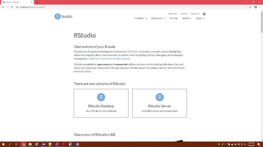
this paper learned R during graduate school and preferred RStudio. Due to this, examples in this paper
will be shown using RStudio’s interface.
Display 3. Screenshot of the RStudio download website
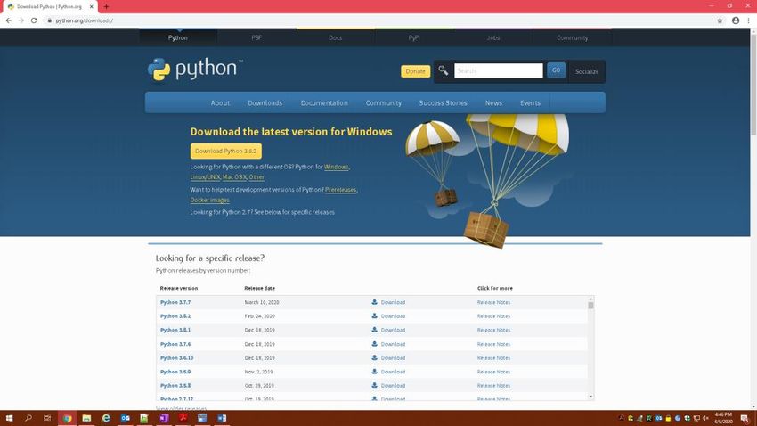
PYTHON & JUPYTER
The third software we are discussing in this paper is another open source computing language called
Python. Python can be downloaded from [https://www.python.org/downloads/]
Figure 4. Screenshot of the Python download website
Like R, Python also has available GUIs. For this paper, examples will be shown using Jupyter notebook
[https://jupyter.org/]. The authors also prefer to use Anaconda for package management and deployment
[https://www.anaconda.com].
3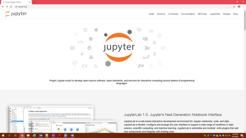
Display 5. Screenshot of the Jupyter download website

INSTALLING NECESSARY SOFTWARE, PACKAGES, AND DATA WRANGLING
Above shows where you can obtain the software of your choice for further use. While SAS® functions
without further installations, R and Python’s open-source nature has additional steps for downloading and
using user-created “packages”. Any user can create a package to provide further use outside of the base
creation of these software. This is sometimes seen in SAS® through created macros, it is not as
commonly done as with R and Python. For statistical analysis examples below, R will need one package
installed. The package needed is called survival, for the survival analysis section. There are many other
packages and methods to accomplish what is shown in this paper as well. Python examples include the
pandas, numpy, os, statsmodels and lifelines packages. New packages come out for R and Python
whenever users and groups decide to create or update them. This paper is trying to show at a minimal a
few methods to get users interested to start and explore what is available for them.
There have been many previous presentations and papers which have shown a nice overview on
downloading, installing, and running data manipulation tasks within different software. For more
information, please see the recommended reading at the end of the paper for more links. Please review
those papers for more detailed instructions.
For this paper, we will explore built in SAS® datasets, found within the SASHELP folder path. They are
accessible to all SAS® users. For sake of examples, these files are converted to .csv file-types, for easier
accessibility in R and Python. Examples will use SASHELP.CARS — 2004 Car Data for most examples,
and SASHELP.BMT — Bone Marrow Transplant Patients for survival analysis examples.5

DATA EXPLORATION
Being able to explore your data, understand the structure, and what variables that are available is pivotal
to meaningful use and analysis. This section will provide an overview on some commonly used methods
between the three programs.

LOOK AT YOUR DATA, A FEW ROWS AT A TIME

                                                     4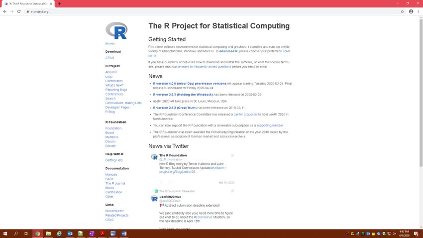
SAS®
PROC PRINT is the quickest way to get output within SAS®. This example shows the first 10
observations in the output window. This is specified by using (obs=10) in the procedure statement.
Without this, all observations will print. From here we can get an overview of what variables are included
and what type of fields data looks like.
proc print data=sashelp.cars (obs=10);
run;

Display 6. SAS® output for displaying header data

R
To look at the data in R can be done by using the head() function. This shows the first 6 observations by
default. Note the number of columns carries over to the lines below due to space available. To specify 10
observations, like SAS®, a command of head(cars, n=10) can be used. The data is the same as
what is shown in SAS®, however in this example there’s an extra column which will be discussed later in
the Logistic Regression analysis below.
head(cars)

Display 7. R output for displaying header data

PYTHON
Much like R, Python will show the first and last five observations for all variables inside of the called upon
dataframe.
print(cars)

                                                      5
Display 7. Python output for displaying header and tail data
METADATA
SAS®
In SAS®, PROC CONTENTS will provide a nice amount of data over the data available in the dataset of
interest. This provides information on the dataset, the number of variables, variable names, type of data
(either character or numerical), and any information on variable length, format, or labeling. In the code
below the extra option of varnum will print the order in the order of the dataset.
proc contents data=sashelp.cars varnum; run;
Display 8. SAS® output for displaying data contents
6R
Getting the names of variables in the dataset of interest can be done by using the names() function. For
more information similar to PROC CONTENTS in SAS®, the str() function can be used. This will provide
information on the dataset structure, the number of observations and variables, the variable type, and the
first few observations.
The output below corresponds to the code:
names(cars)
str(cars)
Display 9. R output for displaying data contents
PYTHON
By leveraging the pandas package, one line of code provides an overview of the dataset of interest. This
provides information of the variables names, counts, data type and missing values information.
cars.info()
Display 10. Python output for displaying data contents
7MEANS, MEDIANS, RANGES, AND OTHER DESCRIPTIVE STATISTICS
SAS®
Specific variables can be called out with a var statement, such as var cylinders; to provide
information only on the cylinders variable. Specific descriptive statistics were called out in the code below.
proc means data=sashelp.cars n mean std min q1 median q3 max maxdec=1;
run;
Display 11. SAS® output for descriptive statistics
R
Descriptive data for continuous variables can be provided using the summary function. If only one
variable was described, it can be called using the dataset name, followed by a dollar sign and the variable
name such as engine size done with the following: summary(cars$EngineSize). R code is case
sensitive, so this needs to be considered with functions, datasets, and variable naming. There are other
packages which can provide different versions of descriptive statistics as well. One example is the Hmisc
package.
summary(cars)
Display 12. R output for descriptive statistics
PYTHON
Using part of the pandas package, one line of code will provide descriptive statistics for all variables
included in the model. This works for categorial and continuous variables.
cars.describe(include = 'all')
8Display 13. Python output for descriptive statistics
FREQUENCIES, CROSS TABS, FOR CATEGORICAL DATA
SAS®
For SAS®, the FREQ procedure can be used to create frequency tables. Both one-way frequencies and
cross-tabulation analysis can be made by specifying one variable or two or more variables separated by
an asterisk. Below shows the count data for one way frequency of the variable ‘Type’.
proc freq data=sashelp.cars;
tables type;
run;
Display 14. SAS® output for one-way frequencies
proc freq data=sashelp.cars;
tables type*cylinders;
run;
9Display 15. SAS® output for cross-tabulation frequencies
R
One-way frequencies and crosstabs can be created in R using the table() function. By listing one or two
variables separated by commas, the frequency data is produced in the format below.
table(cars$Type)
Display 16. R output for one-way frequencies
table(cars$Type,cars$Cylinders)
Display 17. R output for cross-tabulation frequencies
PYTHON
For Python, the pandas package is used. Calling on crosstab (where the pandas package was read in
with the naming convention ‘pd’, the variable of interest is called “Type”, and the columns are specified to
show counts. The example below shows a cross tab, where in place of “count”, the variable of interest is
added.
pd.crosstab(index = cars["Type"], columns = "count")
10Display 18. Python output for one-way frequencies
pd.crosstab(index=cars["Cylinders"], columns=cars["Type"])
Display 19. Python output for cross-tabulation frequencies
STATISTICAL ANALYSIS
Hopefully after exploring the datasets and feeling more comfortable with the data, we will move into
coding needed for some statistical models. Please note that this is more of an emphasis on the coding
needed for the models described below than explaining all output and their related interpretations.
LOGISTIC REGRESSION
SAS®
Using the SASHELP.CARS dataset, a variable is created as a binary indicator for ‘fuel efficiency’. This is
designated if MPG for highway driving is greater or equal than 28 MPG. Where an indicator flag of ‘1’
designates a fuel-efficient vehicle and will be the dependent variable of this model. For running a logistic
regression on fuel efficiency, covariates of horse power, drive train, and weight are considered as
independent variables. Horse power and weight both are continuous variables, whereas drive train is a
categorical variable. In the SAS® code below, drivetrain is added to the class statement, with the ‘Rear’
category being the referent group. Param=ref is an option used for specifying how to handle class
variables. In the model statement, there is an option of (event=’1’). This is used to denote what level to
model the probability for.
data cars;
set sashelp.cars;
11if mpg_highway < 28 then fuel_eff=0;
else fuel_eff=1;
run;
proc logistic data=cars;
class drivetrain(ref="Rear")/param=ref;
model fuel_eff(event='1') = horsepower drivetrain weight;
run;
SAS® provides information on the dataset, the number of observations included, and other information
including model fits information and parameter estimates. SAS® also provides the Odds Ratios by
default. From the results, we see that horsepower, drive train, and weight to be statistically significant
covariates.
12Display 20. SAS® output for Logistic Regression results R Logistic regression model can be run in R by using the glm() function. Within this function, the we are modeling fuel efficiency, following the model covariates with a tilde. Horse power, drive train, and weight are separated by plus signs. In addition, there is a prompt for the dataset and a statement for ‘family’ to specify that this is a binomial distribution. Prior to the model, drive train was converted from a character value to a factor. This was needed for specifying a reference level like what was done in SAS®. If this does not matter, the step can be skipped, and the DriveTrain variable could be added to the model in the place of the relevel() function. From there, the model results are stored into an object called fueleff. The results of the model are presented as output by using the summary() function and then exponentiating the coefficients. The second step uses the exp() function to exponentiate, from the cbind is used to join the character lists together from the parameter estimates and 95% confidence intervals. cars$DriveTrainf
values like the SAS® class statement. In addition, an intercept needs to be manually added to the model.
This is done with the add_constant statement.
import statsmodels.api as sm

x = cars[['Horsepower', 'drivetrain_1','drivetrain_2','Weight']]
x = sm.add_constant(x)
y = cars['fuel_eff']

logit_model=sm.Logit(y,x)
result=logit_model.fit()
print(result.summary2())

Display 23. Python output for Logistic Regression results

KAPLAN-MEIER PLOTS & LOG-RANK TEST
SAS®
Using the SASHELP.BMT dataset, we will explore survival analysis. For this, we have a time variable
marking disease-free progression, called t, a status indicator, which an event time (=1) or a censored time
(=0) and a group variable. The group variable has three levels of and indicates patient risk category. By
default, SAS® creates a KM-curve when using PROC LIFETEST. In addition, test statistics, including
Log-Rank test statistic are included in the output. The model consists of the time variable, and the censor
variable followed by parenthesis to denote which reading is considered for the censored values. We see
from our results, there are statistically significant differences between at least two of the three risk groups.
proc lifetest data=sashelp.bmt;
    time t*status(0);
    strata group;

                                                      14
run; Display 24. SAS® output for Kaplan-Meier curves and Log-Rank statistics R R requires the survival package as one option to run survival analysis methodologies. From there, creating KM curves require a bit more coding than what is provided automatically with SAS®. In this example, the survival model is run within the survfit function. This is saved into an object called bmtdt. This object is then called within the plot function. The plot function has additional options to specify colors and labels. After the plot function, the legend function is used to specify and create the legend of the graph. This specifies labeling, colors, and location of the legend. library(survival) bmtdt
legend("topright",

         c("All", "AML-High Risk", "AML-Low Risk"),

         lty='solid',

         col=c('blue','red','dark green'))

Display 25. R output for Kaplan-Meier curves

From there, to calculate the Log-Rank Test, the survdiff() function is used. This specifies the survival mod
el again and adds in the option rho=0.
survdiff(Surv(T, Status) ~ Group, data=bmt, rho=0)

                     N Observed Expected (O-E)^2/E (O-E)^2/V
Group=ALL           38       24     21.9     0.211     0.289
Group=AML-High Risk 45       34     21.2     7.756    10.529
Group=AML-Low Risk 54        25     40.0     5.604    11.012

 Chisq= 13.8       on 2 degrees of freedom, p= 0.001

PYTHON
Using the lifelines package, the KaplanMeierFitter function is used. First, an object is created called kmf1.
This will be used later to fill in the needed information for drawing the KM curve. A subset of the bmt
dataset is created into three separate groups determined by the risk group status. These are stored in
objects g1, g2, and g3. These then plotted one at a time using the kmf1 object, using the fit function.
These then are called into a graph one group at a time using the plot function as shown below.
kmf1 = KaplanMeierFitter()

                                                     16
g1 = bmt.loc[bmt["Group"] == 'ALL']
g2 = bmt.loc[bmt["Group"] == 'AML-High Risk']
g3 = bmt.loc[bmt["Group"] == 'AML-Low Risk']
kmf1.fit(g1['T'], g1['Status'], label='ALL')
a1 = kmf1.plot(ci_show=False)
kmf1.fit(g2['T'], g2['Status'], label='AML-High Risk')
kmf1.plot(ax=a1, ci_show=False)
kmf1.fit(g3['T'], g3['Status'], label='AML-Low Risk')
kmf1.plot(ax=a1, ci_show=False)
Display 26. Python output for Kaplan-Meier curves
Like R, in Python, the log-rank test is called in a different line of code than the KM curve. The
multivariate_logrank_test function is used for multiple groups, whereas in instances where overall KM
curve was desired, the logrank_test() function itself could be used. The prompts inside are for the time
variable, the groups of interest, and the censor variable of interest. From there, the summary is requested
using the print_summary object.
lrt = multivariate_logrank_test(bmt['T'], bmt['Group'], event_observed =
17bmt['Status'])
lrt.print_summary()
Display 27. Python output for Log-Rank Test
COX PROPORTIONAL HAZARDS EXAMPLE
SAS®
The BMT example can be expanded into using Cox Proportional Hazards models as well. Keeping the
same variables of interest within a PHREG, we can get the Hazard Ratios for group. The coding is similar
to PROC LIFETEST, but rather than treating group as a strata, it is a dependent variable within the
model. Since it is a categorical value, it’s accounted for in the class statement as well.
proc phreg data=sashelp.bmt;
class group(ref='ALL') /param=ref;
model t*status(0)= group/rl;
run;
18Display 28. SAS® output for Cox Proportional Hazards Model R Still using the survival package, to run Cox Proportional Hazards models, the coxph function is used. The inputs are very similar to what is seen in the coding for KM curve and the log-rank test. The model is saved as an object called cphm, and then called using summary() function. cphm
A careful eye will notice that there’s a difference in the results between R and SAS®. There are
differences in coefficient results and p-values. Neither program is wrong- but through practice and
documentation, it can be noted that SAS® and specific R packages may favor different methods as
defaults. In Cox Proportional Hazards models there are different methods for handling tied data which
occurs on the same date. SAS® uses the approximate likelihood of Breslow.[3] R uses the Efron
approximation for ties.[4] If the code is updated to specify method=”breslow” then the output matches
what is seen in SAS®.
cphm
Display 31. Python output for Cox Proportional Hazards Model

CONCLUSION
In short, there are many ways to get the same results depending on the program you choose to use.
There are also minor differences that are in all the three software options which can lead to slightly
different (but not incorrect) output. Being comfortable with different programs allow you to know how
things may differ, be able to work in different environments. In instances where you may need to use one
due to your company’s decisions or your analysis needs you will be able to adapt more quickly.

REFERENCES
1. Open Source Initiative “The Open Source Definition” Accessed April 26, 2020.
https://opensource.org/osd
2. The R Project for Statistical Computing. “What is R” Accessed April 26, 2020. https://www.r-
project.org/about.html
3. SAS® Institute “The PHREG Procedure” Accessed April 27, 2020.
https://documentation.sas.com/?docsetId=statug&docsetTarget=statug_phreg_toc.htm&docsetVersion=1
5.1&locale=en
4. The R Project for Statistical Computing. “Package ‘survival’” Accessed April 27, 2020. https://cran.r-
project.org/web/packages/survival/survival.pdf
5. SAS® Institute “SASHELP datasets information” Accessed April 21,2020.
https://support.sas.com/documentation/tools/sashelpug.pdf

RECOMMENDED LINKS
•   SAS® Institute "How to Buy" https://www.sas.com/en_us/software/how-to-buy.html
•   SAS® Institute “SAS University Edition” https://www.sas.com/en_us/software/university-edition.html
•   R https://www.r-project.org/
•   RStudio https://rstudio.com/

                                                     21
• Python https://www.python.org/
• Jupyter https://jupyter.org/
• Anaconda https://www.anaconda.com/
RECOMMENDED READING
• Bretheim DR. 2019. "Comparing SAS® and Python – A Coder’s Perspective"
https://www.sas.com/content/dam/SAS/support/en/sas-global-forum-proceedings/2019/3884-2019.pdf
• Bulaienko 2016. "SAS® and R - stop choosing, start combining and get benefits!"
https://www.lexjansen.com/pharmasug/2016/QT/PharmaSUG-2016-QT14.pdf
• Duraisamy S. 2018. "A Gentle Introduction to R From A SAS Programmer's Perspective"
https://www.lexjansen.com/pharmasug/2018/HT/PharmaSUG-2018-HT04.pdf
• Forman C. 2018. “SAS® and Python: The Perfect Partners in Crime”
https://www.sas.com/content/dam/SAS/support/en/sas-global-forum-proceedings/2018/2597-2018.pdf
• Li JJ. 2019. "Python and R made easy for the SAS® Programmer"
https://www.lexjansen.com/wuss/2019/183_Final_Paper_PDF.pdf
• Lee K. 2019. “Why we should learn Python”
https://www.pharmasug.org/proceedings/2019/AD/PharmaSUG-2019-AD-136.pdf
• Luebbert J, Myneni R. 2019 "SAS® and Open Source: Two Integrated Worlds"
https://www.sas.com/content/dam/SAS/support/en/sas-global-forum-proceedings/2019/3415-2019.pdf
• Korchak 2018. "Expand Your Skills from SAS® to R with No Complications"
https://www.lexjansen.com/pharmasug/2018/BB/PharmaSUG-2018-BB22.pdf
• Takanami Y. 2019. “Interaction between SAS® and Python for Data Handling and Visualization”
https://www.sas.com/content/dam/SAS/support/en/sas-global-forum-proceedings/2019/3260-2019.pdf
• Molter M. 2019. "Python-izing the SAS Programmer"
https://www.lexjansen.com/pharmasug/2019/AP/PharmaSUG-2019-AP-212.pdf
CONTACT INFORMATION
Your comments and questions are valued and encouraged. Contact the author at:
Erica Goodrich
Brigham and Women’s Hospital
TIMI Study Group
60 Fenwood Road, Suite 7022
Boston, MA 02115
egoodrich@bwh.harvard.edu
617-278-0316
Any brand and product names are trademarks of their respective companies.
22You can also read


