ABSTRACT Enabling SAS Forecast Server To Perform Best On Automated walmart.com Sales Forecasting

Paper 3740-2019

 Enabling SAS® Forecast Server To Perform Best On Automated
                walmart.com Sales Forecasting
                 Alexander Chobanyan, Sangita Fatnani, Walmart Labs

ABSTRACT

Generating sales forecast for online retailer the size of Walmart.com is a big and complex
task. Our online sales are of massive magnitude every day. Our sales pattern for Holiday
season between Thanksgiving and Christmas is very different from the rest of a year. In
addition, sales patterns significantly shift between different lines of goods distribution (such
as shipping directly to customer’s home vs. shipping to store for customer’s pick-up) as well
as between different departments (such as Electronics sales vs. Pharmacy sales). Our daily
Statistical Forecast helps the business to with long-term financial planning as well as with
evaluating efficiency of particular promotion, which can run just for one day or so.

SAS® Forecast Server provides a great infrastructure to automatically diagnose each of
hundreds of Sales time-series at various levels of sales and time hierarchies and find the
best time-series model for each of these time-series. However, traditional time-series
modeling with SAS Forecast Server assumes specifying just one periodicity value for data.
Our data are “highly twice periodic” with “first” periodicity being weekly periodicity of daily
lag 7 and “second” periodicity being “yearly” periodicity of varying lag of 365-366 days.

In addition, Thanksgiving Holiday seasons for adjacent years are separated by uneven
number of days, and many departments have sales that are subject to multiplicative
seasonality for holidays and additive seasonality for the rest of the year thus making it hard
for any classical time-series model to forecast well for both season and off-season periods.

In this paper we go through data decomposition / re-assembly steps which address
mentioned challenges, significantly improve SAS® Forecast Server performance on our data
and allowing us to achieve daily site-total forecasting accuracies in upper 90s

INTRODUCTION
Generating accurate sales forecasts for major on-line retailer the size of Walmart.com is not
a straightforward task. Sales patterns significantly differ between different Distribution
Channels such as “Shipping to Customer’s Home”, “Picking Up from Walmart store” and
others. Also patterns differ between different departments. For example, departments such
as “Electronics” show complex sales patterns with additive growth through most of the year
except “Holiday Season” that starts from late October and ends with Christmas sales.
“Holiday Season” daily sales of “Electronics”-like departments may exceed by order the
regular daily sales for the rest of the year. In addition, behavior of just “Holiday” promotion-
driven part of sales is more likely to show multiplicative growth year over year. In contrast
to “Electronics”, “Pharmacy” sales pattern is much less sensitive to “Holiday Season” part of
the year, as, naturally, our demand for drugs/medicine is much less sensitive to holidays
and keeps stable behavior pattern throughout whole year.
In addition, catching sales patterns at daily level of granularity has it’s own challenges.
Online sales patterns have both, weekly and yearly seasonality, which make it difficult to
describe them with classical time-series approaches such as Exponential Smoothing or
ARIMA(X) which assume just single seasonality lag.

                                               1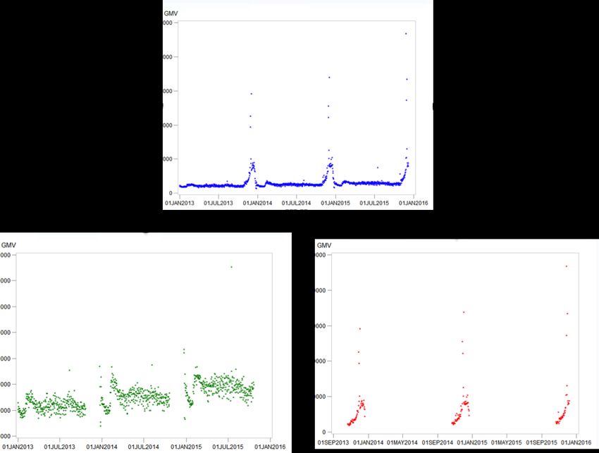

Finally, big sales days such as Black Friday and Cyber Monday and sales patterns, which
surround these days are not evenly separated in time from year to year which adds
additional challenge to consider properly for good forecasting solution.
Using SAS® Forecast Server (SAS® FS) APIs such as proc HPFDiagnose and HPFEngine [2]
helps to address at scale many challenges related to diversity of sales patterns among
different Distribution Channels, Departments, Categories, Sub-Categories, etc. Forecast
Server’s primary advantage over its peers is the ability to specify time-series model search-
space and search performance criteria for a given data segment in contrast to the need of
specifying particular model (with even automatically found model parameters). However,
challenges related to mixed additive and multiplicative seasonality patterns, simultaneous
weekly and yearly periodicities still remained our opportunities to address.
In this paper we describe data pre/post processing steps that help Forecast Server to
significantly increase it’s performance on walmart.com sales data, while keeping the solution
simple and scalable. In particular, we show how “Off Holiday season” sales can be
normalized with respect to day of a week to reduce seasonality to remain calendar year-
based only.
Also, we demonstrate our approach of data decomposition into “regular baseline sales”
series and “holiday” promo sales which allow SAS® Forecast Server’s model search
algorithm to converge to additive seasonal model for “regular” sales and multiplicative
seasonal model for “holiday” sales. We also show how to “center” holiday sales data around
Black Friday / Cyber Monday big sales days, so that holiday sales weeks of adjacent years
are nicely separated by same (multiple of seven) number of days before we feed “Holiday”
data into Forecast Server’s search engine. After we use SAS® Forecast Server to generate
predictions for both “Holiday” and “baseline” parts of data, we show how to apply weekly
profile back to “baseline” forecast and reassemble final forecast by merging “baseline” and
“holiday” outputs together.
Overall, our data decomposition/reassembly approach generated stable forecasts, which
increased both daily and monthly MAPE forecast accuracies by couple of percentage points
reaching upper 90%s for monthly Lag 1 accuracies throughout 2016-2018 years.

BACKGROUND
Our goal was to design scalable, configurable, accurate and simple sales forecast solution
for our Finance team. The requirement was to provide weekly updates for forecast in daily
and monthly time-buckets. Forecast had to be provided at several aggregation levels of
sales hierarchy including “Grand Total” Level, “Distribution Chanel” level (which separated,
for example, items shipped to customer’s home vs items picked up from store vs items sold
on our Marketplace platform by third-party Merchants), and other lower levels including
Super Department, Department, Category and Sub Category. Forecast Monthly Lag 1
accuracy and Daily Lag 1 – Lag 7 accuracies were diligently tracked and compared against
“reference” financial plan in the frames of Forecast Value Add [1] Methodology. (Here, “Lag
n” Forecast is defined as the forecast for the nth time-period in a forecasting horizon.)
Overall, our forecasting hierarchy includes couple of hundreds of time-series/forecasts with
very diverse data patterns. In addition, behavior of our sales for big subset of
Departments/Distribution channels significantly differs during so called “Holiday Season”
with respect to the rest of the year. We define as “Holiday” the time-period, which usually
starts late October and ends with Christmas holiday.
We follow classical forecasting system architecture / processing steps that include acquiring
initial dataset of transactions, segmenting them into parts controlled by the same
aggregation bucket and same SAS forecast Server’s treatment, aggregate transactions, do

                                             2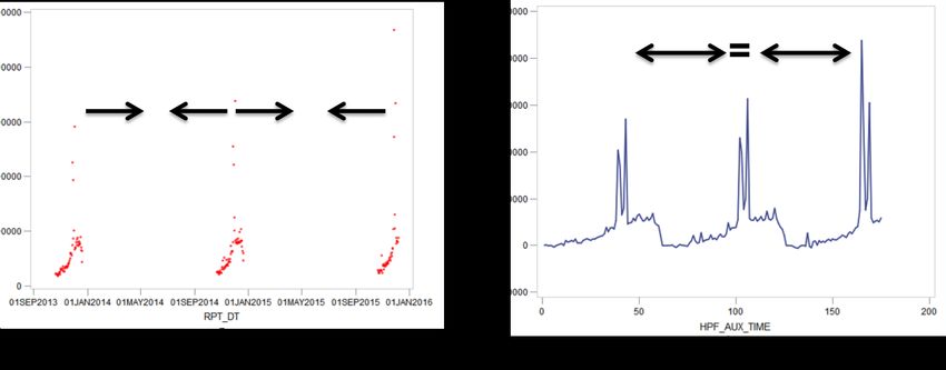

aggregated data pre-processing, generate forecasts for each aggregated segment, apply
data post-processing, perform forecast reconciliation / aggregation to reporting level and
then pass it to downstream system. This work is dedicated to describing our data pre and
post processing methodologies.

Figure 1. Diagram of Forecast Process Architecture. This work describes Pre- and
Post- processing steps to ensure better accuracy of SAS Forecast Server
Before we go to our pre and post processing challenges, let us first state that actual
forecasting part of our solution is built on SAS® Forecast Server APIs (primarily procs
HPFENgine and HPFDiagnose [2]). In our opinion, unique advantage of using SAS® Forecast
Server is it’s ability to quickly automatically converge for each given time-series to best-
suited model family and then to a particular model.
Reference open source solutions would rather require a particular model (such as ARIMA
with given p,d and q or specific model from ESM family) to be defined for each given
forecasting segment.
In contrast, with SAS Forecast server, we define for each segment rather group of family
models (such as for example all ARIMA models with some upper restrictions on p,d and q
parameters and whole ESM family), enable/disable automated attempt to apply EXP, LOG or
BOX-COX transformation, configure model search space with restrictions imposed by our
data segment-specific knowledge, configure conditions of the competition (such as portion
of holdout data, error measure to minimize, etc.) and let SAS® Forecast Server to do the
rest.
For each given time-series from a data segment, SAS® Forecast Server examines the data,
converges first to the best family model and then to the best model with optimized
parameters.
Thus usage of SAS® Forecast Server’s intelligent model search engine helped to make our
data segments more generic while reducing their number and still addressing diversity of
our sales data patterns.
However, we still had to address number of opportunities with enabling Forecast Server to
perform even better.

                                             3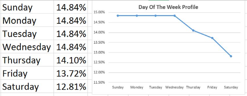

First, Forecast Server configuration allows specifying just one parameter of seasonality.
However, our need to be accurate in daily buckets dictated a need to operate with daily
time-series, which were highly “double-periodic”: natural year-based seasonality (daily lag
365-366) with big sale spikes within months of November-December and also weekly
seasonality (daily lag 7). We figured out, for example, that for some high-volume segments
our customers do significantly less shopping on Saturdays while doing more on Mondays.
Not treating either of these periodicities adequately has immediate impact in daily forecast
accuracy.
Second, our sales growth pattern during “Holiday Season” for many segments is a
composite of additive growth of baseline sales, which happens coherently with sales growth
for the rest of the year and promotional sales, which are more subject to multiplicative
growth. Thus there is an imminent need to model “regular” component of sales time-series
with additive models (such as, for example, Winters Additive Seasonal Smoothing, where
trend is modeled as an additive factor) and model “promotional” component with
multiplicative models where year over year trend is modeled rather as a multiplicative
factor. In addition, impact of sales price discounts has to be modeled differently during
“Holiday” and “Off-Holiday” periods, as sales are much more sensitive to price changes
during “Holiday” times.
In next sections we will talk about how we address “double-periodicity” opportunity of our
data and also about how we do decomposition and reassembly of data into “regular” and
“promotional” components to achieve better prediction accuracy.

“NORMALIZING” DAYS OF A WEEK
In this section we talk about our methodology to pre-process “off-holiday” period sales
which “re-shuffles” sales volume between days within the same week while “removing”
weekly seasonality feature from data. At the same time we store this “weekly” seasonality
aside as “day-of-a-week” profile which we apply back to “off-holiday” daily forecast once it
is generated.
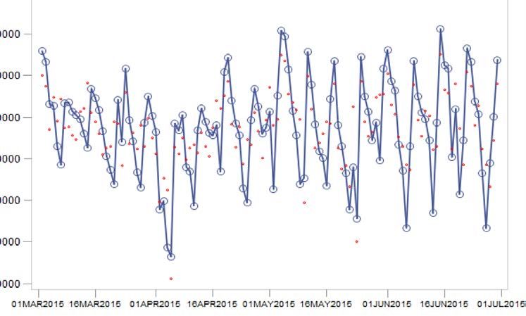
Figure 3 shows regular daily sales pattern of one of our large sales segments during regular
“off-holiday” months of 2015. One can clearly see highly–revealed weekly periodicity (blue
line) with minimal sales occurring on Saturdays.
One naïve periodicity-removal approach can be as simple as splitting each sales time-series
into seven isolated time sequences: one for for all Mondays, second for all Tuesdays, etc.
This approach, however, would decrease amount of data for subsequent time-series model
fitting by a factor of seven thus not allowing to consider more complex time-series models
for future modeling and making whole seven sub-sequences more vulnerable to over-fitting.
Another considered approach is to use SAS® Forecast Server’s option to specify exogenous
variables and code-in days of a week with dummy variables. However, in current
implementation of Forecast Server, consideration of exogenous variables via SAS® Forecast
Server configuration option would essentially limit scope of family models to only ARIMA(X),
or at least would put ARIMA(X) family in much preferable position when competing with
other family models for accuracy.
When selecting our approach we were primarily motivated by accuracy win and also by
principle of statistical simplicity that suggests choosing the simplest approach among
similarly performing ones.
Finally, we converged to the following straightforward solution to reduce day of a week
driven seasonality, while trying to do our best for not over-fitting the data.

                                             4

First, we conduct statistical test to ensure if we have enough data-driven evidence that
particular day of a week has sales significantly higher/lower from it’s peers.
We consider last 30 weeks of regular sales, while computing for iteration 1 the mean and
standard deviation of a mean of all Monday sales, Tuesday sales, etc. Thus we obtain seven
mean numbers and seven standard deviations of a mean (of seven respective days of a
week). For each day of a week we also obtain “reference” average sales volume across all
other days of a week together with it’s standard deviation.
Then we test each of seven day-of-a-week sample mean daily sales for having evidence to
be different from their respective “reference” values. In other words, our null hypothesis H0
here is assumption that sales falling on tested day of a week are equal to 1/7th sales volume
of a week. Note, that we make sure that we exclude all weeks with special sales, such as,
for example, Easter week, from our data sample of recent 30 weeks.
We assume normality for our day-of-a-week specific sample means and use t-test to see of
we have enough evidence to reject H0 with significance level 0.05. Out of all day-of-a-week
candidates with p-values smaller than 0.05 we select day-of-a-week with the lowest p-
value.
Then, for the next iteration we put sales of a “winner” day-of-a-week aside. Now we have
six days of a week data remaining with null hypothesis H0 now being that each of remaining
six days of a week carry 1/6th of volume of these six days combined.
We continue with next iterations until we either select all days of a week or unless at certain
point there are no more “winners” (i.e. we are not able anymore to reject H0 at 0.05
significance level).

Figure 2. Example of day of a week profile with Thursday, Friday and Saturday
only showing significant distinction in sales compared to other days of a week
As a next step we record “day-of-a-week profile” which consists out of seven proportion
values. Proportion for each selected day (with obtained evidence of “behaving” different
from it’s peer days) will be total sales amount for that day over last 30 weeks divided by
overall 30-week sales amount. All remaining days of a week that did not get enough
evidence to reject H0 will get equal proportion. Figure 2 shows example of day of a week
profile with Saturday, Friday and Thursday only showing significant sales deviation pattern
from the rest of days.
The last step normalizes daily history by reshuffling some of daily volume between days of
the same week guided by day-of-a-week profile proportions. Variability of daily history thus
gets significantly reduced, while weekly seasonality gets separated out of data and
essentially stored in day-of-a-week profile. Figure 3 shows original weekly-seasonal series

                                              5

shown as blue line, while adjusted by day-of-a-week profile series is shown as red dots. One
can clearly see reduced data variability for “red dot” series with respect to the one shown by
blue line.

Figure 3. Original daily sales with weekly periodicity (blue line) and adjusted
series (red dots) showing significantly reduced variability
Adjusted time-series then is ready to be passed to SAS® Forecast Server APIs with just one
yearly periodicity specified. Once “off holiday” forecast is generated for adjusted series, we
need to put weekly seasonal pattern back in. We do it by applying “in-reverse” our day-of-
a-week profile to the forecast. Both, transformations of the history and then forecast are of
the similar nature. The only difference between history and forecast transformation is as
follows: for history transformation we move volume from days of a week with consistently
bigger sales to those with consistently smaller sales thus “flattening” daily history. And for
the forecast we put weekly “curls” back in by moving forecast volume from days with
consistently lower sales to days with consistently higher sales.
Let us note that transformations of both weekly-seasonal history and then forecast happen
without moving, increasing or decreasing of weekly volume of either history or forecast. It is
all about just re-shuffling weekly sales volume between days of a week, while first
“removing” weekly periodicity from data, recording it in day-of-a-week profile and then
reapplying it back to the forecast by reshuffling forecast volume between days of the same
week.

“REGULAR”/”PROMO” COMPONENTS DECOMPOSITION & FORECAST
In this section we show our work on decomposition of walmart.com time-series data into
“regular” or “off-season” and “holiday season” parts to enable Forecast Server to converge
to the best model for each of components. Then we show how to re-assemble component
forecasts back to the final sales forecast.
Overall, we address the challenge of different behavior pattern of our regular baseline sales
and our holiday promotional sales. Moreover, for many of our segments, our “holiday sales”
(starting from end of October and ending with Christmas sales) can be viewed as
superposition of “every day” sales and promotional part highly sensitive to price changes &
marketing campaigns.

                                              6

We emphasize that following the principle of statistical simplicity, we bring in external
variables such as initial markup unit (IMU%) or marketing dollars only if event does not
repeat or repeats in very different ways year over year and thus cannot be handled by
seasonal time-series model. Decomposing sales time-series into promo and non-promo
parts brings an important advantage of considering different set of exogenous variables for
each of the components.
First step in decomposition is to initialize “baseline” time-series as time-series with weekly-
adjusted values as defined in previous section and missing values for “holiday” periods of all
years considered in the sales history (See Fig 4., lower left component). It is important to
ensure that each year has defined “holiday” season consisting out of multiples of seven days
and each year’s “holiday” period has the same number of days prior to and past
Thanksgiving day.

Figure 4. Split original time series into baseline and promotional parts
Second step is to feed “baseline” series with missing values to SAS® Forecast Server and
have Forecast Server to generate not only forecast to future time horizon, but also do ex-
post “baseline” forecast into “Holiday” periods initialized as missing. Thus, for baseline
forecast falling into “holiday” periods we are likely to get “spike-free” “placeholders”. At
later steps, on top of these “placeholders” we add promotional forecast generated
separately.
Third step is to take “holiday”-period related portion of original time-series (without
performing any day-of-a-week periodicity removal) and subtract from each sales value it’s

                                              7

respective baseline prediction obtained at Second step. Thus we get promotional-driven
component only.
Fourth step is to “align” promotion data-periods for different years next to each other while
introducing artificial time-scale. If, for example, ”holiday” period consists out of 63 daily
observations (keep in mind that we want our “artificial” promo year to remain multiple of
seven), and we have three years in our history then “promo” time-series will have 189 data
points. Within new time-scale last day of previous year promo period will be directly
followed by the first day of “promo” period of next year (see Fig 5).

Figure 5. Converting of promotional time-series into “artificial” time-scale where
Thanksgiving spikes are evenly spaced.
If all previous steps are done right then each Thanksgiving day and all big sales days that
surround Thanksgiving for a given year will be separated from their previous year’s peers by
same, multiple of seven number of days.
Fifth step is to feed “holiday” data into SAS® Forecast Server’s search engine. We will need
to specify right seasonality lag parameter (length of “holiday” period). Note, that under
given setup SAS® Forecast Server is positioned to perform better: Our “holiday” periods are
aligned to each either, are designed to have exact number of days separating one year from
the following year. Plus each period is designed to contain number of days as multiple of
seven which allows to better capture weekly fluctuations without application of day-of-a-
week adjustments to “holiday” period data.
At Sixth step we diligently map future “holiday” period promo forecast days from artificial
time-scale to their original calendar time-scale. Then we add promo forecast values to their
respective baseline “placeholder” forecast values obtained at Second step.
Finally, we re-apply day-of-a-week fluctuations for “off-holiday” period to “adjusted” “off-
holiday” forecast as described in previous section.

RESULTS & CONCLUSION
We successfully reduced (in data) and re-instated (in forecast) day-of-a-week based
periodicity and applied our data decomposition and reassembly technique to walmart.com
big segments to achieve better performance with SAS® Forecast Server driven Sales
forecast throughout years 2016-2018 (inclusive).
Our decomposition technique allows SAS Forecast Server’s search engine to converge to
additive seasonal model for “baseline” part of sales and to multiplicative seasonal model for

                                             8

“promotional” part. Also decomposition brings flexibility to consider different set of
exogenous variables for “Promotional” part while leaving “baseline” part as simple as
possible which helped to avoid over-fitting and eventually achieve better performance
results.
Our MAPE Site total daily error got reduced from 10% to 5% as a direct consequence of
application of techniques described in this work. Monthly site total Lag 1 MAPE error was
reduced to 2%.

REFERENCES
[1] Gililand, Michael. 2010. The Business Forecasting Deal. New York: John Wiley & Sons.
[2] SAS Institute Inc. 2009. SAS®. HighPerformance Forecasting 3.1: User’s Guide. Cary,
NC: SAS Institute Inc.

ACKNOWLEDGMENTS
We would like to acknowledge Jaya Kolhatkar and Lin Ye for their continuous feedbacks and
support throughout 2015-2018, which helped a lot to deliver results.

CONTACT INFORMATION
Your comments and questions are valued and encouraged. Contact the author at:
    
                                            9