Aerosol type classification analysis using EARLINET multiwavelength and depolarization lidar observations
←
→
Page content transcription
If your browser does not render page correctly, please read the page content below
Atmos. Chem. Phys., 21, 2211–2227, 2021
https://doi.org/10.5194/acp-21-2211-2021
© Author(s) 2021. This work is distributed under
the Creative Commons Attribution 4.0 License.

Aerosol type classification analysis using EARLINET
multiwavelength and depolarization lidar observations
Maria Mylonaki1 , Elina Giannakaki2,3 , Alexandros Papayannis1 , Christina-Anna Papanikolaou1 , Mika Komppula3 ,
Doina Nicolae4 , Nikolaos Papagiannopoulos5,6 , Aldo Amodeo5 , Holger Baars7 , and Ourania Soupiona1
1 Laser Remote Sensing Unit, Department of Physics, National and Technical University of Athens, Zografou, 15780, Greece
2 Department   of Environmental Physics and Meteorology, Faculty of Physics, National and Kapodistrian University of Athens,
Athens, Greece
3 Finnish Meteorological Institute, P.O. Box 1627, 70211 Kuopio, Finland
4 National Institute of R&D for Optoelectronics (INOE), Magurele, Romania
5 Consiglio Nazionale delle Ricerche, Istituto di Metodologie per l’Analisi Ambientale (CNR-IMAA),

C.da S. Loja, Tito Scalo (PZ), 85050, Italy
6 CommSensLab, Dept. of Signal Theory and Communications, Universitat Politècnica de Catalunya, Barcelona, Spain
7 Leibniz Institute for Tropospheric Research, Leipzig, Germany

Correspondence: Maria Mylonaki (mylonaki.mari@gmail.com)

Received: 18 August 2020 – Discussion started: 27 October 2020
Revised: 26 December 2020 – Accepted: 4 January 2021 – Published: 15 February 2021

Abstract. We introduce an automated aerosol type classifica-        nally, our results show that NATALI has a lower percentage
tion method, called Source Classification Analysis (SCAN).          of unclassified layers (4 %), while MD has a higher percent-
SCAN is based on predefined and characterized aerosol               age of unclassified layers (50 %) and a lower percentage of
source regions, the time that the air parcel spends above           cases classified as aerosol mixtures (5 %).
each geographical region, and a number of additional cri-
teria. The output of SCAN is compared with two indepen-
dent aerosol classification methods, which use the intensive
optical parameters from lidar data: (1) the Mahalanobis dis-        1   Introduction
tance automatic aerosol type classification (MD) and (2) a
neural network aerosol typing algorithm (NATALI). In this           Aerosol particles directly affect the Earth’s radiation budget
paper, data from the European Aerosol Research Lidar Net-           by interacting mainly with solar radiation through absorption
work (EARLINET) have been used. A total of 97 free tro-             and scattering (aerosol–radiation interaction – ARI) (Hobbs,
pospheric aerosol layers from four typical EARLINET sta-            1993). Furthermore, aerosols affect cloud formation and be-
tions (i.e., Bucharest, Kuopio, Leipzig, and Potenza) in the        havior, not only serving as seeds (cloud condensation nuclei,
period 2014–2018 were classified based on a 3β + 2α + 1δ            ice nuclei) upon which cloud droplets and ice crystals form,
lidar configuration. We found that SCAN, as a method inde-          but also influencing the cloud albedo due to changing con-
pendent of optical properties, is not affected by overlapping       centrations of cloud condensation and ice nuclei, also known
optical values of different aerosol types. Furthermore, SCAN        as the Twomey effect (Twomey, 1959; Boucher et al., 2013;
has no limitations concerning its ability to classify different     Rosenfeld et al., 2014, 2016).
aerosol mixtures. Additionally, it is a valuable tool to classify      The light detection and ranging (lidar) technique, which is
aerosol layers based on even single (elastic) lidar signals in      based on the active remote sensing of the atmosphere (Weit-
the case of lidar stations that cannot provide a full data set      camp et al., 2005), has received quite a lot of attention be-
(3β + 2α + 1δ) of aerosol optical properties; therefore, it can     cause of the multiple possibilities to retrieve near-real-time
work independently of the capabilities of a lidar system. Fi-       information on the vertical structure and the composition of
                                                                    the atmosphere with high spatial (i.e., down to a few meters)

Published by Copernicus Publications on behalf of the European Geosciences Union.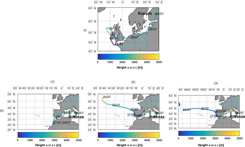
2212                                                                    M. Mylonaki et al.: Aerosol type classification analysis

and temporal (i.e., down to seconds depending on the system)        the aerosol intensive optical properties as stated previously
resolution. Specifically, multiwavelength Raman and depo-           (Nicolae et al., 2018b; Voudouri et al., 2019), a more generic
larization lidars can be used for aerosol detection and char-       aerosol classification code free from these defects is needed.
acterization (i.e., dust, smoke, continental). They can provide        Therefore, in this work, we develop an improved au-
vertically resolved information on extensive and intensive          tomated layer classification algorithm based on air-mass
aerosol optical properties (Freudenthaler et al., 2009; Nico-       backward-trajectory analysis and satellite data. The algo-
lae et al., 2006; Burton et al., 2012; Groß et al., 2013; Gi-       rithm, called Source Classification Analysis (SCAN), is
annakaki et al., 2016; Soupiona et al., 2018, 2019). These          based on the amount of time that the air parcel spends above
properties are the particle backscatter (bλα ) and extinction       an already characterized aerosol source region and a num-
coefficients (eλα ), the lidar ratio (LRλα ), the Ångström ex-      ber of additional criteria. This algorithm, being independent
ponent extinction (Aeλα/λβ ) and backscatter (Abλα/λβ ), and        of aerosol optical properties, provides the advantage that its
the particle linear depolarization ratio (PLDR). Towards this       classification process is not affected by overlapping values
direction, the large majority of European Aerosol Research          of optical properties representing more than one aerosol type
Lidar Network (EARLINET) stations use multiwavelength               (e.g., clean continental, continental polluted, smoke). Fur-
Raman lidar systems that combine detection channels at both         thermore, it has no limitations concerning its ability to clas-
elastic and Raman-shifted signals and are equipped with de-         sify aerosol mixtures. Finally, it can be useful for all types
polarization channels (Pappalardo et al., 2014).                    of lidar systems (independently of the number of channels
   Until recently, the identification of aerosol layers was         used) and for other network-based systems (radar profilers,
based, apart from aerosol lidar data, on air-mass back-             sun photometers).
trajectory analysis, atmospheric models (e.g., DREAM;                  In this paper, we use SCAN, MD, and NATALI as classi-
Basart et al., 2012), concurrent satellite products (MODIS          fiers to assign lidar observations to the pre-specified aerosol
dust and fire data; e.g., Giglio et al., 2013), and ground-based    classes. The three different aerosol classification methods are
photometric data (Papayannis et al., 2005, 2008). It is well-       described in Sect. 2, while Sect. 3 provides a discussion of
established that air-mass trajectory analysis (back to several      the results and a comparison between them. Finally, Sect. 4
hours) with the HYSPLIT (Draxler et al., 2013) or FLEX-             provides the conclusions of our study.
PART (FLEXible PARTicle dispersion model; Stohl et al.,
2005) models ending above the observation station is used
in order to identify the air-mass origin of the detected layer.     2     Methodology
However, this case-by-case aerosol layer identification is nei-
ther objective nor automated.                                       2.1     Aerosol layer classification algorithms
   To overcome this defect, two automated methods have
been developed recently to classify aerosol layers observed         2.1.1    Neural network aerosol classification algorithm
by lidars: (1) the Mahalanobis distance aerosol classifi-
cation algorithm (MD) (Papagiannopoulos et al., 2018),              NATALI (Nicolae et al., 2018a) is an automated, optical-
which uses lidar intensive properties (LRλα , the lidar ratio       property-dependent aerosol layer classification algorithm.
– LRλ1 / LRλ2 , Aeλα/λβ , Abλα/λβ , and PLDR if provided) in        The typical aerosol profiles (3bλα + 2eλα + PLDR, optional;
order to classify the measured aerosol layers into a number         in NetCDF format) from the EARLINET database are used
of aerosol types, and (2) a neural network aerosol classifi-        as inputs in order to retrieve the mean aerosol optical prop-
cation algorithm (NATALI) (Nicolae et al., 2018a), which is         erties within the layer boundaries indicated by the gradient
based on artificial neural networks (ANNs) trained to esti-         method (Belegante et al., 2014). The learning process of the
mate the most probable aerosol type solely from a set of mul-       ANN has been performed using a synthetic database devel-
tispectral lidar data (color index – CI, color ratio – CR, LRλα ,   oped by Koepke et al. (1997) along with the T-matrix numer-
Aeλα/λβ , Abλα/λβ , and PLDR if provided). In reality, inten-       ical method (Waterman, 1971; Mishchenko et al., 1996) to it-
sive aerosol optical properties can vary greatly even for sin-      eratively compute the intensive optical properties of six pure
gle aerosol types. For example, Nicolae et al. (2013) showed        aerosol types (the first six aerosol types in Table 1) presented
that fresh biomass burning aerosols have higher Ångström            to the artificial neural networks to perform the typing. The
exponents and refractive indexes than aged ones. Addition-          synthetic database is built for 350, 550, and 1000 nm wave-
ally, according to Veselovkii et al. (2020), the lidar ratio val-   lengths, which are then rescaled to the usual lidar wave-
ues of dust aerosols can vary greatly depending on the source       lengths (i.e., 355, 532, and 1064 nm) using an Ångström ex-
region mineralogy. Thus, the physicochemical modifications          ponent equal to 1. The mixtures are obtained through a lin-
the aerosols undergo, from the time they are created to when        ear combination of pure aerosol properties (Nicolae et al.,
they are finally observed, change their geometrical, size, and      2018a).
optical characteristics. As a result, their optical properties         Two classification schemes are used with different aerosol
change as well. Taking into account that both NATALI and            type (classification) resolutions when particle depolarization
MD experience several limitations, as they request as input         data are available. The first one is applied when all the high-

Atmos. Chem. Phys., 21, 2211–2227, 2021                                               https://doi.org/10.5194/acp-21-2211-2021
M. Mylonaki et al.: Aerosol type classification analysis                                                                      2213

quality aerosol optical parameters are provided (uncertainty       Burton et al., 2012; Papagiannopoulos et al., 2018), space-
of eλα ≤ 50 %, uncertainty of bλα ≤ 20 %, uncertainty of           based polarimetry (Russell et al., 2014), and spectral pho-
PLDR ≤ 30 %) and the aerosol typing is performed in the            tometry (e.g., Hamill et al., 2020; Siomos et al., 2020) data.
high-resolution (AH) mode. This means that the aerosol mix-        Voudouri et al. (2019) compared NATALI and the Maha-
tures can be sufficiently resolved, providing the maximum          lanobis distance classification algorithm for the EARLINET
number of output types (14 types, Table 1). In the second          station in Thessaloniki. Their study used a 3bλα + 2eλα lidar
scheme, the values of the aerosol optical parameters have          configuration and four aerosol classes (i.e., dust, maritime,
high uncertainty (uncertainty of eλα >50 %, uncertainty of         polluted smoke, and clean continental) for each automatic al-
bλα >20 %, uncertainty of the PLDR >30 %), and the typing          gorithm. In general, they found fair agreement between MD
is performed in the low-resolution (AL) mode. In this case,        and NATALI, and the differences were attributed to the class
the number of output types is limited to six (first six aerosol    definition and the range of the class intensive properties.
types; Table 1). A “voting” procedure selects the most prob-
able answer out of the two (possibly different) individual re-     2.1.3   Source Classification Analysis
turns. The correct answer is selected based on a statistical
approach considering two criteria: (i) which answer has a          SCAN is an automated aerosol layer classification process
higher confidence and (ii) which answer is more stable over        that is independent of optical properties and has been devel-
the uncertainty range (i.e., the percentage of agreement for       oped in the IDL programming language in the framework of
values between error limits). Finally, there is the capability     this study. For each identified aerosol layer an X h HYSPLIT
to perform the typing when the particle depolarization is not      backward trajectory (Draxler et al., 2013) is used to calculate
available, knowing that the mixtures cannot be resolved, so        the amount of time traveled above predefined aerosol source
only the predominant aerosol type is retrieved (Nicolae et al.,    regions before arriving over a lidar station at the specific date
2018a).                                                            and height that the aerosol layer is observed. X is the number
                                                                   of hours of the backward trajectory, which can be decided by
2.1.2   Mahalanobis distance aerosol classification                the user at the beginning of the process. SCAN assumes spe-
        algorithm                                                  cific regions (Fig. 1, colored squares; from now on referred
                                                                   to as domains) in terms of aerosol sources (Penning de Vries
The automatic classification algorithm described in Papa-          et al., 2015). The polluted continental domains represent the
giannopoulos et al. (2018) makes use of the Mahalanobis            regions with increased anthropogenic activity according to
distance function (Mahalanobis, 1936) that relates an un-          monthly means of tropospheric NO2 from GOME-2 (Geor-
classified measurement to a predefined aerosol type. The           gloulias et al., 2019).
method compares observations to model distributions that              Taking into account the information (latitude, longitude
comprise EARLINET pre-classified data. Each Mahalanobis            and height) from each HYSPLIT air-mass backward trajec-
distance of an observation from a specific aerosol type is es-     tory, SCAN implements a number of criteria: (i) if the geo-
timated, and the aerosol type is assigned for the minimum          graphical coordinates for the specific hour of the backward
distance. Prior to the classification, two screening criteria      trajectory are within the boundaries of the marine domains
are assumed to ensure correct classification. The algorithm        and if the height of this trajectory over the domain is below
is able to classify an observation to a maximum of eight           1 km (Wu et al., 2008; Ho et al., 2015), SCAN assigns this
(dust, volcanic, mixed dust, polluted dust, clean continental,     layer to the marine aerosol type. (ii) If the geographical co-
mixed marine, polluted continental, and smoke) and mini-           ordinates for the specific hour of the backward trajectory are
mum of four (dust + volcanic + mixed dust + polluted dust,         within the boundaries of the clean continental, polluted con-
mixed marine, smoke + polluted continental, and clean con-         tinental, or dust domains and if the height of this backward
tinental) aerosol classes depending on the lidar configuration.    trajectory is below 2 km over the domain, SCAN assigns the
   In this study, we used four aerosol intensive properties: the   specific hour to the clean continental, polluted continental,
backscatter-related Ångström exponent at 355 and 1064 nm,          or dust aerosol type, respectively. (iii) For an hour to be as-
the aerosol lidar ratio at 532 nm, the color ratio of the lidar    signed to the smoke aerosol type, except from the coordinates
ratios, and the aerosol particle linear depolarization ratio at    of the backward trajectory at this specific hour, which should
532 nm, while the minimum accepted distance was set to 4.3         be within the boundaries of the clean continental or polluted
(Papagiannopoulos et al., 2018). As soon as the distance from      continental domains, the height of the trajectory at this spe-
a specific aerosol class is below the threshold and the remain-    cific hour should be below 3 km (Amiridis et al., 2010).
ing distances are higher than the threshold, the observation is       SCAN draws fire information from the Fire Information
assigned to that aerosol class. If more than one distance is       for Resource Management System (FIRMS) (https://firms.
below the threshold, the normalized probability of each class      modaps.eosdis.nasa.gov, last access: 1 August 2020) using
needs to be over 50 %.                                             data on actively burning fires, along with their location, time,
   This objective multidimensional classification scheme has       and confidence value (in %) (Kaufman et al., 1998; Giglio et
found great applicability and has been used with lidar (e.g.,      al., 2002; Davies et al., 2009; Justice et al., 2002) derived

https://doi.org/10.5194/acp-21-2211-2021                                            Atmos. Chem. Phys., 21, 2211–2227, 2021
2214 M. Mylonaki et al.: Aerosol type classification analysis
Figure 1. SCAN’s aerosol source type classification map. Different colored squares represent different aerosol sources: orange squares
correspond to dust, blue squares to marine, brown squares to clean continental, and black squares to continental polluted aerosol sources.
from the Moderate Resolution Imaging Spectroradiometer
(MODIS). The selected time period is in accordance with
HYSPLIT simulations (air-mass backward duration). From
SCAN’s point of view, a hotspot is assumed to be signifi-
cant if the MODIS “confidence” value is higher than 80 %
(Amiridis et al., 2010). In addition to the above criteria, the
location of HYSPLIT air-mass backward trajectories at the
specific hour must be a maximum distance of 8 km away
from a hotspot of high confidence in order to be assigned
as the smoke aerosol type.
SCAN performs the above classification process for all the
HYSPLIT air-mass backward trajectories, and as a final step,
it counts the hours that the air parcel spends above each ge- Figure 2. Classification procedure of SCAN. This procedure is per-
ographical domain. If more than one domain is involved in formed for each hour of the HYSPLIT back trajectory associated
following the backward trajectory’s path, a mixture of more with each layer.
than one aerosol type is assumed. In case the aforementioned
criteria (domain and height limitations) are not satisfied, the
aerosol type is considered unknown. Ab355/532 , Ab532/1064 ), and particle linear depolarization ra-
The maximum number of pure aerosol types that SCAN tio (PLDR532 ) at the EARLINET database during the pe-
can assign to a layer is six, and the combination of them riod 2014–2018. Therefore, the selected lidar stations are the
gives SCAN the capability to identify aerosols from different following: Bucharest, Romania; Kuopio, Finland; Leipzig,
sources in a specific layer. In Table 1 one can find the pure Germany; and Potenza, Italy (Table 2). Thus, 48 full sets
aerosol types and the mixtures that SCAN has dealt with in (3bλα + 2eλα + PLDR) of aerosol optical properties of lidar
this study. The whole classification procedure of SCAN is observations from the aforementioned stations have been
displayed in the flowchart in Fig. 2. studied. For each data set and each aerosol layer, the geo-
metrical layer boundaries (bottom, top) have been calculated
2.2 EARLINET lidar stations and data according to Belegante et al. (2014). In total, 97 free tropo-
spheric (FT) aerosol layers were obtained, and their mean
aerosol optical properties (intensive and extensive) were cal-
The lidar station selection was based on the availability of the
culated.
vertical profiles of a full set (3bλα +2eλα + PLDR) of aerosol
optical properties at several wavelengths: backscatter coeffi-
cient (b355 , b532 , b1064 ), extinction coefficient (e355 , e532 ),
lidar ratio (LR355 , LR532 ), Ångström exponent (Ae355/532 ,
Atmos. Chem. Phys., 21, 2211–2227, 2021 https://doi.org/10.5194/acp-21-2211-2021M. Mylonaki et al.: Aerosol type classification analysis 2215
Table 1. Correspondence between the aerosol types, the shorthand used for this work, and the actual aerosol types defined with the NATALI,
MD, and SCAN aerosol classification algorithms.
Aerosol type NATALI MD SCAN
Continental (cc) Continental Continental Clean continental
Continental polluted (cp) Continental polluted Continental polluted Continental polluted
Smoke (s) Smoke Smoke Smoke
Dust (d) Dust Dust Dust
Marine (m) Marine Marine Marine
Volcanic (v) Volcanic Volcanic Volcanic
Continental and dust (cp + d) Continental dust Dust polluted Continental and dust
Dust and marine (d + m) Marine mineral Mixed dust Dust and marine
Continental and smoke (cp + s) Continental smoke – Continental polluted and smoke
Dust and smoke (d + s) Dust polluted Dust polluted Dust and smoke
Continental and marine (cc + m) Coastal – Clean continental and marine
Continental polluted and marine (cp + m) Coastal polluted – Continental polluted and marine
Continental polluted and clean continental (cp + cc) – – Continental polluted and clean continental
Continental and dust and marine (cp + d + m) Mixed dust – Continental polluted and dust and marine
Continental and smoke and marine (cc + s + m) – – Clean continental and smoke and marine
Continental polluted and smoke and marine (cp + s + m) Mixed smoke – Continental polluted and smoke and marine
Continental and smoke and dust (cp + s + d) – – Continental and smoke and dust
Continental and clean continental and marine (cp + cc + m) – – Continental and clean continental and marine
Table 2. EARLINET lidar station information.
Location ACTRIS Institute Coordinates Reference No. of Selected
code (lat, long, altitude a.s.l.) layers period
Bucharest INO National Institute of R&D for 44.35◦ N, 26.03◦ E, 93 m Nemuc et al. (2013) 7 2017
Optoelectronics (INOE)
Kuopio KUO Finnish Meteorological Institute 62.74◦ N, 27.54◦ E, 190 m Althausen et al. (2009), 9 2015, 2016
(FMI), Atmospheric Research Engelmann et al. (2016)
Centre of Eastern Finland, Kuopio
Leipzig LEI Leibniz Institute for Tropospheric 51.35◦ N, 12.43◦ E, 90 m Althausen et al. (2009), 17 2018
Research, Leipzig Engelmann et al. (2016)
Potenza POT Consiglio Nazionale delle Ricerche 40.60◦ N, 15.72◦ E, 760 m Madonna et al. (2011) 64 2015–2016
– Istituto di Metodologie per
l’Analisi Ambientale
(CNR-IMAA), Potenza
2.3 Case studies (Fig. 3ii) for the bottom (red horizontal line) and top (black
horizontal line) of (1) 2.8 and 3.1 km a.s.l. (lower layer),
In this section selected atmospheric layers involving differ- (2) 3.4 and 3.9 km (middle layer), and (3) 4.5 and 5.4 km
ent types of probed aerosols are presented. The performance (upper layer), respectively.
of the three automated aerosol typing algorithms for aerosol The mean values of the intensive aerosol optical properties
classification is discussed in detail. within the aerosol layer observed over Kuopio and Potenza
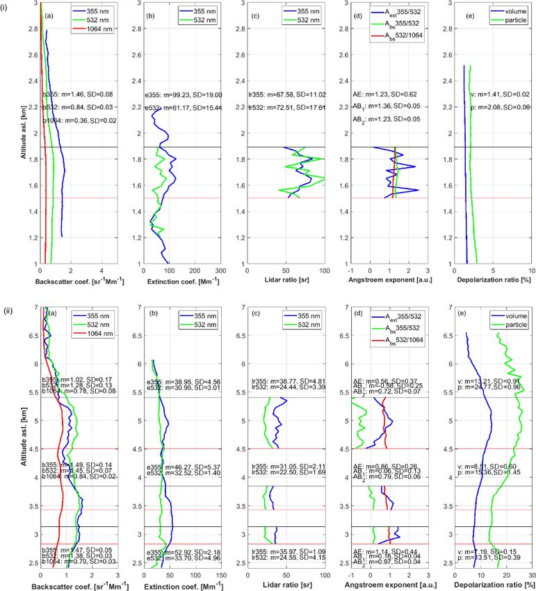
Figure 3 illustrates the vertical profiles of the aerosol op- on 30 July 2015 are also presented in Table 3. In particu-
tical properties, along with the mean values and standard de- lar, for the case of Kuopio, the LR355 values were found to
viations (inserted text) of the following: (3a) b355 , b532 , and be lower than those of LR532 , the Ångström exponent (both
b1064 (SR−1 Mm−1 ); (3b) e355 and e532 (Mm−1 ); (3c) LR355 extinction- and backscatter-related) was higher than 1.2, and
and LR532 (SR); (3d) Ae355/532 , Ab355/532 , and Ab532/1064 ; PLDR532 had low values (2216 M. Mylonaki et al.: Aerosol type classification analysis Figure 3. Vertical profiles of the following aerosol optical properties observed over (i) Kuopio (19:25 UTC) and (ii) Potenza (21:26 UTC) on 30 July 2015, along with their mean values and standard deviations (inserted text): (a) b355 , b532 , b1064 , (b) e355 , e532 , (c) LR355 , LR532 , (d) Ae355/532 , Ab355/532 , Ab532/1064 , (e) VDR532 , and PLDR532 . 24.8 ± 1.0 % (top layer), indicating coarse semi-depolarizing that reached Kuopio on that day at 1500 m a.s.l. (19:00 UTC) aerosols at lower altitudes (
M. Mylonaki et al.: Aerosol type classification analysis                                                                            2217

Table 3. Mean values of the intensive optical properties of aerosol layers observed on 30 July 2015 over Kuopio and Potenza.

    Site                 Height (km)      LR355 (SR)       LR532 (SR)        Ae355/532     Ab355/532     Ab532/1064    PLDR532 (%)
    Kuopio                   1.5–1.9    65.58 ± 11.02    72.51 ± 17.61     1.23 ± 0.62    1.36 ± 0.05   1.23 ± 0.05         2.1 ± 0.1
    Potenza (bottom)         2.8–3.1     35.97 ± 1.09     24.55 ± 4.15     1.14 ± 0.44    0.16 ± 0.04   0.97 ± 0.04        13.5 ± 0.4
    Potenza (middle)         3.4–3.9     31.05 ± 2.11     22.50 ± 1.69     0.86 ± 0.25    0.06 ± 0.13   0.79 ± 0.06        15.4 ± 1.5
    Potenza (top)            4.5–5.4     38.77 ± 4.81     24.44 ± 3.39     0.56 ± 0.37   -0.58 ± 0.25   0.72 ± 0.07        24.8 ± 1.0

These air masses started from northwestern Africa, remained              map as possible aerosol sources, which reduces the spatial
in the area almost 3 d, and then passed over southern Spain              accuracy of the classification method (Fig. 1). Therefore, we
before reaching Potenza. The aerosol layer observed over                 can see that the final results of the three methods (Fig. 5ia–
Potenza the same date and hour at 3800 m a.s.l. (middle layer,           c) are in good agreement concerning the layer observed over
Fig. 3ii, a–b) originated over the northern Atlantic Ocean at            Kuopio, although MD and SCAN can provide additional in-
a height of ∼ 5000 m a.s.l. 6 d before and slowly descended              formation on the constituents of the aerosol layer.
to lower altitudes before passing over northern Spain near                  On the other hand, the classification results for the aerosol
ground level (Fig. 4ii, 2). In the following 2 d, the air mass           layers observed over Potenza on t30 July 2015 are more
traveled at a height of 2000–4000 m a.s.l. from Spain to Italy           complex (Fig. 3ii). NATALI classified the lower and mid-
over the Mediterranean Sea before reaching Potenza.                      dle aerosol layers as marine/cc and the upper one as mineral
   Finally, the upper aerosol layer observed over Potenza at             mixtures/volcanic. However, regarding the lower and middle
5000 m a.s.l. (upper layer, Fig. 3ii, a–b) had a similar origin          aerosol layers, they are highly unlikely to be of marine ori-
as the previous one except the first 3 d of its journey when the         gin, as they are not affected by the sea spray at these heights
air masses traveled over the Atlantic Ocean at low altitudes             (>2.5 km a.s.l.). These erroneous classification results must
(
2218 M. Mylonaki et al.: Aerosol type classification analysis Figure 4. HYSPLIT (GDAS Meteorological Data) 6 d (144 h) air-mass backward trajectory ending on 30 July 2015 over the lidar stations in (i) Kuopio (62.74◦ N, 27.54◦ E) at 1500 m. a.s.l. (19:00 UTC) and (ii) Potenza (40.60◦ N, 15.72◦ E) at (1) 3000, (2) 4000, and (3) 5000 m a.s.l. (21:00 UTC) using the model vertical velocity as a vertical motion calculation method. The color bar indicates the trajectory’s height above mean sea level for each hour of its journey. comes obvious that an atmospheric dust model should be TALI and SCAN have many more. Finally, the SCAN algo- used synergistically with the SCAN results when we deal rithm (Fig. 6c) classified 37 % of the aerosol layers (36 lay- with air-mass backward trajectories passing over the south- ers) as 1 type, 30 % (29 layers) as aerosol mixtures, and 32 % ern Mediterranean Sea due to the vicinity of Sahara. (32 layers) as unknown types. 3 Results 3.1 Comparison of aerosol classification codes So far, 97 FT aerosol layers have been classified by the three In Fig. 7 we present a comparison of the classification results aforementioned classification algorithms. The results have obtained using the pairs of (a) NATALI and MD, (b) MD and been separated into aerosol layers according to aerosol types SCAN, and (c) SCAN and NATALI. The number of aerosol as follows: the 1 type (Fig. 6, blue) and mixture (Fig. 6, cyan) layers classified as indicated by the row i and the column j categories represent the aerosol layers that consist of one and is given inside each (i, j ) square. For example, the number two or more aerosol types, respectively. The other category of aerosol layers classified as being 1 type by MD but as a consists of cases that NATALI marked as aerosol type/cloud- mixture of aerosols by SCAN is shown inside the (1 type – contaminated (i.e., marine/cc), and finally, the unknown cat- mixture) square (there are 16 such cases for this example in egory (Fig. 6, yellow) consists of the cases for which the Fig. 7b). method was unable to identify the source of the observed In Fig. 7a it can be seen that the 45 cases classified as aerosol layers. All the aerosol types and mixtures considered unknown by MD were classified as 1 type (20 cases), a mix- by each algorithm are demonstrated in Table 1. ture (5 cases), or other (17 cases) by NATALI and 1 type It can be concluded that NATALI (Fig. 6a) is able to (12 cases) or a mixture (13 cases) by SCAN (Fig. 7b). Fur- classify the highest number of cases (94 cases), while MD thermore, it seems that MD is unable to discriminate the dif- (Fig. 6b) failed to classify a high number of cases (46 %) ferent aerosol types inside the other layers according to NA- with a lower percentage of aerosols classified as “mixture” TALI (Fig. 7a) and the mixture layers according to SCAN, types (5 %), which is a reasonable outcome given that the labeling them as 1 type (Fig. 7b), which is probably because MD scheme considers only two aerosol mixtures, while NA- only two aerosol mixtures are considered by MD. Concern- Atmos. Chem. Phys., 21, 2211–2227, 2021 https://doi.org/10.5194/acp-21-2211-2021
M. Mylonaki et al.: Aerosol type classification analysis                                                                                  2219

Figure 5. Aerosol layers observed over (i) Kuopio and (ii) Potenza at 3 (bottom), 3.8 (middle), and 5 km a.s.l. (top) on 30 July 2015 classified
by (a) NATALI, (b) MD, and (c) SCAN.

https://doi.org/10.5194/acp-21-2211-2021                                                     Atmos. Chem. Phys., 21, 2211–2227, 2021
2220                                                                     M. Mylonaki et al.: Aerosol type classification analysis

Figure 6. Percentages of classified aerosol layers by (a) NATALI, (b) MD, (c) SCAN. Blue: 1 type aerosol layers, cyan: mixtures, green:
other types, yellow: unknown constitution of aerosol layers.

Figure 7. Comparison between classified aerosol layers by (a) NATALI and MD, (b) MD and SCAN, and (c) SCAN and NATALI. The
number of classified aerosol layers as indicated by the i row and the j column is given inside each (i, j ) square.

ing the 29 unknown cases classified by SCAN, 20 of them               rameters are not within the accepted “borders” of the prede-
were also identified as unknown by MD (Fig. 7b), and they             fined classes of the algorithm. Concerning the 1 type aerosol
were almost equally separated into 1 type (12 cases) and              layers according to NATALI (Fig. 8b), MD would have pre-
other (16 cases) by NATALI (Fig. 7c).                                 dicted them correctly if the labeling of these layers by MD
                                                                      was achieved by considering a higher percentage of aerosol
3.1.1   NATALI versus MD                                              types, as the pie charts above each bar indicate (Fig. 8b). This
                                                                      does not seem to be the case for the dust type labeled by NA-
                                                                      TALI, to which MD gave a 40 % probability to be continen-
Figure 8a presents a comparison between the cases that MD             tal polluted, 30 % smoke, and only 30 % dust and mixed dust
classified as 1 type or a mixture against those classified as         (Fig. 8b). Concerning the mixture and other according to NA-
other by NATALI, while Fig. 8b shows the number of aerosol            TALI (Fig. 8c), it seems that MD found a high contribution of
layers that MD classified as unknown and NATALI as 1 type.            dust and mixtures of dust aerosols (approximately 50 %) in-
Finally, in Fig. 8c we present the number of aerosol layers           side these layers (yellow, orange, and dark red aerosol types
that MD classified as unknown and NATALI as a mixture or              according to the pie charts above the stems).
other. The pie charts above each bar (Fig. 8b) and each stem
(Fig. 8c) reveal the mean frequencies of each aerosol type as
calculated by MD.                                                     3.1.2   MD versus SCAN
   The inability of MD to classify the aerosol layers accord-
ing to NATALI’s classification (Fig. 8a) can be attributed            Figure 9a presents a comparison between the cases that were
to the characteristics of the aerosol layers not being well-          classified by MD as 1 type and as a mixture by SCAN, while
modeled by the algorithm, which means that the intensive pa-          Fig. 9b shows the number of aerosol layers classified by MD

Atmos. Chem. Phys., 21, 2211–2227, 2021                                                 https://doi.org/10.5194/acp-21-2211-2021
M. Mylonaki et al.: Aerosol type classification analysis 2221
Figure 8. (a) Comparison between the cases classified by MD as 1 type or mixture and as other by NATALI. (b) Number of aerosol layers
classified by MD as unknown and as 1 type by NATALI. (c) Number of aerosol layers classified by MD as unknown and as mixture or other
by NATALI. The pie charts above each bar and each stem reveal the mean frequencies of each aerosol type as calculated by MD.
as unknown and as 1 type by SCAN. Finally, Fig. 9c presents (b) SCAN classified as 1 type and NATALI as other, and
the number of aerosol layers classified by MD as unknown (c) SCAN classified as a mixture and NATALI as other.
and as a mixture or other by SCAN. The pie charts above From Fig. 10 it can be concluded that of the 12 cases that
each bar (Fig. 9b) and each stem (Fig. 9c) reveal the mean SCAN classified as continental polluted and smoke (cp + s),
frequencies of each aerosol type as calculated by MD. NATALI classified 6 of them as clean continental (cc), 4 as
The misclassification of an aerosol layer by MD compared continental polluted (cp) (Fig. 10a), and 2 as continental pol-
to the classification as a continental polluted and smoke layer luted and marine/cloud-contaminated (cp + m/cc) (Fig. 10c).
by SCAN (Fig. 9a) could again be attributed to the location Moreover, of the six cases that SCAN classified as continen-
of the observation compared to the location of the predefined tal polluted (cp), three of them were classified as continental
aerosol types for the MD classification algorithm, which de- polluted and marine or cloud-contaminated (cp + m/cc), two
pend on the aerosol optical properties of the studied layers. as marine/cloud-contaminated (m/cc), and only one as conti-
Additionally, it seems that the aerosol optical properties of nental polluted, smoke, and marine or cloud-contaminated
the mixture of continental polluted and smoke by SCAN are (cp + s + m/cc) by NATALI (Fig. 10b). It seems that the
attributed to either clean continental or continental polluted aerosol optical properties of this mixture are attributed to
aerosols by MD (Fig. 9a). From the cases that MD classified either the clean continental or continental polluted aerosol
as unknown, eight are classified as continental polluted (cp) types based on the NATALI classification.
by SCAN (Fig. 9b), while another six cases are classified
as continental polluted and smoke (cp + s) (Fig. 9c). Finally, 3.2 Aerosol optical properties
from these unknown cases by MD, there are another 11 cases
that SCAN classified as clean continental (two cases), dust The mean values of the aerosol optical properties derived
(one case), marine (one case; Fig. 9b), clean continental and from the NATALI, MD, and SCAN classification for each
marine (one case), continental polluted and clean continen- aerosol type are presented in Table 4 and discussed in this
tal (one case), continental polluted and marine (two cases), section. The correspondence between the aerosol types and
continental polluted, smoke, and marine (one case), or con- the terminology defined by the classification methods is pre-
tinental polluted, clean continental, and marine (two cases; sented in Table 1.
Fig. 9c).
3.2.1 Clean continental (cc) aerosols
3.1.3 SCAN versus NATALI Aerosol layers classified as clean continental by both
NATALI and MD present medium LR355 values (45–
Figure 10 presents a comparison between the cases that 46 ± 5 SR), medium to low LR532 values (37–39 ± 5 SR),
(a) SCAN classified as a mixture and NATALI as 1 type, medium Ab355/532 and Ab532/1064 values (1.0 ± 0.3), high
https://doi.org/10.5194/acp-21-2211-2021 Atmos. Chem. Phys., 21, 2211–2227, 20212222 M. Mylonaki et al.: Aerosol type classification analysis
Figure 9. (a) Comparison between the cases that were classified by MD as 1 type and as mixture by SCAN. (b) Number of aerosol layers
classified by MD as unknown and as 1 type by SCAN. (c) The number of aerosol layers classified by MD as unknown and as mixture or
other by SCAN. The pie charts above each bar and each stem reveal the mean frequencies of each aerosol type as calculated by MD.
Figure 10. Comparison between the cases classified by (a) SCAN as mixture and as 1 type by NATALI, (b) SCAN as 1 type and as other by
NATALI, and (c) SCAN as mixture and as other by NATALI.
Aeλ1/λ2 values (2.0 ± 0.3), and low PLDR values at 532 nm PLDR values at 532 nm (3 ± 1 %). On the other hand, the
(3 ± 1 %). These values are in accordance with others re- aerosol layers similarly classified by SCAN present medium
ported in previous studies concerning cc aerosols (Ansmann LR355 values (50 ± 6 SR) and LR532 values (49 ± 5 SR),
et al., 2001; Omar et al., 2009; Giannakaki et al., 2010). medium Ab355/532, Ab532/1064 , and Ae355/532 values (1.0–
1.5 ± 0.3), and low PLDR values at 532 nm (3 ± 1 %). These
3.2.2 Continental polluted (cp) aerosols values are also in accordance with those reported in previous
studies concerning this type of aerosol (Müller et al., 2007;
Aerosol layers classified as continental polluted by both Giannakaki et al., 2010; Gross et al., 2013; Burton et al.,
NATALI and MD present medium LR355 nm (57 ± 6 SR), 2013; Mattis et al., 2008). The similarity of these values to
slightly higher LR532 values (62 ± 7 SR), medium Ab355/532 , those of the clean continental aerosol type is the reason why
Ab532/1064 , and Ae355/532 values (1.1–1.4 ± 0.3), and low
Atmos. Chem. Phys., 21, 2211–2227, 2021 https://doi.org/10.5194/acp-21-2211-2021M. Mylonaki et al.: Aerosol type classification analysis 2223
Table 4. Mean values and standard deviations of aerosol optical properties according to each classification method.
Aerosol Method Clean Cont. Smoke Marine/ Dust + Cont. polluted + Cont. polluted + Cont. polluted +
types cont. polluted cl. cont. marine smoke marine dust + marine/
cl. cont.
No. of cases NAT 24 24 – 11 – – 14 7
MD 29 13 – – 4 – – –
SCAN – 22 5 – – 16 4 –
LR355 (SR) NAT 46.3 ± 5.0 57.5 ± 6.0 – 34.6 ± 3.5 – – 69.0 ± 11.0 41.4 ± 4.3
MD 44.9 ± 5.1 57.0 ± 6.4 – – 42.5 ± 4.4 – – –
SCAN – 50.2 ± 5.5 45.8 ± 4.7 – – 52.4 ± 7.9 45.3 ± 5.9 –
LR532 (SR) NAT 37.3 ± 3.7 61.6 ± 6.7 – 27.3 ± 3.4 – – 31.0 ± 5.3 43.1 ± 4.6
MD 38.9 ± 4.6 61.0 ± 6.9 – – 46.0 ± 4.7 – – –
SCAN – 49.2 ± 5.4 37.2 ± 4.0 – – 47.3 ± 7.1 54.8 ± 7.2 –
Ae355/532 NAT 2.0 ± 0.3 1.2 ± 0.3 – 1.7 ± 0.3 – – 0.9 ± 0.4 −0.1 ± 0.3
MD 1.6 ± 0.3 1.1 ± 0.3 – – −0.2 ± 0.2 – – –
SCAN – 1.5 ± 0.3 1.6 ± 0.3 – – 1.5 ± 0.4 0.3 ± 0.3 –
Ab355/532 NAT 1.1 ± 0.3 1.4 ± 0.3 – 0.9 ± 0.3 – – −1.2 ± 0.4 0.0 ± 0.3
MD 1.1 ± 0.3 1.2 ± 0.3 – – 0.0 ± 0.2 – – –
SCAN – 1.2 ± 0.3 0.9 ± 0.3 – – 0.8 ± 0.4 0.5 ± 0.3 –
Ab532/1064 NAT 1.2 ± 0.2 1.1 ± 0.2 – 1.0 ± 0.2 – – 1.3 ± 0.2 0.7 ± 0.1
MD 1.1 ± 0.2 1.1 ± 0.2 – – 0.7 ± 0.1 – – –
SCAN – 1.0 ± 0.2 1.3 ± 0.2 – – 1.3 ± 0.2 0.7 ± 0.2 –
PLDR ( %) NAT 3.4 ± 1.4 2.3 ± 0.7 – 4.1 ± 1.6 – – 2.7 ± 1.6 13.0 ± 4.4
MD 3.0 ± 1.2 2.7 ± 1.0 – – 15.2 ± 5.3 – – –
SCAN – 3.3 ± 1.3 2.7 ± 1.1 – – 4.0 ± 1.9 7.7 ± 3.8 –
it remains difficult to distinguish between these two aerosol 3.2.5 Dust and marine aerosols (d&m)
types.
Concerning the dust and marine mixture according to the
3.2.3 Smoke (s) aerosols MD algorithm classification, these aerosols showed medium
LR355 values (43 ± 4 SR), low LR532 values (46 ± 5 SR),
Smoke aerosol layers according to SCAN show medium small Ab355/532 , Ab532/1064 (0.0–0.7 ± 0.2), Ae355/532 val-
LR355 values (50 ± 5 SR), medium to small LR532 values ues (−0.2 ± 0.2), and medium PLDR532 values (15 ± 5 %).
(37 ± 4 SR), medium Ab355/532 and Ab532/1064 values (0.9– These values indicate large and depolarizing aerosol parti-
1.3 ± 0.3), medium to high Ae355/532 values (1.6 ± 0.3), and cles, confirming the type of these particles as a mixture of
low PLDR values at 532 nm (3 ± 1 %). These values are in dust and marine ones, according to Burton et al. (2012) and
accordance with those reported in previous studies concern- Papagiannopoulos et al. (2016).
ing this type of aerosol (Wandinger et al., 2002; Müller et al.,
3.2.6 Continental polluted and smoke (cp&s) aerosols
2005, 2007; Burton et al., 2013; Baars et al., 2012; Balis, et
al., 2003; Papanikolaou, et al., 2020). Again, the similarity of The continental polluted and smoke mixed aerosols clas-
these values to those of the clean continental and continental sified according to SCAN showed medium LR355 values
polluted aerosol types is the reason why it remains difficult (52 ± 8 SR), medium LR532 values (47 ± 7 SR), medium
to distinguish between these three aerosol types. Ab355/532 and Ab532/1064 values (0.8–1.3 ± 0.4), high val-
ues of Ae355/532 (1.5 ± 0.4), and low values of PLDR532
3.2.4 Marine/cloud-contaminated (m/cc) aerosols (4 ± 2 %). The medium LR355 and LR532 values indicate
continental polluted aerosols (Müller et al., 2007; Gian-
Aerosol layers classified as marine/cloud-contaminated by nakaki et al., 2010; Gross et al., 2013; Burton et al., 2013;
NATALI showed low values of LR355 (35 ± 4 SR), even Papanikolaou, et al., 2020), while the high Ae355/532 values
lower LR532 values (27 ± 3 SR), small to medium Ab355/532 indicate smoke aerosols (Wandinger et al., 2002; Müller et
and Ab532/1064 values (0.9-1.0 ± 0.3), increased Ae355/532 al., 2005).
values (1.7 ± 0.3), and low PLDR532 values (4 ± 2 %). These
values are in accordance with those reported by Cattrall
et al. (2005), Burton et al. (2012, 2013), and Dawson, et
al. (2015) concerning marine aerosols.
https://doi.org/10.5194/acp-21-2211-2021 Atmos. Chem. Phys., 21, 2211–2227, 20212224 M. Mylonaki et al.: Aerosol type classification analysis
3.2.7 Continental polluted and marine (cp&m) aerosols regions and a number of additional criteria, as analytically
presented.
The continental polluted and marine mixture accord- We concluded that NATALI showed a lower percentage
ing to NATALI showed a large difference between the (4 %) of unclassified layers. When compared to MD, NA-
LR355 and LR532 values, with the latter being smaller TALI’s X or cloud-contaminated aerosol layers (where X is
(LR355 = 69 ± 11, LR532 = 31 ± 5.3 SR). The Ae355/532 , either an aerosol type or a mixture) are classified by MD as
Ab355/532 , and PLDR at 532 nm showed low values clean continental layers, except when X is a mixture of dust
(0.9 ± 0.4, −1.2 ± 0.4, 2.7 ± 1.6, respectively), while the aerosols. When compared, SCAN’s continental polluted and
Ab532/1064 showed large values (1.3 ± 0.2). SCAN showed smoke layers are classified by NATALI as either clean conti-
medium LR355 values (45 ± 6 SR), increased LR532 values nental or continental polluted.
(55 ± 7 SR), low Ab355/532 , Ab532/1064 , and Ae355/532 val- Furthermore, we found that MD was unable to classify al-
ues (0.3–0.7 ± 0.3), and low PLDR532 values (8 ± 4 %). The most 50 % of the layers under study. Compared to NATALI,
low PLDR values are indicative of non-depolarizing aerosols these layers either belong to one single aerosol type or to
such as continental polluted (Müller et al., 2007; Giannakaki aerosol mixtures. Concerning MD’s unknown category and
et al., 2010; Gross et al., 2013; Burton et al., 2013) and NATALI’s one single aerosol type, we showed that MD’s
marine aerosols (Gross et al., 2011; Burton et al., 2012, mean percentages predict the aerosol type of each layer quite
2013; Gross et al., 2013). Additionally, the low Ab355/532 , well, even though this aerosol type is not chosen by the clas-
Ab532/1064 , and Ae355/532 values are indicative of coarse- sification process of MD. Concerning MD’s unknown and
mode aerosols such as marine, while the increased LR532 NATALI’s mixture categories, the MD algorithm revealed an
values are more indicative of continental polluted aerosols increased contribution of dust aerosols (approximately 50 %)
rather than marine ones. inside the studied aerosol layers. Compared to SCAN, MD’s
unknown layers are mainly either continental polluted or
3.2.8 Continental polluted, dust, and marine or clean continental polluted and smoke. Finally, SCAN’s continen-
continental (cp&d&m/cc) aerosols tal polluted and smoke layers are classified by MD as either
clean continental or continental polluted.
Finally, the continental polluted, dust, and marine or cloud- We found that the SCAN code successfully managed to
contaminated aerosol mixture classified by NATALI showed classify more than 50 % of the layers studied either as a sin-
medium LR355 values (41 ± 4 SR), medium LR532 values gle aerosol type or as mixtures of different aerosols. Being
(43 ± 5 SR), low Ab355/532 , Ab532/1064 , and Ae355/532 values independent of aerosol optical properties, SCAN provides
(−0.1–0.7 ± 0.3), and medium PLDR532 values (13 ± 4 %). the advantage that its classification process is not affected
Here, the medium PLDR values are indicative of dust mix- by overlapping values of the optical properties representing
tures (Gross et al., 2011, 2016; Burton et al., 2013), while the more than one aerosol type (clean continental, continental
low Ab355/532 , Ab532/1064 , and Ae355/532 values are indicative polluted, smoke). Furthermore, it has no limitations concern-
of coarse-mode aerosols, such as dust and marine. ing its ability to classify aerosol mixtures, an advantage that
arises from the air-mass trajectory analysis and the relevant
aerosol sources on the ground. Finally, it can be useful for
4 Conclusions all types of lidar systems (independently of the number of
channels used) and for other network-based systems (radar
In this study, we compared three independent aerosol clas- profilers, sun photometers).
sification methods: a neural network aerosol typing algo-
rithm, the Mahalanobis distance automatic aerosol type clas-
sification, and a source classification analysis using 97 free Data availability. The aerosol lidar profiles used in this study are
tropospheric aerosol layers from four EARLINET stations available upon registration from the EARLINET web page at https:
(Bucharest, Kuopio, Leipzig, and Potenza) from 2014–2018. //data.earlinet.org/earlinet/login.zul (Pappalardo et al., 2014).
NATALI is an automated aerosol layer classification neural
network depending on the aerosol optical properties (3β +
2α + 1δ) directly obtained from the EARLINET database. Author contributions. DN, NP, and EG distributed the NATALI,
MD, and SCAN algorithms, respectively. CAP created algorithms
MD is an automated aerosol layer classification algorithm
that produced the maps presented in this work. EG had the idea for
depending on the mean values of the aerosol optical prop-
this paper. MM upgraded the SCAN algorithm, collected the lidar
erties (Ae355/1064 , LR532 , LR532 / LRλ355 , PLDR532 , and data, made the comparison, analyzed the results, and wrote the pa-
Ab1064/532 ) of the probed atmospheric layers. SCAN, intro- per. All authors participated in scientific discussions on this study
duced for the first time in this study, is based on the automa- and reviewed and edited the paper during its preparation process.
tization of the typical classification method, while its classi-
fication procedure is based on the amount of time that an air
parcel spends over specific pre-characterized aerosol source
Atmos. Chem. Phys., 21, 2211–2227, 2021 https://doi.org/10.5194/acp-21-2211-2021M. Mylonaki et al.: Aerosol type classification analysis 2225
Competing interests. The authors declare that they have no conflict Portuguese coast, J. Geophys. Res. Atmos., 106, 20725–20733,
of interest. https://doi.org/10.1029/2000JD000091, 2001.
Baars, H., Ansmann, A., Althausen, D., Engelmann, R., Heese, B.,
Mller, D., Artaxo, P., Paixao, M., Pauliquevis, T., and Souza,
Special issue statement. This article is part of the special issue R.: Aerosol profiling with lidar in the Amazon Basin during
“EARLINET aerosol profiling: contributions to atmospheric and the wet and dry season, J. Geophys. Res. Atmos., 117, 1–16,
climate research”. It is not associated with a conference. https://doi.org/10.1029/2012JD018338, 2012.
Balis, D. S., Amiridis, V., Zerefos, C., Gerasopoulos, E., An-
dreae, M., Zanis, P., Kazantzidis, A., Kazadzis, S., and Pa-
Acknowledgements. The authors acknowledge support through payannis, A.: Raman lidar and sunphotometric measurements
ACTRIS under grant agreement no. 262254 from the European of aerosol optical properties over Thessaloniki, Greece during
Commission Seventh Framework Programme (FP7/2007–2013) a biomass burning episode, Atmos. Environ., 37, 4529–4538,
and ACTRIS-2 under grant agreement no. 654109 from the Horizon https://doi.org/10.1016/S1352-2310(03)00581-8, 2003.
2020 research and innovation program of the European Commis- Basart, S., Pérez, C., Nickovic, S., Cuevas, E., and Bal-
sion. The authors acknowledge EARLINET for providing aerosol dasano, J.: Development and evaluation of the BSC-
lidar profiles available at https://data.earlinet.org/ (last access: 1 Au- DREAM8b dust regional model over Northern Africa, the
gust 2020). The authors gratefully acknowledge the NOAA Air Mediterranean and the Middle East, Tellus B, 64, 18539,
Resources Laboratory (ARL) for the provision of the HYSPLIT https://doi.org/10.3402/tellusb.v64i0.18539, 2012.
transport and dispersion model as well as the READY website Belegante, L., Nicolae, D., Nemuc, A., Talianu, C., and Derognat,
(http://www.ready.noaa.gov, last access: 1 August 2020) used in C.: Retrieval of the boundary layer height from active and passive
this publication. We acknowledge the use of data products and im- remote sensors. Comparison with a NWP model, Acta Geophys.,
agery from the Land, Atmosphere Near-real-time Capability for 62, 276–289, https://doi.org/10.2478/s11600-013-0167-4, 2014.
EOS (LANCE) system operated by NASA’s Earth Science Data Boucher, O., Randall, D., Artaxo, P., Bretherton, C., Feingold, G.,
and Information System (ESDIS) with funding provided by NASA Forster, P., Kerminen, V.-M., Kondo, Y., Liao, H., Lohmann, U.,
headquarters. Rasch, P., Satheesh, S. K., Sherwood, S., Stevens, B., and Zhang,
X. Y.: Clouds and Aerosols, in: Climate Change 2013: The Phys-
ical Science Basis. Contribution of Working Group I to the Fifth
Assessment Report of the Intergovernmental Panel on Climate
Financial support. This research has been supported by the Hel-
Change, edited by: Stocker, T. F., Qin, D., Plattner, G.-K., Tig-
lenic Foundation for Research and Innovation (grant no. 669) and
nor, M., Allen, S. K., Boschung, J., Nauels, A., Xia, Y., Bex,
the PANhellenic infrastructure for Atmospheric Composition and
V., and Midgley, P. M., Cambridge University Press, Cambridge,
climatE change (grant no. MIS 5021516), which is implemented
United Kingdom and New York, NY, USA, 2013.
under the action “Reinforcement of the Research and Innovation
Burton, S. P., Ferrare, R. A., Hostetler, C. A., Hair, J. W., Rogers, R.
Infrastructure” funded by the operational program “Competitive-
R., Obland, M. D., Butler, C. F., Cook, A. L., Harper, D. B., and
ness, Entrepreneurship and Innovation” (NSRF 2014–2020), and
Froyd, K. D.: Aerosol classification using airborne High Spec-
co-financed by Greece and the European Union (European Regional
tral Resolution Lidar measurements-methodology and examples,
Development Fund).
Atmos. Meas. Tech., 5, 73–98, https://doi.org/10.5194/amt-5-73-
2012, 2012.
Burton, S. P., Ferrare, R. A., Vaughan, M. A., Omar, A. H.,
Review statement. This paper was edited by Eduardo Landulfo and Rogers, R. R., Hostetler, C. A., and Hair, J. W.: Aerosol
reviewed by three anonymous referees. classification from airborne HSRL and comparisons with the
CALIPSO vertical feature mask, Atmos. Meas. Tech., 6, 1397–
1412, https://doi.org/10.5194/amt-6-1397-2013, 2013.
Cattrall, C., Reagan J., Thome K., and Dubovik O.: Variabil-
ity of aerosol and spectral lidar and backscatter andextinc-
References tion ratios of key aerosol types derived from selected Aerosol
Robotic Network locations, J. Geophys. Res., 11, D10S11,
Althausen, D., Engelmann, R., Baars, H., Heese, B., Ansmann, https://doi.org/10.1029/2004JD005124, 2005.
A., Müller, D., and Komppula, M.: Portable raman lidar pol- Davies, D. K., Ilavajhala, S., Wong, M. M., and Justice, C. O.: Fire
lyxt for automated profiling of aerosol backscatter, extinction, information for resource management system: Archiving and dis-
and depolarization, J. Atmos. Ocean. Technol., 26, 2366–2378, tributing MODIS active fire data, IEEE T. Geosci. Remote Sens.,
https://doi.org/10.1175/2009JTECHA1304.1, 2009. 47, 72–79, https://doi.org/10.1109/TGRS.2008.2002076, 2009.
Amiridis, V., Giannakaki, E., Balis, D. S., Gerasopoulos, E., Dawson, K. W., Meskhidze, N., Josset, D., and Gassó, S.: Space-
Pytharoulis, I., Zanis, P., Kazadzis, S., Melas, D., and Zerefos, borne observations of the lidar ratio of marine aerosols, At-
C.: Smoke injection heights from agricultural burning in Eastern mos. Chem. Phys., 15, 3241–3255, https://doi.org/10.5194/acp-
Europe as seen by CALIPSO, Atmos. Chem. Phys., 10, 11567– 15-3241-2015, 2015.
11576, https://doi.org/10.5194/acp-10-11567-2010, 2010. Draxler, R. R. and Hess, G. D.: An overview of HYSPLIT_4 mod-
Ansmann, A., Wagner, F., Althausen, D., Müller, D., Herber, A., elling system for trajectories, dispersion and deposition, Aust.
and Wandinger, U.: European pollution outbreaks during ACE Met. Mag., 47, 295–308, 2013.
2: Lofted aerosol plumes observed with Raman lidar at the
https://doi.org/10.5194/acp-21-2211-2021 Atmos. Chem. Phys., 21, 2211–2227, 20212226 M. Mylonaki et al.: Aerosol type classification analysis Freudenthaler, V., Esselborn, M., Wiegner, M., Heese, B., Tesche, dar over central Europe in 2008–2009, J. Geophys. Res.-Atmos., M., Ansmann, A., Müller, D., Althausen, D., Wirth, M., Fix, A., 115, 1–9, https://doi.org/10.1029/2009JD013472, 2010. Ehret, G., Knippertz, P., Toledano, C., Gasteiger, J., Garham- Mishchenko, M. I., Travis, L. D., and Mackowski, D. W.: T- mer, M., and Seefeldner, M.: Depolarization ratio profiling matrix computations of light scattering by nonspherical parti- at several wavelengths in pure Saharan dust during SAMUM cles: A review, J. Quant. Spectrosc. Radiat. Transf., 55, 535–575, 2006, Tellus B, 61, 165–179, https://doi.org/10.1111/j.1600- https://doi.org/10.1016/0022-4073(96)00002-7, 1996. 0889.2008.00396.x, 2009. Müller, D., Mattis, I., Wandinger, U., Ansmann, A., Althausen, D., Georgoulias, A. K., van der A, R. J., Stammes, P., Boersma, and Stohl, A.: Raman lidar observations of aged Siberian and K. F., and Eskes, H. J.: Trends and trend reversal detection Canadian forest-fire smoke in the free troposphere over Germany in 2 decades of tropospheric NO2 satellite observations, At- in 2003: Microphysical particle characterization, J. Geophys. mos. Chem. Phys. 19, 6269–6294, https://doi.org/10.5194/acp- Res., 110, D17201, https://doi.org/10.1029/2004JD005756, 19-6269-2019, 2019. 2005. Giannakaki, E., Balis, D. S., Amiridis, V., and Zerefos, C.: Müller, D., Ansmann, A., Mattis, I., Tesche, M., Wandinger, U., Al- Optical properties of different aerosol types: Seven years thausen, D., and Pisani, G.: Aerosol-type-dependent lidar ratios of combined Raman-elastic backscatter lidar measurements observed with Raman lidar, J. Geophys. Res.-Atmos., 112, 1–11, in Thessaloniki, Greece, Atmos. Meas. Tech., 3, 569–578, https://doi.org/10.1029/2006JD008292, 2007. https://doi.org/10.5194/amt-3-569-2010, 2010. Nemuc, A., Vasilescu, J., Talianu, C., Belegante, L., and Nico- Giannakaki, E., Van Zyl, P. G., Müller, D., Balis, D., and Komppula, lae, D.: Assessment of aerosol’s mass concentrations from M.: Optical and microphysical characterization of aerosol layers measured linear particle depolarization ratio (vertically re- over South Africa by means of multi-wavelength depolarization solved) and simulations, Atmos. Meas. Tech., 6, 3243–3255, and Raman lidar measurements, Atmos. Chem. Phys., 16, 8109– https://doi.org/10.5194/amt-6-3243-2013, 2013. 8123, https://doi.org/10.5194/acp-16-8109-2016, 2016. Nicolae, D., Talianu, C., Ionescu, C., Ciobanu, M., and Ciuciu, J.: Giglio, L., Descloitres, J., Justice, C. O., and Kaufman, Y. J.: An en- Aerosol statistics and pollution forecast based on lidar measure- hanced contextual fire detection algorithm for MODIS, Remote ments in Bucharest, Romania, Lidar Technol. Tech. Meas. At- Sens. Environ., 87, 273–282, https://doi.org/10.1016/S0034- mos. Remote Sens., 59840, https://doi.org/10.1117/12.627727, 4257(03)00184-6, 2003. 2005. Gross, S., Esselborn, M., Weinzierl, B., Wirth, M., Fix, A., and Pet- Nicolae, D., Talianu, C., Ciuciu, J., Ciobanu, M., and Babin, V.: zold, A.: Aerosol classification by airborne high spectral reso- LIDAR monitoring of aerosols loading over Bucharest, J. Opto- lution lidar observations, Atmos. Chem. Phys., 13, 2487–2505, electron. Adv. Mater., 8, 238–242, 2006. https://doi.org/10.5194/acp-13-2487-2013, 2013. Nicolae, D., Nemuc, A., Müller, D., Talianu, C., Vasilescu, J., Bel- Hamill, P., Piedra, P., and Giordano, M.: Simulated polarization egante, L., and Kolgotin, A.: Characterization of fresh and aged as a signature of aerosol type, Atmos. Environ., 224, 117348, biomass burning events using multiwavelength Raman lidar and https://doi.org/10.1016/j.atmosenv.2020.117348, 2020. mass spectrometry, J. Geophys. Res.-Atmos., 118, 2956–2965, Ho, S. P., Peng, L., Anthes, R. A., Kuo, Y. H., and Lin, H. C.: Ma- https://doi.org/10.1002/jgrd.50324, 2013. rine boundary layer heights and their longitudinal, diurnal, and Nicolae, D., Talianu, C., Vasilescu, J., Nicolae, V., and interseasonal variability in the southeastern Pacific using COS- Stachlewska, I. S.: Strengths and limitations of the NA- MIC, CALIOP, and radiosonde data, J. Clim., 28, 2856–2872, TALI code for aerosol typing from multiwavelength https://doi.org/10.1175/JCLI-D-14-00238.1, 2015. Raman lidar observations, EPJ Web Conf., 176, 1–4, Hobbs, P. V.: Aerosol-cloud interactions, in: Aerosol-Cloud- https://doi.org/10.1051/epjconf/201817605005, 2018a. Climate Interactions, Academic, San Diego, California, 1993. Nicolae, D., Vasilescu, J., Talianu, C., Binietoglou, I., Nicolae, V., Justice, C. O., Giglio, L., Korontzi, S., Owens, J., Morisette, J. T., Andrei, S., and Antonescu, B.: A neural network aerosol-typing Roy, D., Descloitres, J., Alleaume, S., Petitcolin, F., and Kauf- algorithm based on lidar data, Atmos. Chem. Phys., 18, 14511– man, Y.: The MODIS fire products, Remote Sens. Environ., 14537, https://doi.org/10.5194/acp-18-14511-2018, 2018b. 83, 244–262, https://doi.org/10.1016/S0034-4257(02)00076-7, Omar, A. H., Winker, D. M., Kittaka, C., Vaughan, M. A., 2002. Liu, Z., Hu, Y., Trepte, C. R., Rogers, R. R., Ferrare, R. Kaufman, Y. J., Justice, C. O., Flynn, L .P., Kendall, J. D., Prins, A., Lee, K. P., Kuehn, R. E., and Hostetler, C. A.: The E. M., Giglio, L., Ward, D. E., Menzel, W. P., and Setzer, A. W.: CALIPSO automated aerosol classification and lidar ratio se- Potential global fire monitoring from EOS-MODIS, J. Geophys. lection algorithm, J. Atmos. Ocean. Technol., 26, 1994–2014, Res., 103, 32215–32238, 1998. https://doi.org/10.1175/2009JTECHA1231.1, 2009. Koepke, P., Hess, M., Schult, I., and Shettle, E. P.: Global Aerosol Papagiannopoulos, N., Mona, L., Alados-Arboledas, L., Amiridis, Data Set, Report No. 243, MPI Hamburg, Germany, 44 pp., 1997. V., Baars, H., Binietoglou, I., Bortoli, D., D’Amico, G., Madonna, F., Amodeo, A., Boselli, A., Cornacchia, C., Cuomo, Giunta, A., Luis Guerrero-Rascado, J., Schwarz, A., Pereira, V., D’Amico, G., Giunta, A., Mona, L., and Pappalardo, S., Spinelli, N., Wandinger, U., Wang, X., and Pappalardo, G.: CIAO: The CNR-IMAA advanced observatory for at- G.: CALIPSO climatological products: Evaluation and sugges- mospheric research, Atmos. Meas. Tech., 4, 1191–1208, tions from EARLINET, Atmos. Chem. Phys., 16, 2341–2357, https://doi.org/10.5194/amt-4-1191-2011, 2011. https://doi.org/10.5194/acp-16-2341-2016, 2016. Mattis, I., Siefert, P., Müller, D., Tesche, M., Hiebsch, A., Kanitz, Papagiannopoulos, N., Mona, L., Amodeo, A., D’Amico, G., T., Schmidt, J., Finger, F., Wandinger, U., and Ansmann, A.: Vol- Gumà Claramunt, P., Pappalardo, G., Alados-Arboledas, L., Luís canic aerosol layers observed with multiwavelength Raman li- Guerrero-Rascado, J., Amiridis, V., Kokkalis, P., Apituley, A., Atmos. Chem. Phys., 21, 2211–2227, 2021 https://doi.org/10.5194/acp-21-2211-2021
You can also read