Climate change impact on the potential geographical distribution of two invading Xylosandrus ambrosia beetles - Nature
←
→
Page content transcription
If your browser does not render page correctly, please read the page content below
www.nature.com/scientificreports
OPEN Climate change impact
on the potential geographical
distribution of two invading
Xylosandrus ambrosia beetles
T. Urvois1*, M. A. Auger‑Rozenberg1, A. Roques1, J. P. Rossi2,3 & C. Kerdelhue2,3
Xylosandrus compactus and X. crassiusculus are two polyphagous ambrosia beetles originating from
Asia and invasive in circumtropical regions worldwide. Both species were recently reported in Italy
and further invaded several other European countries in the following years. We used the MaxEnt
algorithm to estimate the suitable areas worldwide for both species under the current climate. We
also made future projections for years 2050 and 2070 using 11 different General Circulation Models,
for 4 Representative Concentration Pathways (2.6, 4.5, 6.0 and 8.5). Our analyses showed that X.
compactus has not been reported in all potentially suitable areas yet. Its current distribution in Europe
is localised, whereas our results predicted that most of the periphery of the Mediterranean Sea and
most of the Atlantic coast of France could be suitable. Outside Europe, our results also predicted
Central America, all islands in Southeast Asia and some Oceanian coasts as suitable. Even though our
results when modelling its potential distribution under future climates were more variable, the models
predicted an increase in suitability poleward and more uncertainty in the circumtropical regions. For
X. crassiusculus, the same method only yielded poor results, and the models thus could not be used
for predictions. We discuss here these results and propose advice about risk prevention and invasion
management of both species.
Biological invasions are one of the main threats to biodiversity worldwide, and their magnitude has increased
over the last decades with global c hange1. Indeed, climate change alters environmental parameters such as tem-
perature and precipitation patterns and tends to increase the frequency of extreme events2. These alterations
can decrease ecosystems’ resistance and resilience to invasion3,4, increase species invasiveness5 and initiate range
shifts6. Human transportation, whether intentional or unintentional, also plays a significant role in shifting spe-
ispersion7, including in normally out-of-reach areas. Moreover, it also
cies’ range by increasing species passive d
increases the propagule pressure (i.e. the number of individuals introduced and the number of introduction
events), known to affect establishment probability and ultimately the number of invasive species8. Two major
challenges of trans-boundary species management are (1) to detect target species at the earliest possible stage
and (2) to quickly provide specific actions to regulate or eradicate t hem9. To do so, it is necessary to plan ahead
and perform pest risk analyses, which aims at assessing species’ invasion risk considering various biological and
environmental characteristics in a given area.
Species distribution modelling (SDM) aims at predicting environment suitability, and thus the potential dis-
tribution of a given species in a determined range. SDM is an increasingly important tool for decision-makers
when prioritising biodiversity conservation efforts or dealing with invasive s pecies10. For the latter, the estimation
of habitat suitability can be used to decide how and where to set up detection methods and thus improve early
detection probability. SDM uses the relationship between environmental descriptors and the species’ observed
distribution to estimate its realised niche11, which is used to extrapolate habitat suitability outside of the cur-
rent species’ range. SDM is also an interesting tool to assess the potential effects of climate change on species
distribution12. To simulate future climate, scientists rely on Global Circulation Models (GCMs), which attempt
to account for all the physical and chemical processes influencing climate, such as ocean, atmosphere, land and
sea ice. To predict the effect of greenhouse gases concentration on future climate, each GCM can be run using
different radiative forcing scenarios, represented by different Representative Concentration Pathways (RCPs).
1
INRAE, URZF, 45045 Orléans, France. 2UMR CBGP, INRAE, CIRAD, IRD, Institut Agro, Université Montpellier,
Montpellier, France. 3These authors contributed equally: J. P. Rossi and C. Kerdelhue. *email: teddy.urvois@
inrae.fr
Scientific Reports | (2021) 11:1339 | https://doi.org/10.1038/s41598-020-80157-9 1
Vol.:(0123456789)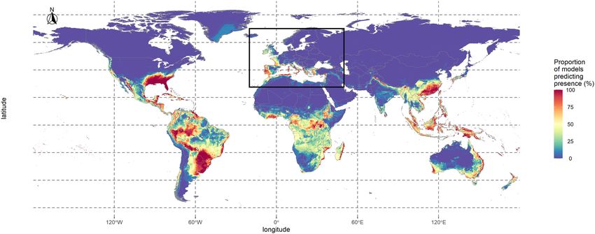
www.nature.com/scientificreports/
Four RCPs were used for the IPCC 5th Assessment Report13, ranging from the most optimistic one (RCP2.6) to
the least optimistic (RCP8.5). Different GCMs are available that all represent a possible future, which we cannot
discriminate from. Therefore, GCM selection can potentially affect the results of future distribution modelling14,
being the primary source of variability between models after the algorithm choice15. However, this step is often
overlooked and the GCM choice made by default or not j ustified12. When facing biological invasion, it is equally
important to determine which areas are suitable and could be threatened, and which ones are consistently pre-
dicted as unsuitable. In this regard, using several GCMs allows to explore the uncertainty of SDM predictions
and to gain confidence on suitability estimates.
Bark and ambrosia beetles (Coleoptera:Curculionidae:Scolytinae) are considered as one of the most successful
groups of invasive species16 and represent an increasing concern worldwide17. They are hard to detect as they are
usually minute insects, and can travel long distances unnoticed, hidden in wood packaging or living plants18.
Within this group, the species of the genus Xylosandrus are especially threatening. Two of them, X. crassiusculus
and X. compactus, native of Southeast Asia, are known invaders worldwide and share similar invasion histories.
Both have been detected outside of their native range more than one century ago in Madagascar before spread-
ing to continental Africa and later in the New World. X. compactus was detected in North America in 1941 in
Florida19, in Hawaii in 1 96420 and in South America in Brazil in 1 97921. X. crassiusculus was first detected in
Hawaii in 1 95022, in North America in South Carolina in 1 97423 and in South America in Argentina in 2 00124.
Both species were recently reported from Europe where they were first detected in Italy, X. crassiusculus in 2 00325
and X. compactus 201126, before being detected in France in 2014 and 2 01527, respectively. X. crassiusculus was
then detected in 2016 in S pain28 and in 2017 in S lovenia29 whilst X. compactus was detected in 2019 in G reece30
31
and on the island of Majorca in Spain . As other ambrosia beetles, their ecological characteristics tend to favour
invasion. They are xylomycetophagous and feed on symbiotic fungi carried in a specialised structure in their body
called mycangium. This feature allows them to attack a broader range of host tree32, which is known to be a major
reason for their success as invaders33. More, siblings mate directly in the maternal gallery, which could allow
a single mated female to establish a population. Therefore, they presumably avoid classical detrimental effects
of deterministic processes such as mate-finding Allee effect or inbreeding as they are haplodiploid and evolved
under inbred mating strategies34. Both species originate from subtropical areas and succeeded in invading tropical
and subtropical regions in a first step. However, both are now established under temperate and Mediterranean
climates, as X. crassiusculus is now established as far North as South Canada35 and was intercepted several times
in the Netherlands during the last decade36. We can thus assume that both species are quite plastic, although
little is known about their precise ecological requirements.
The first goal of this study was to estimate the potential distribution of both species, with a particular focus
on Europe that was recently invaded and where the distribution range of both species is still fairly limited. It is
thus now necessary to identify the regions where these invaders still do not occur but could be at risk, to antici-
pate their expansion and develop preventive management strategies. The second goal of this study is to make
predictions about the effect of climate change on both species’ potential distributions in the near future to assess
whether some new areas could become suitable or conversely if some area could stay or become unsuitable. To
answer both objectives, we performed SDM on X. crassiusculus and X. compactus using MaxEnt algorithm (1)
on current and (2) on future climate models for 2050 and 2070 using 11 GCMs and 4 RCPs. As both species have
similar ecological characteristics and a parallel invasion history, we expect that they could threaten the same
regions. As hypothesised by Kirkendall and F accoli17, the Mediterranean seems particularly favourable for inva-
sive species with a rich biodiversity and milder winters than the rest of Europe. It corresponds to a biodiversity
hotspot that is expected to be particularly susceptible to climate c hange37. Assessing the risk of further invasions
in this area is thus of prime importance.
Material and methods
Occurrence data and environmental variables. We collected worldwide occurrence records of X.
crassiusculus and X. compactus from the scientific literature (Supplementary Table S1), the Global Biodiversity
Information Facility (GBIF) and direct observations up until the 13th of September 2019. Once removed the
localities where the species was not proven to be established, we were left with respectively 781 and 323 records
for X. crassiusculus and X. compactus. We then removed duplicated data, by withdrawing all but one occurrence
record per pixel of the climate raster (see below), and ended with 311 occurrences for X. crassiusculus (33% in its
native area) and 205 occurrences for X. compactus (30% in its native area) (Fig. 1).
We used environmental variables available from the Worldclim database (version 2.0)38, corresponding to the
average climate values for 1970–2000, with a resolution of 2.5 arc-min (≈4.5 km at the equator). We selected a
priori 11 variables assumed to be potential drivers of X. crassiusculus and X. compactus distributions. Five were
descriptors of the temperature: the temperature seasonality (bio4) and the average temperatures of the wettest,
driest, hottest and coldest quarters (respectively bio8, bio9, bio10 and bio11). The remaining 6 variables were
the annual precipitations (bio12), the precipitation seasonality (bio15), and the average precipitations of the wet-
test, driest, hottest and coldest quarters (respectively bio16, bio17, bio18, bio19). Model overfitting is an i ssue39
especially when one aims at using the model to assess future potential distribution40. To reduce this issue, we
grouped the environmental descriptors by groups of 4 or 5 to produce 126 environmental datasets. Modelling
was performed with small sets of variables, hence preventing overfitting.
Modelling. Because the Xylosandrus species under study are invaders in various regions of the world, their
spatial range is in constant evolution. In such a non-equilibrium situation, it is very hard to identify locations
where the species is absent because environmental conditions are unfavourable (i.e. true absence) rather than
because of (transient) dispersal limitations. In such a situation, presence-only algorithms are r ecommended10.
Scientific Reports | (2021) 11:1339 | https://doi.org/10.1038/s41598-020-80157-9 2
Vol:.(1234567890)www.nature.com/scientificreports/
Figure 1. Occurrence data used in the present study of (a) Xylosandrus compactus (n = 205) and (b) Xylosandrus
crassiusculus (n = 311) after duplicate removal. The maps were generated using R 4.0.0 (https://cran.r-proje
ct.org/).
We thus used the MaxEnt algorithm41, which has been widely adopted in species modelling, notably in biologi-
cal invasions surveys42. To make predictions, MaxEnt relies on presence-only data and background points (i.e.
locations where the species’ presence in unknown used as a contrast against presence occurrences).
A first step of the modelling framework consisted in selecting the combinations of climate descriptors that
led to the MaxEnt models that best predicted European occurrences when calibrated using occurrences from
other regions of the world (see e.g. Godefroid et al.42 for an example of such a strategy). To do so, we removed
the European occurrences from the datasets of each species, and randomly sampled 80% of the remaining occur-
rence records to train the model. The remaining 20% of records were used to evaluate the model. To characterise
the background environment, 10,000 background points were randomly generated in a wide area representative
of the species’ habitat. We did this for 10 replicates for each of the 126 environmental datasets used for each
species. We retained a dataset when at least 5 replicates performed (1) an Area Under Curve (AUC) > 0.8, (2) a
True Skill Statistics (TSS) > 0.6 and (3) were able to predict 100% of the European occurrences. Such combina-
tions of model × environmental dataset were considered successful and thus used in the next modelling s tep43.
Before running the second step, we searched for the optimal MaxEnt parameters to avoid overfitting39 by
fitting MaxEnt models with different rate multiplier values (from 0.5 to 4 with increments of 0.5) and six feature
classes (1. Linear; 2. Linear + quadratic; 3. hinge; 4. linear + quadratic + hinge; 5. linear + quadratic + hinge + prod-
uct; 6. linear + quadratic + hinge + product + threshold) using the R package ENMeval44. We selected the best
combination of MaxEnt parameters based on AIC (see Muscarella et al.44 for a full explanation of this method).
In a second step, we used the models and environmental datasets that were selected as explained above with
all the occurrence data, thus including the European records. A model was finally kept if it scored an AUC > 0.7.
Model outputs were transformed to binary maps using the threshold that optimised the TSS statistics on the
testing data10. The resulting binary maps were averaged to create a consensus map showing the proportion of
models predicting any pixel as s uitable10.
To visualise the variability of habitat suitability estimates according to the environmental datasets used to
calibrate the models, we calculated the standard deviation for each pixel of the consensus maps (Supplementary
Fig. S1). We calculated the proportion of area unanimously predicted as respectively suitable and non-suitable,
Scientific Reports | (2021) 11:1339 | https://doi.org/10.1038/s41598-020-80157-9 3
Vol.:(0123456789)www.nature.com/scientificreports/
Code Global Circulation Model name
BC BCC-CSM1-174
CC CCSM475
GS GISS-E2-R76
HD HadGEM2-AO77
HE HadGEM2-ES77
IP IPSL-CM5A-LR78
MC MIROC579
MG MRI-CGCM380
MI MIROC-ESM-CHEM81
MR MIROC-ESM81
NO NorESM1-M82
Table 1. Names of the Global Circulation Models used to make future projections and their references.
and the proportion of area for which at least 95% of the models agreed upon (i.e. which value is lower than 0.05
or higher than 0.95) which will thereafter be referred to as “high agreement areas”. All these results were com-
puted considering the suitability of landmass (1) worldwide (Supplementary Table S2) and (2) on a restricted
focal area including most of Europe and the Mediterranean area, comprised between longitudes 20° W and 50°
E and latitudes 27.5 N and 70° N (see Supplementary Table S3).
Potential distribution under future climate conditions. To assess future distributions, we relied on
projections of the environmental variable values based on several GCMs developed by climate institutes45. These
numerical models can be run using different scenarios of greenhouse gases concentration changes called “Rep-
resentative Concentration Pathways” (RCPs) and labelled after their radiative forcing value in 2100 (e.g. RCP2.6
or RCP8.5). To predict future distributions, we used future climate projections for 2050 (average for 2041–2060)
and 2070 (average for 2061–2080). These estimates were obtained using 11 different GCMs obtained from the
WorldClim database (version 1.4) (Table 1), for 4 different RCPs: RCP2.6, RCP4.5, RCP6.0 and RCP8.5. We
used the models selected in the second step (see “Results”) to create a total of 12,320 models (combinations of
14 environmental datasets × 10 replicates × 4 RCP × 11 GCMs × 2 years). Models outputs were transformed into
binary maps using the threshold that optimised the TSS statistics on the testing data. These binary maps were
averaged to create a consensus map per RCP in both 2050 and 2070 that shows for each pixel the projected habi-
tat suitability expressed as a percentage of the models predicting suitable habitat (Supplementary Fig. S2). We
also calculated the standard deviation for each pixel of each consensus map (Supplementary Fig. S3).
Since GCMs differ in some regions and/or for some climate features, they may lead to different model pre-
dictions. This variability was expressed as follows (1) for each year we computed the average habitat suitability
over the 11 GCMs for a given RCP (Supplementary Fig. S4), (2) this average was used to centre projections from
each GCM. The resulting maps (one by GCM) (Supplementary Fig. S5) finally displayed a negative value when
the GCM considered predicted a lower suitability than the average of all GCMs and a positive value otherwise.
We used the R software46 and the following R packages to perform modelling and render the maps: dismo47,
biomod248, ENMeval44, cowplot49, ggplot250, rnaturalearth51 and r aster52.
Results
SDM under current conditions. Out of the 126 environmental datasets tested in the first step of the
analysis, none fulfilled the evaluation criteria for Xylosandrus crassiusculus, either due to lack of predictive power
regarding European occurrences, low AUC (< 0.8) or low TSS (< 0.6) values. Consequently, we could not per-
form ecological niche modelling on this species, and the results presented hereafter only concern X. compactus.
For this species, 14 datasets fulfilled the evaluation criteria of step 1 and were thus used in step 2. Supplemen-
tary Table S4 shows a summary of the evaluation metrics for the models retained to perform the consensus
map (Fig. 2). Under the current climate, 55% of the world surface was unanimously predicted as non-suitable,
whereas 1.13% was unanimously predicted as suitable. In the focal area, these predictions were respectively 66%
and 0.23%. There was a high agreement for 65% of the world; this number reached 77% in the focal area, where
at least 25% of the models predicted most Mediterranean coasts and islands as suitable, except for Tunisia, Libya,
Egypt and Southeastern Spain. The models also predicted the Western coasts of Spain, France, up to the UK as
suitable, although the values decreased northwards. In most places, the suitability decreased with distance from
the coast. Outside of the focal area, a substantial part of the models predicted Central America, all islands in
Southeast Asia, Nepal, and some Australian coasts as suitable.
Modelling distributions under future climate estimates. In both 2050 and 2070 and for all RCPs,
ca. 50% of the world was unanimously predicted as non-suitable (Supplementary Fig. S2). Conversely, less than
0.35% was consensually predicted as suitable, ranging from 0.19% for the RCP2.6 in 2050 to 0.31% for the
RCP8.5 in 2070. In the focal area, 55% of the land territory was unanimously predicted as non-suitable and
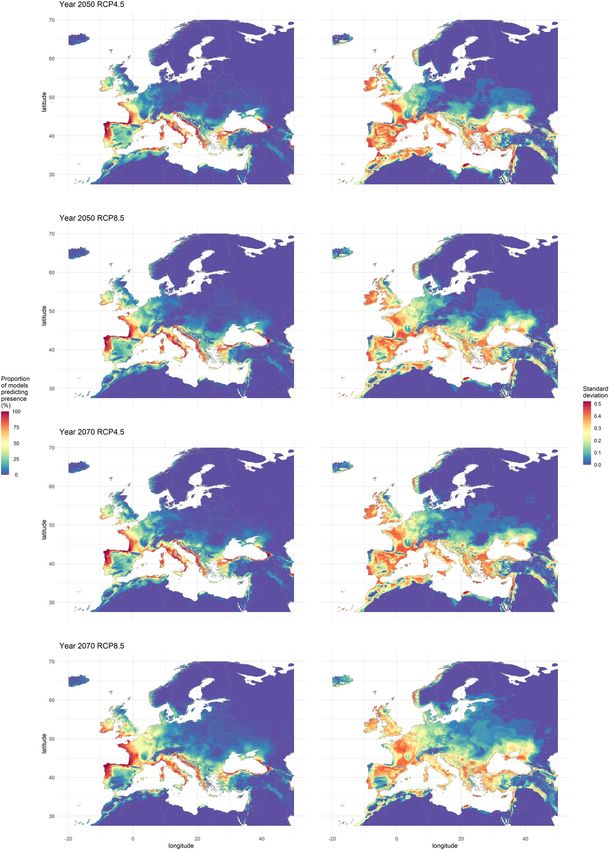
around 0.1% was consensually predicted as suitable (Fig. 3). Yet, the results for 2070 with RCP8.5 in Europe
Scientific Reports | (2021) 11:1339 | https://doi.org/10.1038/s41598-020-80157-9 4
Vol:.(1234567890)www.nature.com/scientificreports/
Figure 2. Consensus map showing habitat suitability for Xylosandrus compactus under current climate
conditions. This consensus map was computed by averaging binary maps and represents the percentage of
models predicting each pixel as suitable. The black square represents the limits of the focal area. The map was
generated using R 4.0.0 (https://cran.r-project.org/).
stood out with 45% of the world unanimously predicted as non-suitable and only 0.02% of the area unanimously
predicted as suitable. Around 60% of the world and 70% of the focal area reached a high agreement. For the 4
RCPs, we observed a progression of the habitat suitability towards North and Northeast between the current cli-
mate and the projections for 2050 in the focal area, where the consensus map shows that the majority of Western
Europe would become suitable. However, the suitability was predicted to decrease in Southwestern Spain, along
the coasts of Morocco and Algeria, and in the easternmost parts of the Mediterranean (Israel, Turkey, Greece).
We observed the same trends between 2050 and 2070 for the RCP4.5, 6.0 and 8.5. Over the same period, we
observed the opposite trend for the RCP2.6, with a regression of the habitat suitability in the North and North-
eastern areas and a progression in North Africa and East of the Mediterranean Sea. Outside the focal area, we
observed an increase of the habitat suitability between 2050 and 2070 in Northern USA, around Uruguay, in
central Africa, in Oceania and some regions of Asia. Conversely, we observed a regression around Venezuela,
Central America and some areas in the USA.
The standard deviation of predicted habitat suitability is given in Fig. 3 and in Supplementary material, Fig.
S3. These maps highlight the areas where models’ projections diverge, showing low values near the coastline,
where most models predict on high suitability, and in the North-east Europe, where most models agree predict
low suitability.
We observed the same type of predictions when comparing the GCM maps between 2050 and 2070 for each
RCP. This is also true for most comparisons between RCPs amongst each predicted year. However, this was not
true when comparing the predictions between GCMs, which generated divergent results. Figure 4 highlights the
variability of the model outputs according to GCMs for a given scenario. While maps A and D both displayed
under average suitability in Western Europe and the Balkans and over average values near Gibraltar, maps B and
C displayed symmetrical results. On the same principle, we were able to group GCMs according to their predic-
tions. For the year 2050 and RCP2.6, the maps for the GCMs HD and HE displayed above-average suitability
over the focal area. Conversely, the GCMs CC, GS and MG predicted a lower than average suitability for most of
the focal area but South-eastern Spain and Northern Africa. The other GCMs patterns were less structured (IP,
MI and MR) or close to the average predictions (BC, NO, MC). At the worldwide scale, NO and MG predicted
above-average suitability in Eastern China, South-eastern USA and Northern South America until Paraguay and
North America. On the contrary, HE, MI and MR predicted below average suitability for these regions.
Discussion
Several pest risk analyses have been performed on species of the Xylosandrus genus in Europe in the last decade
(UK53, France54, Slovenia55). However, while they assessed the species’ ability to enter, establish and spread in the
area of interest, the establishment part mostly focused on the presence of host species and lacked information
about climate suitability. Our study provides the first attempt to model the potential distribution of Xylosandrus
compactus and X. crassiusculus, two invasive species whose range has been increasing ceaselessly during the last
century. Both species have similar ecology and invasion history, suggesting that their potential distribution could
be quite similar and thus that their respective models would produce analogous outputs. However, surprisingly,
no model created for X. crassiusculus matched our criteria.
Failure to model Xylosandrus crassiusculus’ species distribution. The failure in appropriately
modelling X. crassiusculus’ potential distribution could be explained by several factors, mutually compatible.
Scientific Reports | (2021) 11:1339 | https://doi.org/10.1038/s41598-020-80157-9 5
Vol.:(0123456789)www.nature.com/scientificreports/
Figure 3. On the left side, consensus maps showing habitat suitability for Xylosandrus compactus under future
climate for 2 greenhouse gases concentration scenarios (RCP4.5 and 8.5) and for 2 years (2050 and 2070).
These consensus maps were computed by averaging presence–absence maps and represent the percentage of
models predicting each pixel as suitable. On the right side, maps representing the standard deviation of their
left counterpart where the higher values the lower the agreement between models’ predictions. The maps were
generated using R 4.0.0 (https://cran.r-project.org/).
Scientific Reports | (2021) 11:1339 | https://doi.org/10.1038/s41598-020-80157-9 6
Vol:.(1234567890)www.nature.com/scientificreports/
Figure 4. Illustration of the variability between the GCMs used to create consensus maps using centered
and standardised maps. These display a negative value when the GCM considered predicts a lower suitability
than the average of all GCMs and a positive value otherwise. A and B correspond to two GCMs (MG and MI
respectively) used to compute the RCP2.6 maps for the year 2050, C and D represent two GCM (HD and MG
respectively) used to compute the RCP8.5 for the year 2070. The maps were generated using R 4.0.0 (https://
cran.r-project.org/).
Our first hypothesis is that we may have overlooked crucial information when performing SDM on X. cras-
siusculus. According to the literature, X. crassiusculus is genetically structured and could be divided into two or
more differentiated clades, corresponding to potential cryptic d iversity56,57. It has been shown that integrating
phylogeographical information into SDM can alter the results when performing SDM on different clades of a
species58,59. Yet, as genetic studies concerning X. crassiusculus in different regions of the world did not rely on
similar molecular markers, it is not possible at present to determine which clade occurs in a given region. We
thus tested the SDM approach at the species level, i.e. all occurrences were used to calibrate the model. In doing
so, we possibly grouped clades with potentially different ecological features, hence building models with weak
predictive power. To counter this problem, we are currently working on a comprehensive genetic analysis of X.
crassiusculus worldwide, to get a better insight about its genetic structure and assign a clade to each locality. This
would then allow us to perform a SDM for each clade separately.
Another hypothesis is that SDM relies on several assumptions that can easily be violated when working on
expanding invasive species. One is that species are supposed to be at equilibrium, which means that they should
be present in all suitable areas60. However, we know that X. crassiusculus is still expanding. Moreover, even though
we reached more than 300 occurrence records, we might have under-sampled the native area, which could pre-
vent us from inferring X. crassiusculus’ realised niche. Indeed, particular populations can sometimes evolve to
face a harsher environment, and thus be preadapted to certain conditions, which ease further i nvasion61. Failing
to include such peculiar populations might affect SDM outputs, although it is difficult to evaluate the magnitude
of such effect. A last possible explanation for SDM failure could be related to variable selection, but this latter
possibility appears very unlikely as we followed the same procedure as for X. compactus and created models with
126 variable datasets made of 11 environmental variables.
Scientific Reports | (2021) 11:1339 | https://doi.org/10.1038/s41598-020-80157-9 7
Vol.:(0123456789)www.nature.com/scientificreports/
Potential distribution of X. compactus under current climate. Correlative SDM uses relationships
between environmental predictors and species’ occurrences to predict its potential distribution. Therefore,
unreliable information regarding X. compactus’ distribution such as countries for which exact occurrence data
were not mentioned, or localities where the species was detected but was not proved to have settled, had to be
removed from datasets. Despite these precautions, our model successfully spotted suitable areas that were not
initially included in the occurrence dataset (e.g., in Central Africa and Oceania) for X. compactus. Similarly, the
models predicted the Greek province of Peloponnese and the Balearic Island Mallorca, where it was reported as
established after we stopped gathering occurrence data30,31, which suggests that the models have good predictive
power. According to our model, X. compactus’ distribution in America could expand to Chile and Argentina, all
Central America and the Western coast of North America. In the focal area, most of the Mediterranean coasts
and the westernmost parts of the UK are predicted as suitable. Besides Northwest Australia, almost all Oceania
and South East Asia is expected to be suitable. This suggests that even in its native area in Asia, X. compactus
might colonise new areas or islands where it is not present yet. Even though X. compactus has proven to be very
adaptable, invading different climatic regions in the last century, our models unanimously predicted more than
50% of the world’s area as not suitable. Most of these areas are considered arid or semi-arid62 whether hot (e.g.
Sahara or Arabian Peninsula) or cold (e.g. Canada or Andean Mountains). Little is known about the critical
thermal minimum and maximum limits in species of the Xylosandrus genus, which could be used as thresholds
constraining X. compactus’ distribution. Gugliozzo et al.63 fitted a linear relationship between mortality and
minimum temperature and found a 40% mortality in overwintering adults when the minimum temperatures
decreased to 5 °C. The study did not record temperature under 5 °C, far from the lower lethal temperature of
10 °C observed for Xyleborus glabratus, another ambrosia beetle64. Some Xylosandrus species, including X. com-
pactus, showed an absence of flight activity under 20 °C65,66, a temperature threshold which may act as another
constraining parameter. X. compactus’ distribution is expected to shift with climate change as precipitations and
temperature patterns are modified.
Potential distribution of X. compactus under future climate conditions. The direction and mag-
nitude of a range shift depend on how climate change will affect the environmental parameters that constrain the
species’ distribution67. Being generalist and carrying its symbiotic fungi to feed on, X. compactus’ distribution is
expected to be mostly dependent on temperature and humidity. However, X. compactus lives most of its life in
galleries, where wood acts as a buffer, protecting individuals from ambient air temperature and extreme events64.
The uncertainties of predictions were higher when dealing with future conditions compared to the consensus
obtained under the current climate. Indeed, apart from Central Africa, the values observed on the consensus
maps are usually lower. Whereas the areas predicted as suitable by at least some models stretches polewards in
the Northern hemisphere, the predicted suitability in the Southern hemisphere is less consistent, decreasing over
time in some places but not in others. In the focal area, the habitat suitability is predicted to increase going North
and Northeast, reaching Central Europe, the Balkans and the Black Sea. However, outside the focal area, no new
country is projected to become suitable between now and 2050 or 2070.
Even though some GCMs can make close predictions for the environmental parameters’ value in the future, it
is necessary to use several of them when predicting species’ potential distribution. Indeed, when using general-
purpose machine learning methods such as MaxEnt, which relies on complex relations between the predictors to
assess if areas are suitable or not, even small differences could lead to unpredictable and substantial differences in
the final p redictions12. Moreover, performing models over a range of GCMs and RCPs provide decision-makers
more reliable information regarding species’ potential distribution under future climate, notably regarding the
areas predicted as unsuitable. On this point, our study is remarkable as it uses an exceptionally high number
of GCMs, sometimes predicting divergent if not symmetrical results, and 4 RCPs, aimed at representing four
different potential futures. Indeed, in their review, Porfirio et al.12 found that 40% of the studies (out of 163)
used 2 or more GCMs, with only 7 using more than 10 GCMs, all being focused on methodology and not on
conservation issues.
Risk prevention and invasion management. In addition to altering ambrosia beetles’ distribution, cli-
mate change might increase the damage they cause68. On the one hand, temperature changes could facilitate
their survival and development and thus significantly modify their population dynamics. On the other hand,
changes in precipitations pattern would impact tree by prompting stress-induced ethanol emissions, which
might increase their susceptibility to ambrosia b eetles69,70. While ambrosia beetles have been eradicated when
established in very localised areas71, this strategy is most of the time unsuccessful. Indeed, they live most of their
lives inside galleries where they are protected from pesticides, parasitoids and predators. Moreover, these eco-
logical characteristics make them difficult to detect, which prevent efficient eradication strategies. Even if cutting
and destroying infested trees can reduce population density, it is not applicable with high population densities
or already widespread species.
The most cost effective management strategy is to prevent species’ invasion in the first place. Wood trans-
portation is a major introduction pathway for bark and ambrosia b eetles68, allowing them to disperse over long
distances passively. However, even if phytosanitary measures are in place to prevent involuntarily transporting
species (e.g. heat treatment or fumigation of the wood), they are not sufficient to ensure that no specimen reaches
its destination alive. Moreover, bark and ambrosia beetles are also known to travel in living plants, which do not
comply with the same regulations. To limit species’ invasion through wood and living plant transportation, a
strengthening of the regulation might be necessary. However, resources are limited, so it is essential to prioritise
areas to survey. For monophagous or oligophagous invasive species, the invasion pathways and currently suitable
areas can be determined using host species transportation and distribution. However, both X. compactus and
Scientific Reports | (2021) 11:1339 | https://doi.org/10.1038/s41598-020-80157-9 8
Vol:.(1234567890)www.nature.com/scientificreports/
X. crassiusculus are known to have a broad range of h osts31,72, and more are added to the list as they invade new
regions73. Hence, managers should not rely on pre-existing host lists as a way to consider an area as unsuitable.
Our result relies on environmental parameters to show which areas are suitable for X. compactus. This could
significantly improve the future pest risk analyses, in addition to being a helpful tool for decision-makers when
making policies about trapping for early detection of X. compactus. Indeed, our results show that some areas
are still free of X. compactus even though they are predicted as suitable, today or in the future. We suggest that
such areas should be prioritised for early detection strategy, while efforts could be partially relaxed in regions
unanimously predicted as unsuitable in the present study.
Received: 24 July 2020; Accepted: 14 December 2020
References
1. Lenzner, B. et al. A framework for global twenty-first century scenarios and models of biological invasions. Bioscience 69, 697–710.
https://doi.org/10.1093/biosci/biz070 (2019).
2. Sun, Y. et al. Rapid increase in the risk of extreme summer heat in Eastern China. Nat. Clim. Change 4, 1082–1085. https://doi.
org/10.1038/nclimate2410 (2014).
3. van der Geest, K. et al. in Loss and Damage from Climate Change Climate Risk Management, Policy and Governance (eds Mechler
R. et al.) 221–236 (2018).
4. Sage, R. F. Global change biodiversity: A primer. Glob. Change Biol. 26, 3–30. https://doi.org/10.1111/gcb.14893 (2020).
5. Nunez-Mir, G. C., Guo, Q., Rejmanek, M., Iannone, B. V. III. & Fei, S. Predicting invasiveness of exotic woody species using a
traits-absed framework. Ecol. Lett. 100, e02797. https://doi.org/10.1002/ecy.2797 (2019).
6. Zeng, J. et al. Global warming modifies long-distance migration of an agricultural insect pest. J. Pest. Sci. 93, 569–581. https://doi.
org/10.1007/s10340-019-01187-5 (2020).
7. Gippet, J. M. W., Liebhold, A. M., Fenn-Moltu, G. & Bertelsmeier, C. Human-mediated dispersal in insects. Curr. Opin. Insect Sci.
35, 96–102. https://doi.org/10.1016/j.cois.2019.07.005 (2019).
8. Cassey, P., Delean, S., Lockwood, J. L., Sadowski, J. S. & Blackburn, T. M. Dissecting the null model for biological invasions: A
meta-analysis of the propagule pressure effect. PLoS Biol 16, e2005987. https://doi.org/10.1371/journal.pbio.2005987 (2018).
9. Reaser, J. K. et al. The early detection of and rapid response (EDRR) to invasive species: A conceptual framework and federal
capacities assessment. Biol. Invas. 22, 1–19. https://doi.org/10.1007/s10530-019-02156-w (2019).
10. Guisan, A., Thuiller, W. & Zimmermann, N. E. Habitat Suitability and Distribution Models (Cambridge University Press, Cambridge,
2017).
11. Soberon, J. & Townsend Peterson, A. Interpretation of models of fundamental ecological niches and species’ distributional areas.
Biodiv. Inform. 2, 1–10. https://doi.org/10.17161/bi.v2i0.4 (2005).
12. Porfirio, L. L. et al. Improving the use of species distribution models in conservation planning and management under climate
change. PLoS One 9, e113749. https://doi.org/10.1371/journal.pone.0113749 (2014).
13. IPCC. Synthesis Report. Contribution of Working Groups I, II and III to the Fifth Assessment Report of the Intergovernmental Panel
on Climate Change 151 (IPCC, Geneva, 2014).
14. Beaumont, L. J., Hughes, L. & Pitman, A. J. Why is the choice of future climate scenarios for species distribution modelling impor-
tant?. Ecol. Lett. 11, 1135–1146. https://doi.org/10.1111/j.1461-0248.2008.01231.x (2008).
15. Buisson, L., Thuiller, W., Casajus, N., Lek, S. & Grenouillet, G. Uncertainty in ensemble forecasting of species distribution. Glob.
Change Biol. 16, 1145–1157. https://doi.org/10.1111/j.1365-2486.2009.02000.x (2010).
16. Faccoli, M. et al. A first worldwide multispecies survey of invasive Mediterranean pine bark beetles (Coleoptera: Curculionidae,
Scolytinae). Biol. Invas. 22, 1785–1799. https://doi.org/10.1007/s10530-020-02219-3 (2020).
17. Kirkendall, L. R. & Faccoli, M. Bark beetles and pinhole borers (Curculionidae, Scolytinae, Platypodinae) alien to Europe. Zookeys
56, 227–251. https://doi.org/10.3897/zookeys.56.529 (2010).
18. Raffa, K. F., Grégoire, J.-C. & StaffanLindgren, B. Economics and politics of bark beetles. In Bark Beetles. Biology and Ecology of
Native and Invasive Species (eds Fernando, E. V. & Richard, W. H.) 585–614 (Elsevier, New York, 2015).
19. Ngoan, N. D., Wilkinson, R. C., Short, D. E., Moses, C. S. & Mangold, J. R. Biology of an introduced ambrosia beetle, Xylosandrus
compactus, in Florida. Ann. Entomol. Soc. Am. 69, 872–876. https://doi.org/10.1093/aesa/69.5.872 (1976).
20. Hara, A. H. & Beardsley, J. W. Jr. The biology of the black twig borer, Xylosandrus compactus (Eichhoff), in Hawaii. Proc. Hawaiian
Entomol. Soc. 13, 55–70 (1979).
21. Wood, S. L. New american bark beetles (Coleoptera: Scolytidae) with two recently introduced species. Great Basin Nat. 40, 353–358
(1980).
22. Samuelson, G. A. A synopsis of Hawaiian Xyleborini (Coleoptera: Scolytidae). Pac. Insects 23, 50–92 (1981).
23. Anderson, D. M. First record of Xyleborus semiopacus in the continental United States (Coleoptera, Scolytidae). Cooper. Econ.
Insect Rep. 24, 863–864 (1974).
24. Kirkendall, L. Invasive bark beetles (Coleoptera, Curculionidae, Scolytinae) in Chile and Argentina, including two species new for
South America, and the correct identity of the Orthotomicus species in Chile and Argentina. Diversity https://doi.org/10.3390/
d10020040 (2018).
25. Pennachio, F., Roversi, P. F., Francardi, V. & Gatti, E. Xylosandrus crassiusculus (Motschulsky) a bark beetle new to Europe (Coleop-
tera Scolytidae). Redia 86, 77–80 (2003).
26. Garonna, A. P., Dole, S. A., Saracino, A., Mazzoleni, S. & Cristinzio, G. First record of the black twig borer Xylosandrus compactus
(Eichhoff) (Coleoptera: Curculionidae, Scolytinae) from Europe. Zootaxa 3251, 64–68. https://doi.org/10.11646/zootaxa.3251.1.5
(2012).
27. Roques, A. et al. Les scolytes exotiques: Une menace pour le maquis. Phytoma 727, 16–20 (2019).
28. Gallego, D., Lencina, J. L., Mas, H., Cevero, J. & Faccoli, M. First record of the granulate ambrosia beetle, Xylosandrus crassius-
culus (Coleoptera: Curculionidae, Scolytinae), in the Iberian Peninsula. Zootaxa 4273, 431–434. https://doi.org/10.11646/zoota
xa.4273.3.7 (2017).
29. Kavčič, A. First record of the Asian ambrosia beetle, Xylosandrus crassiusculus (Motschulsky) (Coleoptera: Curculionidae, Scoly-
tinae), Slovenia. Zootaxa 4483, 191–193. https://doi.org/10.11646/zootaxa.4483.1.9 (2018).
30. Spanou, K. et al. in 18th Panhellenic Entomological Congress (Komotini, 2019).
31. Leza, M. A. R. et al. First record of the black twig borer, Xylosandrus compactus (Coleoptera: Curculionidae, Scolytinae) in Spain.
Zootaxa 4767, 345–350. https://doi.org/10.11646/zootaxa.4767.2.9 (2020).
32. Greco, E. B. & Wright, M. G. Ecology, biology, and management of Xylosandrus compactus (Coleoptera: Curculionidae: Scolytinae)
with emphasis on coffee in Hawaii. J. Integrat. Pest Manag. 6, 1–8. https://doi.org/10.1093/jipm/pmv007 (2015).
Scientific Reports | (2021) 11:1339 | https://doi.org/10.1038/s41598-020-80157-9 9
Vol.:(0123456789)www.nature.com/scientificreports/
33. Kirkendall, L. R., Dal Cortivo, M. & Gatti, E. First record of the ambrosia beetle, Monarthrum mali (Curculionidae, Scolytinae)
in Europe. J. Pest. Sci. 81, 175–178. https://doi.org/10.1007/s10340-008-0196-y (2008).
34. Jordal, B. H., Beaver, R. A. & Kirkendall, L. R. Breaking taboos in the tropics: Incest promotes colonization by wood-boring beetles.
Glob. Ecol. Biogeogr. 10, 345–357. https://doi.org/10.1046/j.1466-822X.2001.00242.x (2001).
35. Douglas, H. et al. New Curculionoidea (Coleoptera) records for Canada. Zookeys 309, 13–48. https://doi.org/10.3897/zooke
ys.309.4667 (2013).
36. EPPO. EPPO Technical Document No. 1081, Study on the risk of bark and ambrosia beetles associated with imported non-
coniferous wood. (2020).
37. Guiot, J. & Cramer, W. Climate change: The 2015 Paris agreement thresholds and Mediterranean basin ecosystems. Science 354,
465–468. https://doi.org/10.1126/science.aah5015 (2016).
38. Fick, S. E. & Hijmans, R. J. WorldClim 2: New 1km spatial resolution climate surfaces for global land areas. Int. J. Climatol. 37,
4302–4315. https://doi.org/10.1002/joc.5086 (2017).
39. Radosavljevic, A., Anderson, R. P. & Araújo, M. Making better Maxent models of species distributions: Complexity, overfitting
and evaluation. J. Biogeogr. 41, 629–643. https://doi.org/10.1111/jbi.12227 (2014).
40. Beaumont, L. J. et al. Which species distribution models are more (or less) likely to project broad-scale, climate-induced shifts in
species ranges?. Ecol. Model. 342, 135–146. https://doi.org/10.1016/j.ecolmodel.2016.10.004 (2016).
41. Phillips, S. J., Anderson, R. P. & Schapire, R. E. Maximum entropy modeling of species geographic distributions. Ecol. Model. 190,
231–259. https://doi.org/10.1016/j.ecolmodel.2005.03.026 (2006).
42. Godefroid, M., Meurisse, N., Groenen, F., Kerdelhué, C. & Rossi, J. P. Current and future distribution of the invasive oak proces-
sionary moth. Biol. Invas. 22, 523–534. https://doi.org/10.1007/s10530-019-02108-4 (2019).
43. Qiao, H., Soberón, J., Peterson, A. T. & Kriticos, D. No silver bullets in correlative ecological niche modelling: Insights from testing
among many potential algorithms for niche estimation. Methods Ecol. Evol. 6, 1126–1136. https: //doi.org/10.1111/2041-210x.12397
(2015).
44. Muscarella, R. et al. ENMeval: An R package for conducting spatially independent evaluations and estimating optimal model
complexity for ecological niche models. Methods Ecol. Evol. 5, 1198–1205. https://doi.org/10.1111/2041-210X.12261 (2014).
45. Gettelman, A. & Rood, R. B. A Users Guide to Earth System Models Earth Systems Data and Models 282 (Springer, Berlin, 2016).
46. R Core Team. R: A Language and Environment for Statistical Computing (R Foundation for Statistical Computing, Vienna, 2018).
47. Hijmans, R. J., Phillips, S., Leathwick, J. & Elith, J. Dismo: Species Distribution Modeling. R package version 1.1-4. (2017).
48. Thuiller, W., Georges, D., Engler, R. & Breiner, F. biomod2: Ensemble platform for species distribution modeling. R package version
3.3-7.1. (2019).
49. Wilke, C. O. cowplot: Streamlined plot theme and plot annotations for ’ggplot2’. R package version 0.9.4. (2019).
50. Wickham, H. ggplot2: Elegant Graphics for Data Analysis (Springer, New York, 2016).
51. South, A. rnaturalearth: World Map Data from Natural Earth. R package version 0.1.0. (2017).
52. Hijmans, R. J. raster: Geographic Data Analysis and Modeling. R package version 3.0-7. (2019).
53. Department for Environment Food and Rural Affairs. Rapid pest risk analysis for Xylosandrus crassisuculus. 30 (2015).
54. ANSES. Évaluation du risque simplifiée sur Xylosandrus compactus (Eichhoff) identifié en France métropolitaine. (2017).
55. Kavčič, A. & de Groot, M. Pest risk analysis for the Asian Ambrosia Beetle (Xylosandrus crassiusculus (Motschulsky, 1866)). (Slo-
venian Forestry Institute, 2017).
56. Storer, C., Payton, A., McDaniel, S., Jordal, B. & Hulcr, J. Cryptic genetic variation in an inbreeding and cosmopolitan pest,
Xylosandrus crassiusculus, revealed using ddRADseq. Ecol. Evol. 7, 10974–10986. https://doi.org/10.1002/ece3.3625 (2017).
57. Ito, M. & Kajimura, H. Phylogeography of an ambrosia beetle, Xylosandrus crassiusculus (Motschulsky) (Coleoptera: Curculionidae:
Scolytinae), Japan. Appl. Entomol. Zool. 44, 549–559. https://doi.org/10.1303/aez.2009.549 (2009).
58. Godefroid, M., Rasplus, J.-Y. & Rossi, J.-P. Is phylogeography helpful for invasive species risk assessment? The case study of the
bark beetle genus Dendroctonus. Ecography 39, 1197–1209. https://doi.org/10.1111/ecog.01474 (2016).
59. Godefroid, M., Cruaud, A., Rossi, J. P. & Rasplus, J. Y. Assessing the risk of invasion by Tephritid fruit flies: Intraspecific divergence
matters. PLoS One 10, e0135209. https://doi.org/10.1371/journal.pone.0135209 (2015).
60. Gallien, L., Douzet, R., Pratte, S., Zimmermann, N. E. & Thuiller, W. Invasive species distribution models—how violating the equi-
librium assumption can create new insights. Glob. Ecol. Biogeogr. 21, 1126–1136. https://doi.org/10.1111/j.1466-8238.2012.00768
.x (2012).
61. Rey, O. et al. Where do adaptive shifts occur during invasion? A multidisciplinary approach to unravelling cold adaptation in a
tropical ant species invading the Mediterranean area. Ecol. Lett. 15, 1266–1275. https://doi.org/10.1111/j.1461-0248.2012.01849
.x (2012).
62. Ma, Z. & Yang, Q. (2017) Global patterns of aridity trends and time regimes in transition. In Aridity Trend in Northern China (eds
Congbin, F. & Huiting, M.) 67–90 (World Scientific Publishing, Singapore, 2017).
63. Gugliuzzo, A. et al. Seasonal changes in population structure of the ambrosia beetle Xylosandrus compactus and its associated fungi
in a southern Mediterranean environment. PLoS One 15, e0239011. https://doi.org/10.1371/journal.pone.0239011 (2020).
64. Formby, J. P. et al. Cold tolerance and invasive potential of the redbay ambrosia beetle (Xyleborus glabratus) in the eastern United
States. Biol. Invas. 20, 995–1007. https://doi.org/10.1007/s10530-017-1606-y (2017).
65. Reding, M. E., Ranger, C. M., Oliver, J. B. & Schultz, P. B. Monitoring attack and flight activity of Xylosandrus spp. (Coleoptera:
Curculionidae: Scolytinae): The influence of temperature on activity. Hortic. Entomol. 106, 1780–1787. https://doi.org/10.1603/
ec13134 (2013).
66. Gugliuzzo, A., Criscione, G., Siscaro, G., Russo, A. & Tropea Garzia, G. First data on the flight activity and distribution of the
ambrosia beetle Xylosandrus compactus (Eichhoff) on carob trees in Sicily. EPPO Bull. 49, 340–351. https://doi.org/10.1111/
epp.12564(2019).
67. Williams, J. E. & Blois, J. L. Range shifts in response to past and future climate change: Can climate velocities and species’ dispersal
capabilities explain variation in mammalian range shifts?. J. Biogeogr. 45, 2175–2189. https://doi.org/10.1111/jbi.13395 (2018).
68. Hlásny, T. et al. Living with Bark Beetles: Impacts, Outlook and Management Options 52 (European Forest Institute, Joensuu, 2019).
69. Ranger, C. M., Schultz, P. B., Frank, S. D., Chong, J. H. & Reding, M. E. Non-native ambrosia beetles as opportunistic exploiters
of living but weakened trees. PLoS One 10, e0131496. https://doi.org/10.1371/journal.pone.0131496 (2015).
70. Ranger, C. M., Reding, M. E., Schultz, P. B. & Oliver, J. B. Influence of flood-stress on ambrosia beetle host-selection and implica-
tions for their management in a changing climate. Agric. For. Entomol. 15, 56–64. https://doi.org/10.1111/j.1461-9563.2012.00591
.x (2013).
71. LaBonte, J. R. in USDA Research Forum on Invasive Species. 41–43.
72. Castrillo, L. A., Griggs, M. H., Ranger, C. M., Reding, M. E. & Vandenberg, J. D. Virulence of commercial strains of Beauveria
bassiana and Metarhizium brunneum (Ascomycota: Hypocreales) against adult Xylosandrus germanus (Coleoptera: Curculionidae)
and impact on brood. Biol. Control 58, 121–126. https://doi.org/10.1016/j.biocontrol.2011.04.010 (2011).
73. Horn, S. & Horn, G. N. New host record for the asian ambrosia beetle, Xylosandrus crassiusculus (Motschulsky) (Coleoptera:
Curculionidae). J. Entomol. Sci. 41, 90–91. https://doi.org/10.18474/0749-8004-41.1.90 (2006).
74. Wu, T. et al. An overview of BCC climate system model development and application for climate change studies. J. Meteorol. Res.
28, 34–56. https://doi.org/10.1007/s13351-014-3041-7 (2013).
Scientific Reports | (2021) 11:1339 | https://doi.org/10.1038/s41598-020-80157-9 10
Vol:.(1234567890)www.nature.com/scientificreports/
75. Gent, P. R. et al. The community climate system model version 4. J. Clim. 24, 4973–4991. https://doi.org/10.1175/2011jcli4083.1
(2011).
76. Schmidt, G. A. et al. Configuration and assessment of the GISS ModelE2 contributions to the CMIP5 archive. J. Adv. Model. Earth
Syst. 6, 141–184. https://doi.org/10.1002/2013ms000265 (2014).
77. Collins, W. J. et al. Development and evaluation of an Earth-System model—HadGEM2. Geosci. Model Dev. 4, 1051–1075. https
://doi.org/10.5194/gmd-4-1051-2011 (2011).
78. Dufresne, J. L. et al. Climate change projections using the IPSL-CM5 Earth System Model: From CMIP3 to CMIP5. Clim. Dyn.
40, 2123–2165. https://doi.org/10.1007/s00382-012-1636-1 (2013).
79. Watanabe, M. et al. Improved climate simulation by MIROC5: Mean states, variability, and climate sensitivity. J. Clim. 23, 6312–
6335. https://doi.org/10.1175/2010jcli3679.1 (2010).
80. Yukimoto, S. et al. A new global climate model of the Meteorological Research Institute: MRI-CGCM3. J. Meteorol. Soc. Jpn 90A,
23–64. https://doi.org/10.2151/jmsj.2012-A02 (2012).
81. Watanabe, S. et al. MIROC-ESM 2010: Model description and basic results of CMIP5-20c3m experiments. Geosci. Model Dev. 4,
845–872. https://doi.org/10.5194/gmd-4-845-2011 (2011).
82. Bentsen, M. et al. The Norwegian earth system model, NorESM1-M—Part 1: Description and basic evaluation of the physical
climate. Geosci. Model Dev. 6, 687–720. https://doi.org/10.5194/gmd-6-687-2013 (2013).
Acknowledgements
We would like to thank Giovanna Tropea, Jared Bernard, Andrew Johnson and You Li for sharing their occur-
rence data with us. This work was supported by the LIFE project SAMFIX (SAving Mediterranean Forests from
Invasions of Xylosandrus beetles and associated pathogenic fungi, LIFE17 NAT/IT/000609, https://www.lifes
amfix.eu/) which received funding from the European Union’s LIFE Nature and Biodiversity programme.
Author contributions
C.K., M.A.A.R. and J.P.R. designed the study. T.U. collected the data. T.U. and J.P.R. performed the analysis and
made the figures. T.U. wrote the original draft of the manuscript. All authors reviewed, edited and approved the
final version of the manuscript.
Competing interests
The authors declare no competing interests.
Additional information
Supplementary Information The online version contains supplementary material available at https://doi.
org/10.1038/s41598-020-80157-9.
Correspondence and requests for materials should be addressed to T.U.
Reprints and permissions information is available at www.nature.com/reprints.
Publisher’s note Springer Nature remains neutral with regard to jurisdictional claims in published maps and
institutional affiliations.
Open Access This article is licensed under a Creative Commons Attribution 4.0 International
License, which permits use, sharing, adaptation, distribution and reproduction in any medium or
format, as long as you give appropriate credit to the original author(s) and the source, provide a link to the
Creative Commons licence, and indicate if changes were made. The images or other third party material in this
article are included in the article’s Creative Commons licence, unless indicated otherwise in a credit line to the
material. If material is not included in the article’s Creative Commons licence and your intended use is not
permitted by statutory regulation or exceeds the permitted use, you will need to obtain permission directly from
the copyright holder. To view a copy of this licence, visit http://creativecommons.org/licenses/by/4.0/.
© The Author(s) 2021
Scientific Reports | (2021) 11:1339 | https://doi.org/10.1038/s41598-020-80157-9 11
Vol.:(0123456789)You can also read