Alan Turing and the Other Theory of Computation (expanded)
←
→
Page content transcription
If your browser does not render page correctly, please read the page content below
Alan Turing and the Other Theory of
                  Computation (expanded)*

                            Lenore Blum
        Computer Science Department, Carnegie Mellon University

Abstract. We recognize Alan Turing’s work in the foundations of numerical com-
putation (in particular, his 1948 paper “Rounding-Off Errors in Matrix Processes”), its
influence in modern complexity theory, and how it helps provide a unifying concept
for the two major traditions of the theory of computation.

1       Introduction
The two major traditions of the theory of computation, each staking claim to simi-
lar motivations and aspirations, have for the most part run a parallel non-intersecting
course. On one hand, we have the tradition arising from logic and computer science ad-
dressing problems with more recent origins, using tools of combinatorics and discrete
mathematics. On the other hand, we have numerical analysis and scientific compu-
tation emanating from the classical tradition of equation solving and the continuous
mathematics of calculus. Both traditions are motivated by a desire to understand the
essence of computation, of algorithm; both aspire to discover useful, even profound,
consequences.
While the logic and computer science communities are keenly aware of Alan Turing’s
seminal role in the former (discrete) tradition of the theory of computation, most
remain unaware of Alan Turing’s role in the latter (continuous) tradition, this notwith-
standing the many references to Turing in the modern numerical analysis/computational
    *
    This paper amplifies a shorter version to appear in The Selected Works of A.M. Turing: His Work and
Impact, Elsevier [Blu12] and follows the perspective presented in “Computing over the Reals: Where
Turing Meets Newton,” [Blu04].

                                                  1
mathematics literature, e.g., [Bür10, Hig02, Kah66, TB97, Wil71]. These references
are not to recursive/computable analysis (suggested in Turing’s seminal 1936 paper),
usually cited by logicians and computer scientists, but rather to the fundamental role
that the notion of “condition” (introduced in Turing’s seminal 1948 paper) plays in real
computation and complexity.
In 1948, in the first issue of the Quarterly Journal of Mechanics and Applied Mathematics,
sandwiched between a paper on “Use of Relaxation Methods and Fourier Transforms”
and “The Position of the Shock-Wave in Certain Aerodynamic Problems,” appears the
article “Rounding-Off Errors in Matrix Processes.” This paper introduces the notion
of the condition number of a matrix, the chief factor limiting the accuracy in solving
linear systems, a notion fundamental to numerical computation and analysis, and a
notion with implications for complexity theory today. This paper was written by Alan
Turing [Tur48].
After the war, with the anticipation of a programmable digital computing device on the
horizon, it was of great interest to understand the comparative merits of competing
computational “processes” and how accurate such processes would be in the face of
inevitable round-off errors. Solving linear systems is basic. Thus for Turing (as it was
for John von Neumann [vNG47]), examining methods of solution with regard to the
ensuing round-off errors presented a compelling intellectual challenge.1
1
It is clear that Turing and von Neumann were working on similar problems, for similar reasons,
2In 1945, Turing had submitted an 86 page proposal to the British National Physical
Laboratory (NPL) for the Automatic Computing Engine (ACE), an automatic electronic
digital computer with internal program storage [Tur45]. This was to be an incarnation of
the universal machine envisioned by his theoretical construct in “Computable Num-
bers” [Tur36], blurring the boundary between data and program. Thus, and in con-
trast to other proposed “computing machines” at the time, Turing’s computer would
have simplified hardware, with universality emanating from the power of program-
ming.
Turing envisioned an intelligent machine that would learn from its teachers and from
its experience and mistakes, and hence have the ability to create and modify its own
programs. Turing also felt that the most conducive environment for realizing such a
machine was to have mathematicians and engineers working together in close prox-
imity, not in separate domains [Hod92].
Unfortunately, the ACE computer was never to see the light of day;2 a less ambitious
non-universal machine, the PILOT ACE, was constructed after Turing left the NPL
for the University of Manchester in 1948. Although Turing’s central passion during his
time at the NPL was the promised realization of his universal computer, his only pub-
lished paper to come out of this period (1945-1948) was “Round-Off Errors in Matrix
Processes.” 3
“Rounding-Off Errors in Matrix Processes” was by no means an anomaly in Turing’s cre-
ative pursuits. In his 1970 Turing Award Lecture, James Wilkinson writes [Wil71]:
Turing’s international reputation rests mainly on his work on computable
numbers but I like to recall that he was a considerable numerical analyst,
and a good part of his time from 1946 onwards was spent working in this
field...
Wilkinson attributes this interest, and Turing’s decision to go to the NPL after the
war, to the years he spent at Bletchley Park gaining knowledge of electronics and “one
of the happiest times of his life.”
in similar ways at the same time, probably independently. However while Turing acknowledges von
Neumann, as far as I know, von Neumann never cites Turing’s work in this area.
2
An interrelated combination of personalities, rivalries, politics and bureaucracy seems to have been
in play. For an in-depth chronicle of the saga, see Andrew Hodges’ chapter, Mercury Delayed in [Hod92].
3
The paper ends with the cryptic acknowledgement: “published with the permission of the Director
of the National Physical Laboratory.”
3Wilkinson also credits Turing for converting him from a classical to numerical analyst.
From 1946 to 1948, Wilkinson worked for Turing at the NPL on the logical design
of Turing’s proposed Automatic Computing Engine and the problem of programming
basic numerical algorithms:
The period with Turing fired me with so much enthusiasm for the com-
puter project and so heightened my interest in numerical analysis that grad-
ually I abandoned [the idea of returning to Cambridge to take up research
in classical analysis].
Here I would like to recognize Alan Turing’s work in the foundations of numerical
computation. Even more, I would like to indicate how this work has seeded a major
direction in complexity theory of real computation and provides a unifying concept
for the two major traditions in the theory of computation.
2 Rounding-Off Errors in Matrix Processes
This paper contains descriptions of a number of methods for solving sets
of linear simultaneous equations and for inverting matrices, but its main
concern is with the theoretical limits of accuracy that may be obtained in the
application of these methods, due to round-off errors.
So begins Turing’s paper [Tur48]. (Italics are mine, I’ll return to this shortly.)
The basic problem at hand: Given the linear system, Ax = b where A is a real non-
singular n × n matrix and b ∈ Rn. Solve for x ∈ Rn.
Prompted by calculations [FHW48] challenging the arguments by Harold Hotelling
[Hot43] that Gaussian elimination and other direct methods would lead to exponen-
tial round-off errors, Turing introduces quantities not considered earlier to bound the
magnitude of errors, showing that for all “normal” cases, the exponential estimates are
“far too pessimistic.” 4
4
In their 1946 paper, Valentine Bargmann, Deane Montgomery and von Neumann [BMvN63] also
dismissed Gaussian elimination as likely being unstable due to magnification of errors at successive
stages (pp. 430-431) and so turn to iterative methods for analysis. However, in 1947 von Neumann and
Herman Goldstine reassess [vNG47] noting, as does Turing, that it is the computed solution, not the
intermediate computed numbers, which should be the salient object of study. They re-investigated
Gaussian elimination for computing matrix inversion and now give optimistic error bounds similar to
those of Turing, but for the special case of positive definite symmetric matrices. Turing in his paper
notes that von Neumann communicated these results to him at Princeton [during a short visit] in Jan-
4In this paper, Turing introduced the notion of condition number of a matrix making
explicit for the first time a measure that helps formalize the informal notion of ill and
well-conditioned problems.5
3 The Matrix Condition Number: Where Turing Meets
Newton
When we come to make estimates of errors in matrix processes, we shall
find that the chief factor limiting the accuracy that can be obtained is ‘ill-
conditioning’ of the matrices involved [Tur48].
Turing provides an illustrative example:
}
1.4x + 0.9y = 2.7
(8.1)
−0.8x + 1.7y = −1.2
}
−0.786x + 1.709y = −1.173
(8.2)
−0.800x + 1.700y = −1.200
The set of equations (8.1) is fully equivalent to (8.2)6 but clearly if we at-
tempt to solve (8.2) by numerical methods involving rounding-off errors
we are almost certain to get much less accuracy than if we worked with
equations (8.1). ...
We should describe the equations (8.2) as an ill-conditioned set, or, at any
rate, as ill-conditioned compared with (8.1). It is characteristic of ill-conditioned
sets of equations that small percentage errors in the coefficients given may
lead to large percentage errors in the solution.
Turing defines two condition numbers (he calls them N and M), which in essence mea-
sure the intrinsic potential for magnification of errors. He then analyzes various stan-
dard methods for solving linear systems, including Gaussian elimination, and gets error
bounds proportional to his measures of condition. Turing is “also as much interested
uary 1947 before his own proofs were complete.
5
In sections 3 and 4 of his paper, Turing also formulates the LU decomposition of a matrix (actually
the LDU decomposition) and shows that Gaussian elimination computes such a decomposition.
6
The third equation (in the set of four) is the second plus .01 times the first.
5in statistical behaviour of the errors as in the maximum possible values” and presents
probabilistic estimates; he also improves Hotelling’s worst case bound from 4n−1 to
2n−1 [Tur48].
The following widely used (spectral) matrix condition number κ(A), wedged somewhat
between Turing’s condition numbers, is often attributed to Turing, though it is un-
clear who first defined it. (See the discussion in Section 10, Who invented the con-
dition number?) John Todd in his survey [Tod68] is vague on its genesis although he
specifically credits Turing with recognizing “that a condition number should depend
symmetrically on A and A−1 , specifically as a product of their norms.” 7
Definition. Suppose A is a real non-singular n × n matrix. The (spectral) matrix con-
dition number of A is given by
κ (A) = ∥A∥ A−1
where
|Ay|
∥A∥ = sup = sup |Ay|
y̸=0 |y| |y|=1
is the operator (spectral) norm with respect to the Euclidean norm. For singular matri-
ces, define κ (A) = ∞.
This definition can be generalized using other norms. In the case of the Euclidean
norm, κ (A) = σ1 /σn , where σ1 and σ2 are the largest and smallest singular values of
A, respectively. It follows that κ(A) ≥ 1.8
To see how natural a measure this is, consider a slightly more general situation. Let X
and Y be normed vector spaces with associated map φ : X → Y. A measure of the
“condition” of problem instance (φ, x) should indicate how small perturbations of the
input x (the problem data) can alter the output φ(x) (the problem solution).
7
Turing’s N condition number is defined as N(A)N(A−1 ) and the M condition number as
nM(A)M(A−1 ), where N(A) is the Frobenius norm of A and M(A) is the max norm. Turing also de-
fines the spectral norm in this paper, so he could have easily defined the spectral condition number.
8
For the case of computing the inverse of a positive definite symmetric matrix A by Gaussian elimi-
nation, von Neumann and Goldstine [vNG47] give an error estimate bounded by 14.2n2 (λ1 /λ2 )u. Here
λ1 and λ2 are the largest and smallest eigenvalues of A and u is the smallest number recognized by the
machine. For the case of positive definite symmetric matrices, λ1 /λ2 is equal to κ(A). Thus, the spectral
condition number appears implicitly in the von Neumann-Goldstine paper for this case.
6input x
output φ (x )
x +Δx
φ(x+ Δx )
So let ∆x be a small perturbation of input x and ∆φ = φ(x + ∆x) − φ(x). The limit
as ∥∆x∥ goes to zero of the ratio
∥∆φ∥
,
∥∆x∥
or of the relative ratio
∥∆φ∥ / ∥φ(x)∥
∥∆x∥ / ∥x∥
(favored by numerical analysts), will be a measure of the condition of the problem
instance.9 If large, computing the output with small error will require increased preci-
sion, and hence from a computational complexity point of view, increased time/space
resources.
Definition.10 The condition number of problem instance (φ, x) is defined by
∥∆φ∥
b (φ, x) = lim sup
κ ,
δ→0 ∥∆x∥≤δ ∥∆x∥
and the relative condition number by
∥∆x∥ |/ ∥φ(x)∥
κ (φ, x) = lim sup .
δ→0 ∥∆x∥≤δ∥x∥ ∥∆x∥ / ∥x∥
If κ (φ, x) is small, the problem instance is said to be well-conditioned and if large, ill-
conditioned. If κ (φ, x) = ∞, the problem instance is ill-posed.
9
All norms are assumed to be with respect to the relevant spaces.
10
Here I follow the notation in [TB97], a book I highly recommend for background in numerical
linear algebra.
7As Turing envisaged it, the condition number measures the theoretical limits of accu-
racy in solving a problem. In particular, the logarithm of the condition number pro-
vides an intrinsic lower bound for the loss of precision in solving the problem instance,
independent of algorithm.11 Thus it also provides a key intrinsic parameter for speci-
fying “input word size” for measuring computational complexity over the reals —and
in connecting the two traditions of computation— as we shall see in Section 6.
If φ is differentiable, then
b(φ, x) = ∥Dφ (x)∥
κ
and
κ(φ, x) = ∥Dφ (x)∥ (∥x∥ / ∥φ (x)∥) ,
where Dφ (x) is the Jacobian (derivative) matrix of φ at x and ∥Dφ (x)∥ is the operator
norm of Dφ (x) with respect to the induced norms on X and Y.
Thus we have a conceptual connection between the condition number (Turing) and the
derivative (Newton). Indeed, the following theorem says the matrix condition number
κ (A) is essentially the relative condition number for solving the linear system Ax = b.
In other words, the condition number is essentially the (normed) derivative.12
Theorem.
1. Fix A, a real non-singular n x n matrix, and consider the map φA : Rn → Rn where
φA (b) = A−1 (b). Then κ(φA , b) ≤ κ (A) and there exist b̄ such that κ(φA , b̄) = κ (A).
Thus, with respect to perturbations in b, the matrix condition number is the worst case
relative condition for solving the linear system Ax = b.
2. Fix b ∈ Rn and consider the partial map φb : Rnxn → Rn where, for A non-singular,
φb (A) = A−1 (b). Then for A non-singular, κ(φb , A) = κ (A).
So the condition number κ (A) indicates the number of digits that can be lost in solv-
ing the linear system. Trouble is, computing the condition number seems as hard as
solving the problem itself. Probabilistic analysis can often be employed to glean infor-
mation.
11
Velvel Kahan points out that “pre-conditioning” can sometimes alter the given problem instance to
a better conditioned one with the same solution. (Convert equations (8.2) to (8.1) in Turing’s illustrative
example.)
12
This inspired in part the title of my paper, “Computing over the Reals: Where Turing meets New-
ton” [Blu04].
8In the mid 1980’s, in response to a challenge by Steve Smale, there was a flurry of work
estimating the expected loss of precision in solving linear systems, e.g. by Adrian Oc-
neanu (unpublished), Eric Kostlan [Kos88], and [BS86]. The sharpest results here are
due to Alan Edelman [Ede88] who showed that, with respect to the standard normal
distribution, the average log κ (A) ∼ log (n), a result that Turing was clearly pursu-
ing.
4 Turing’s Evolving Perspective on Computing over
the Reals
The Turing Machine is the canonical abstract model of a general purpose computer,
studied in almost every first course in theoretical computer science. What most stu-
dents of theory are not aware of, however, is that Turing defined his “machine” in order
to define a theory of real computation. The first paragraph of his seminal 1936 paper
[Tur36] begins and ends as follows:
The “computable” numbers may be described briefly as the real numbers
whose expressions as a decimal are calculable by finite means. ... According
to my definition, a number is computable if its decimal can be written
down by a machine.
Of course, the machine thus developed becomes the basis for the classical theory of
computation of logic and theoretical computer science.
In the same first paragraph Turing writes, “I hope shortly to give an account of the
relation of the computable numbers, functions, and so forth to one another. This will
include a development of the theory of functions of a real variable expressed in terms
of computable numbers.” As far as I know, Turing never returned to computing over
the reals using this approach; recursive analysis (also known as computable analysis) was
developed by others, [PER89, Wei00].
When Turing does return to computing over the reals, as in “Rounding-off Errors”
written while he was preoccupied with the concrete problem of computing solutions
to systems of equations, his implicit real number model is vastly different. Now real
numbers are considered as individual entities and each basic algebraic operation is
counted as one step. In the first section of this paper, Turing considers the “measures
of work in a process:”
9It is convenient to have a measure of the amount of work involved in a
computing process, even though it be a very crude one. … We might, for
instance, count the number of additions, subtractions, multiplications, di-
visions, recordings of numbers, …
This is the basic approach taken by numerical analysts, qualified as Turing also implies,
by condition and round-off errors. It is also the approach taken by Mike Shub, Steve
Smale and myself in [BSS89], and later with Felipe Cucker in our book, Complexity and
Real Computation [BCSS98]. See also [Blu90], [Sma97], and [Cuc02].
5 Complexity and Real Computation in the Spirit
of Turing, 1948
From the late 1930’s to the 1960’s, a major focus for logicians was the classification of
what was computable (by a Turing Machine, or one of its many equivalents) and what
was not. In the 1960’s, the emerging community of theoretical computer scientists
embarked on a more down to earth line of inquiry —of the computable, what was
feasible and what was not— leading to a formal theory of complexity with powerful
applications and deep problems, viz., the famous/infamous P = N P ? challenge.
Motivated to develop analogous foundations for numerical computation, [BSS89] present
a model of computation over an arbitrary field R. For example, R could be the field
of real or complex numbers, or Z2 , the field of integers mod 2. In the spirit of Turing
1948, inputs to the so-called BSS machines are vectors over R and the basic algebraic
operations, comparisons and admissible retrievals are unit cost. Algorithms are repre-
sented by directed graphs (or in more modern presentations, circuits) where interior
nodes are labelled with basic operations, and computations flow from the input to
output nodes. The cost of a computation is the number of nodes traversed from input
to output.
As in the discrete case, complexity (or cost of a computation) is measured as a function
of input word size. At the top level, input word size is defined as the vector length.
When R is Z2 , the input word size is just the bit length, as in the discrete case. Com-
plexity classes over R, such as P , N P and EXP , are defined in natural ways. When R
is Z2 , the BSS theory of computation and complexity reduces to the classical discrete
theory.
10The problem of deciding whether or not a finite system of polynomial equations over R has a solution over R, so fundamental to mathematics, turns out to be a universal N P -complete problem [BSS89]. More precisely, for any field (R, =), or real closed field (R,
6        Introducing Condition into the Model: Connect-
         ing the Two Traditions
At the top level, the model of computation and complexity over the reals or complex
numbers discussed above is an exact arithmetic model. But, like Turing, we note the
cost of obtaining a solution (to a given accuracy) will depend on a notion of condition.
Ill-conditioned problem instances will require additional resources to solve. Thus, it
would seem natural to measure cost as a function of an intrinsic input word size which
depends on the condition as well as the input dimension and desired accuracy of solu-
tion and not “on some perhaps whimsically given input precision” [Blu90, Blu91].
This perspective helps connect the two major traditions of computation.
To illustrate, consider the linear programming problem (LPP): The problem is to opti-
mize a linear function on a polytope in Euclidean space defined by linear inequalities.
The discovery of the first practical polynomial time algorithms for linear program-
ming in the 1980’s, the so-called interior point methods, crystalized for me and for
others, flaws in the discrete theory’s analysis of algorithms for problems whose natural
domains are continuous.
For suppose some coefficient of an LPP instance is 1. If the instance is well-conditioned,
the answer to a slightly perturbed instance should not vary wildly, nor should the cost
of computation. However, when cost is measured as a function of input word size in
bits, as the discrete theory prescribes, the complexity analysis allows much more time
to solve a very slightly perturbed instance, e.g., when 1 is replaced by 1 + 10−10 .
                                                                                  10

When the underlying space is the real numbers, this makes no sense.14 What is clearly
desired: a more intrinsic notion of input word size that takes into account condi-
tion.
                                                                 15
But how to measure condition of a linear program?
    14
      The interior point methods are not even finite as real number algorithms. They are iterative pro-
cesses. In the discrete case, a stopping rule halts the iteration in a timely manner and then a diophantine
“jump” to an exact solution is performed. Such a jump does not work over the reals. For these algorithms
over the real numbers, solutions to within a prescribed accuracy will have to suffice. This contrasts with
George Dantzig’s Simplex Method [Dan47] which, although exponential in the worst case [KM72], is
a finite exact arithmetic algorithm. This conundrum yields the open question: Is linear programming
strongly polynomial in the sense that, is there an algorithm for LPP that is polynomial in both the discrete
and the exact arithmetic models?
   15
      In 1990, with this question in mind, I posed the challenge [Blu90] : “For more general classes of
problems over continuous domains, an important research direction is to develop analogous measures

                                                    12
7 The Condition Number Theorem Sets the Stage
Let Σn be the variety of singular (ill-posed) n × n matrices over R, i.e.,
Σn = {A ∈ Rn×n |A is not invertible }.
We might expect that matrices close to Σn would be ill-conditioned while those at
a distance, well-conditioned. That is what the Condition Number Theorem says. It
provides a geometric characterization of the matrix condition number which suggests,
for other computational problems, how condition could be measured.
A
Σn
The Condition Number Theorem.
∥A∥
κ (A) =
dist(A, Σn )
Here dist(A, Σn ) = inf{∥A − B∥ |B ∈ Σn } where dist is measured respect to√
the
∑oper-
ator norm or the Frobenius norm. (The Frobenius norm is given by ∥A∥F = aij 2 ,
where A = [aij ].)
The Condition Number Theorem is a re-interpretation of a classical theorem of Carl
Eckart and Gale Young [EY36]. Although published in 1936, Turing and von Neumann
seem not to have been aware of it. Velvel Kahan [Kah66], and later his student Jim
Demmel [Dem87]), were the first to exploit it connecting condition with distance to
ill-posedness.
Jim Renegar, inspired by the Condition Number Theorem, answers our query on how
to measure condition of a linear program, and then uses this measure as a key parameter
in the complexity analysis of his beautiful algorithm [Ren88b, Ren95a, Ren95b].16
of condition, as well as other intrinsic parameters, and to study their relationship to computational
complexity.”
16
Jim tells me that he started thinking about this after a talk I gave at at MSRI during the 1985-1986
Computational Complexity Year [Ren88b].
13Recall, the linear programming problem (A, b, c) is to maximize cT x such that Ax ≥ b.
Here A is a real m × n matrix, b ∈ Rm and c ∈ Rn. Let (A, b) denote the above
inequalities, which also define a polytope in Rn. In the following, we assume that
m ≥ n. We call
Σm,n = {(A, b)|(A, b) is on the boundary between the feasible and infeasible}
the space of ill-posed linear programs.
Let CP (A, b) = ∥(A, b)∥F /distF ((A, b), Σm,n ). Here ∥∥F is the Frobenius norm, and
distF is measured with respect to that norm. Similarly, define CD (A, c) for the dual
program.
Definition. The Renegar condition number [Ren95b] for the linear program (A, b, c)
is given by
C(A, b, c) = max[CP (A, b), CD (A, c)].
Renegar’s algorithm for the LPP [Ren88b] imagines that each side of a (bounded, non-
empty) polytope, given by inequalities, exerts a force inward, yielding the “center of
gravity” of the polytope. Specifically, the center ξ is gotten by maximizing
∑
m
ln (αi · x − bi )
i=1
where αi is the ith row vector of the matrix A, and bi is the ith entry in b.
In essence, the algorithm starts at this initial center of gravity ξ. It then follows a
path of centers (approximated by Newton) generated by adding a sequence of new
inequalities c · x ≥ k (j) (k (j) , j = 1, 2, ..., chosen so that each successive new polytope
is bounded and non-empty). Let k (1) = c·ξ. If the new center is ξ (1) , then k (2) is chosen
so that k (1) ≤ k (2) ≤ c · ξ (1). And so on.
Conceptually, the hyperplane c · x = k (1) is successively moved in the direction of the
vector c, pushing the initial center ξ towards optimum.
Hyperplane c · x = k
c
14√
Theorem (Renegar). ♯((A, b, c), ϵ) = O( m(log m + log C(A, b, c) + log 1/ϵ).
Here ♯(A, b, c), ϵ) is the number of iterates for Renegar’s algorithm to return a solution to
within accuracy ϵ, or declare that the linear program is infeasible or unbounded.
The total number of arithmetic operations is
O(m3 log (mC(A, b, c)/ϵ)).
For numerical analysis, it makes sense to define an algorithm to be polynomial time if
there are positive constants k and c such that for all input instances x, the number of
steps T (x) to output with accuracy ϵ satisfies,
T (x, ϵ) ≤ k(dim(x) + log µ(x) + log (1/ϵ))c .
Here dim(x) is its vector length and µ(x) is a number representing the condition of x.
“Bit size” has been replaced with a more intrinsic input word size.
Renegar’s algorithm is polynomial time in this sense.
John Dunagan, Dan Spielman and Shang-Hua Teng [DSTT02] showed that on aver-
age, log C(A, b, c) = O(log m), with respect to the standard normal distribution.
This implies that the expected number of iterates of Renegar’s algorithm is
√
O( m(log m/ϵ)),
and the expected number of arithmetic operations,
O(m3 log m/ϵ).
Thus in expectation, condition has been eliminated as a parameter.
8 Condition Numbers and Complexity
The results above illustrate a two-part scheme for complexity of numerical analysis
proposed by Smale [Sma97]:
1. Estimate the running time T (x, ϵ) of an algorithm as a function of
(dim(x), log µ(x), log 1/ϵ).
2. Estimate Prob{x|µ(x) ≥ t}, assuming a given probability distribution
on the input space.
15Taken together, the two parts give a probability bound on the expected running time
of the algorithm, eliminating the condition µ.
So, how to estimate the (tail) probability that the condition is large?
Suppose (by normalizing) that all problem instances live within the unit sphere. Sup-
pose Σ is the space of ill-posed instances and that condition is inversely proportional
to “distance” to ill-posedness. Then the ratio of the volume of a thin tube about Σ
to the volume of the unit sphere provides an estimate that the condition is large. To
calculate these volumes, techniques from integral geometry [San04] and geometric
measure theory [Fed69] are often used as well as volume of tube formulas of Hermann
Weyl [Wey39].
This approach to estimating statistical properties of condition, was pioneered by Smale
[Sma81]. Mike Shub and I used these techniques to get log linear estimates for the av-
erage loss of precision in evaluating rational functions [BS86]. It is the approach em-
ployed today to get complexity estimates in numerical analysis, see e.g., [BCL08].
Many have observed that average analysis of algorithms may not necessarily reflect
their typical behavior. In 2001, Spielman and Tang introduced the concept of smoothed
analysis which, interpolating between worst and average case, suggests a more realistic
scheme [ST01].
The idea is to first smooth the complexity measure locally. That is, rather than focus
on running time at a problem instance, compute the average running time over all
slightly perturbed instances. Then globally compute the worst case over all the local
“smoothed” expectations.
More formally, assuming a normal distribution on perturbations, smoothed running time
(or cost) is defined as
Ts (n, ϵ) = supx̄∈Rn Ex∼N (x̄,σ2 ) T (x, ϵ).
Here N (x̄, σ 2 ) designates the distribution of x̄ with variance σ 2 , and x ∼ N (x̄, σ 2 )
means x is chosen according to this distribution.
If σ = 0, smoothed cost reduces to worst case cost; if σ = ∞ then we get the average
cost.
16Part 2 of Smale’s scheme is now replaced by:
2*. Estimate supx̄∈Rn Probx∼N (x̄,σ2 ) {x|µ(x) ≥ t}
Now, 1. and 2*. combine to give a smoothed complexity analysis eliminating µ. Estimating
2* employs techniques described above, now intersecting tubes about Σ with discs
about x̄ to get local probability estimates.
Dunagan, Spielman and Teng [DSTT02] also give a smoothed analysis of Renegar’s
condition number. Assuming σ ≤ 1/m), the smoothed value of log C(A, b, c) is O(log m/σ).
This in turn yields smoothed complexity analyses of Renegar’s linear programming al-
gorithm. For the number of iterates:
√
sup ∥(Ā,b̄,c̄)∥≤1 E (A,b,c)∼N (Ā,b̄,c̄), σ2 I) ♯((A, b, c), ϵ) = O( m(log m/σϵ)).
And for the smoothed arithmetic cost:
Ts (m, ϵ) = O(m3 log m/σϵ).
9 What does all this have to do with the classical P
vs. N P challenge?
This is (essentially) the question asked by Dick Karp in the Preface to our book, Com-
plexity and Real Computation [BCSS98].
As noted in Section 5, the problem of deciding the solvability of finite polynomial
systems, HN , is a universal N P -Complete problem. Deciding quadratic (degree 2)
polynomial systems is also universal [BSS89]. If solvable in polynomial time over the
complex numbers C, then any classical N P problem is decidable in probabilistic poly-
nomial time in the bit model [CSS94]. While premise and conclusion seem unlikely,
understanding the complexity of HNC is an important problem in its own right. Much
progress has been made here, with condition playing an essential role.
During the 1990’s, in a series of papers dubbed “Bezout I-V,” Shub and Smale showed
that the problem of finding approximate zeros to “square” complex polynomial systems
can be solved probabilistically in polynomial time on average over C [SS94, Sma97].
The notion of an approximate zero means that Newton’s method converges quadrat-
ically, immediately, to an actual zero. Achieving output accuracy to within ϵ requires
only log log 1/ϵ additional steps.
17For a system f = (f1 , ..., fn ) of n polynomials in n variables over C, the Shub-Smale ho-
motopy algorithm outputs an approximate solution in cN 5 arithmetic steps. Here N
is the number of coefficients in the system and c is a universal constant. For quadratic
systems, this implies that the number of arithmetic operations is bounded by a poly-
nomial in n (since in this case, N ≤ n3 ).
The trouble is, the algorithm is non-uniform. The starting point depends on the de-
gree d = (d1 , ..., dn ) of the systems, and has a probability of failure.
In Math Problems for the Next Century, Smale [Sma00] posed the following question
(his 17th problem):
Can a zero of n complex polynomial equations in n unknowns be found ap-
proximately, on the average, in polynomial time with a uniform algorithm?
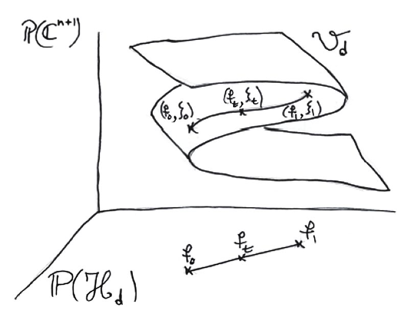
Building on the Shub-Smale homotopy algorithm, there has been exciting progress
here. As with Shub-Smale, the newer path-following algorithms approximate a path,
starting from a given pair (g, ξ) where ξ = (ξ0 , ..., ξn ) and g(ξ) = 0, and output (f, ξ ∗ )
where ξ ∗ is an approximate zero of f . 17
The idea is to lift the “line” segment
ft = (1 − t)g + tf, t ∈ [0, 1]
to the variety Vd = {(f, ξ)|f (ξ) = 0}. Note that f0 = g , and that f1 = f , the system
to be solved.
Sketch by Jean-Pierre Dedieu
17
The polynomial systems considered are homogeneous (for good scaling properties) and the ambient
spaces, projective (for compactness). Here g and f are systems of n homogeneous polynomials in n + 1
variables of degree d = (d1 , ..., dn ).
18By the implicit function theorem, this lift exits if the line does not intersect the dis-
criminant variety of polynomial systems that have zeros with multiplicities. These
algorithms approximate the lifting.
To steer clear of the singular variety of ill-posed pairs (i.e., pairs (f, ξ) where ξ is a
multiple zero of f ), they take into account the condition along the way. The condition
will determine appropriate step size at each stage and hence running time.
Major considerations are: how to choose good initial pairs, how to construct good
partitions (for approximating the path and steering clear of the singular variety), how
to define measures of condition.
In two additional papers Bezout VI [Shu09] and Bezout VII [BS09], Shub and Car-
los Beltrán present an Adaptive Linear Homotopy (ALH) algorithm with incremental
time step dependent on the inverse of a normalized condition number squared.
Beltrán and Luis Miguel Pardo [BP11] show how to compute a random starting pair
yielding a uniform Las Vegas algorithm, polynomial time on average. Utilizing the
numerical algebraic geometry package Macaulay2, the randomized algorithm was im-
plemented by Beltrán and Anton Leykin [BL12].
Bürgisser and Cucker give a hybrid deterministic algorithm which is almost polynomial
time on average [BC11]. Let D be the maximum of the degrees, di. Then for D ≤ n
the algorithm is essentially the ALH of Beltrán and Shub with initial pair:
√
g = (g1 , ..., gn ) where gi (x0 , ..., xn ) = 1/ 2n(x0 di − xi di ) and ζ = (1, ..., 1).
And for D > n, the algorithm calls on Renegar’s symbolic algorithm [Ren89].
The algorithm takes N (loglogN ) arithmetic steps on average, coming close to answering
Smale’s question in the affirmative.
For a tutorial on the subject of this section, see [BS12].
1910 Postscript: Who Invented the Condition Num-
ber?
It is clear that Alan Turing was first to explicitly formalize a measure that would cap-
ture the informal notion of condition (of solving a linear system) and to call this mea-
sure a condition number. Formalizing what’s “in the air” serves to illuminate essence
and chart new direction. However, ideas in the air have many proprietors.
To find out more about the origins of the spectral condition number, I emailed a number
of numerical analysts.
I also looked at many original papers. The responses I received, and related readings,
uncover a debate concerning the origins of the (concept of) condition number not
unlike the debate surrounding the origins of the general purpose computer —with
Turing and von Neumann figuring central to both. (For an insightful assessment of the
latter debate see Mike Shub’s article, “Mysteries of Mathematics and Computation”
[Shu94].)
Gauss himself [Gau03] is referenced for considering perturbations and precondition-
ing. Pete Stewart points to Helmut Wittmeyer [Wit36] in 1936 for some of the earliest
perturbation bounds where products of norms appear explicitly. In 1949, John Todd
[Tod50] explicitly focused on the notion of condition number, citing Turing’s N and
M condition numbers and the implicit von Neumann-Goldstine measure, which he
called the P-condition number (P for Princeton).
Beresford Parlett tells me that “the notion was ‘in the air’ from the time of Turing and
von Neumann et. al.,” that the concept was used by George Forsythe in a course he
took from him at Stanford early in 1959 and that Wilkinson most surely “used the con-
cept routinely in his lectures in Ann Arbor [summer, 1958].” The earliest explicit def-
inition of the spectral condition number I could find in writing was in Alston House-
holder’s 1958 SIAM article [Hou58] (where he cites Turing) and then in Wilkinson’s
book [Wil63], p.91).
By far, the most informative and researched history can be found in Joe Grcar’s 76
page article, “John von Neumann’s Analysis of Gaussian Elimination and the Origins
of Modern Numerical Analysis” [Grc11]. Here he uncovers a letter from von Neumann
to Goldstine (dated January 11, 1947) that explicitly names the ratio of the extreme
singular values as ℓ. Why this was not included in their paper [vNG47] or made explicit
20in their error bounds is a mystery to me.18 Grcar chalks this up to von Neumann using
his speeches (e.g. [vN89]) to expound on his ideas, particularly those given to drum
up support for his computer project at the Institute for Advanced Study.19
Grcar’s article definitely puts von Neumann at center stage. Of von Neumann’s role as
a key player in this area there is no doubt. However, Grcar also implies, that Turing’s
work on rounding error, and the condition number, was prompted by Turing’s meeting
with von Neumann in Princeton in January 1947. Indeed, prominently on page 630 he
says, “No less than Alan Turing produced the first derivative work from the inversion
paper.”
This flies in the face of all we know about Alan Turing’s singular individuality, both in
personality and in research. In their personal remembrances of Turing, both Wilkinson
[Wil71], who worked closely with him at the NPL in Teddington, and Max Newman
[New55], earlier at Cambridge and Bletchley and later in Manchester, point to Turing’s
“strong predilection for working everything out from first principles, usually in the
first instance without consulting any previous work on the subject, and no doubt it
was this habit which gave his work that characteristically original flavor.”
It also flies in the face of fact. As recounted by Wilkinson, Turing’s experience with
his team at the NPL, prior to meeting von Neumann in Princeton in 1947, was the
stimulus for his paper:
… some time after my arrival [at the NPL in 1946], a system of 18 equa-
tions arrived in Mathematics Division and after talking around it for some
time we finally decided to abandon theorizing and to solve it. … The op-
eration was manned by [Leslie] Fox, [Charles] Goodwin, Turing, and me,
and we decided on Gaussian elimination with complete pivoting. Turing
was not particularly enthusiastic, partly because he was not an experienced
performer on a desk machine and partly because he was convinced that it
18
Joe was also kind enough to illuminate for me in detail how one could unravel von Neumann’s and
Goldstine’s error analysis for the general case in their paper.
Many authors have cited the obtuseness and non-explicitness. For example, Edelman, in his PhD
thesis [Ede89], recasts von Neumann’s and Goldstine’s ideas in modern notation given “the difficulty of
extracting the various ideas from their work’’ and cites Wilkinson’s referring to the paper’s “indigestibil-
ity.”
19
An unpublished and undated paper by Goldstine and von Neumann [GvN63] containing material
presented by von Neumann in various lectures going back to 1946, but clearly containing later perspec-
tives as well, explicitly singles out (on page 14) ℓ as the “figure of merit.” Also interesting to me, in the
same paragraph, are the words “loss of precision” connected to the condition number, possibly for the
first time.
21would be a failure. … the system was mildly ill-conditioned, the last equa-
tion had a coefficient of order 10−4 … and the residuals were … of order
10−10 , that is of the size corresponding to the exact solution rounded to
ten decimals. …
... I’m sure that this experience made quite an impression on him and
set him thinking afresh on the problem of rounding errors in elimination
processes. About a year later he produced his famous paper “Rounding-off
errors in matrix process” ...20
Velvel Kahan (also a Turing Award recipient), in his 1966 paper [Kah66] and in a
lengthy phone conversation (August 2011), asserts that von Neumann and Goldstine
were misguided in their approach to matrix inversion (by computing A−1 from the
formula A−1 = (AT A)−1 AT ).
Kahan’s assessment of Turing is a fitting conclusion to this paper:
A more nearly modern error-analysis was provided by Turing (1948) in a pa-
per whose last few paragraphs foreshadowed much of what was to come,
but his paper lay unnoticed for several years until Wilkinson began to pub-
lish the papers which have since become a model of modern error-analysis.21
11 Acknowledgements
Much of what I know about Alan Turing’s life comes from Andrew Hodges’ definitive
biography, Alan Turing: the Enigma [Hod92]. I had the pleasure to discuss the material
in this paper with Hodges at the Turing Centenary Conference, CiE 2012 - How the
World Computes, at the University of Cambridge, England. I thank the organizers of
the conference, and in particular, Barry Cooper, for inviting me to speak.
Mike Shub and Steve Smale are the architects, sans pareil, of the most fundamental
results in the area of complexity and real computation. My perspectives are clearly
20
On June 23, 2012, at the Turing Centenary Conference in Cambridge, England, Andrew Hodges told
me that in Turing’s 1945 paper on the design of the ACE programmable computer (classified for many
years) there is a discussion of the need for accurate numerical computations, and Gaussian Elimination
is one of the examples given.
21
Kahan is referring to backward error analysis which, rather than estimating the errors in a computed
solution of a given problem instance (i.e., forward error analysis), estimates the closeness of a nearby
problem instance whose exact solution is the same as the approximate computed solution of the original.
Grcar [Grc11] also points to the von Neumann and Goldstine paper as a precursor to this notion as well.
22fashioned by my long time collaboration with them. Jim Renegar, who constantly
amazes with his deep insights and beautiful algorithms, has been a constant sounding
board for me.
I would like to thank the Mathematics Department of the University of Toronto for
inviting me to be Dean’s Distinguished Visitor during the Fields Institute Program
on the Foundations of Computational Mathematics, Fall 2009. There I co-taught a
course with my collaborator Felipe Cucker, and learned about new advances concern-
ing condition from lectures given by Felipe and Peter Bürgisser whose influence is
apparent here. Their forthcoming book, Condition [BC12], is certain to become the
bible in this area. For an excellent survey paper see [Bür10].
Jean-Pierre Dedieu, who celebrated his 60th birthday during the Fields program, in-
spired us all with his beautiful lectures on Complexity of Bezout’s Theorem and the
Condition Number. We lost Jean-Pierre during the Centenary Year of Alan Turing. I
dedicate this paper to him.
References
[BC11] Peter Bürgisser and Felipe Cucker. On a problem posed by Steve Smale.
Annals of Mathematics, 174(3):1785–1836, 2011.
[BC12] Peter Bürgisser and Felipe Cucker. Complexity. to appear, 2012.
[BCL08] Peter Bürgisser, Felipe Cucker, and Martin Lotz. The probability that a
slightly perturbed numerical analysis problem is difficult. Math. Comput.,
77(263):1559–1583, 2008.
[BCSS96] Lenore Blum, Felipe Cucker, Michael Shub, and Stephen Smale. Algebraic
settings for the problem “P ̸= N P ?”. In The Mathematics of Numerical
Analysis, volume 32 of Lectures in Applied Mathematics, pages 125–144. Amer.
Math. Soc., 1996.
[BCSS98] Lenore Blum, Felipe Cucker, Michael Shub, and Stephen Smale. Complex-
ity and Real Computation. Springer, New York, 1998.
[BL12] Carlos Beltrán and Anton Leykin. Certified numerical homotopy tracking.
Experiment. Math., 21(1):69–83, 2012.
23[Blu90] Lenore Blum. Lectures on a theory of computation and complexity over
the reals (or an arbitrary ring). In E. Jen, editor, 1989 Lectures in the Sciences
of Complexity II, pages 1–47. Addison Wesley, 1990.
[Blu91] Lenore Blum. A theory of computation and complexity over the real num-
bers. In I. Satake, editor, Proceedings of the International Congress of Math-
ematicians (ICM 1990), volume 2, pages 1942–1507. Springer-Verlag, 1991.
[Blu04] Lenore Blum. Computing over the reals: Where Turing meets New-
ton. Notices of the American Mathematical Society, 51:1024–1034, 2004.
http://www.ams.org/notices/200409/fea-blum.pdf.
[Blu12] Lenore Blum. Alan Turing and the other theory of computation. In S.Barry
Cooper and Jan van Leeuwen, editors, The Selected Works of A.M. Turing:
His Work and Impact. Elsevier, 2012.
[BMvN63] Valentine Bargmann, Deane Montgomery, and John von Neumann. Solu-
tion[s] of linear systems of high order. In A. H. Taub, editor, John von
Neumann Collected Works, volume 5, pages 421–478. Macmillan, New York,
1963. Report prepared for Navy Bureau of Ordnance, 1946.
[BP11] Carlos Beltrán and Luis Miguel Pardo. Fast linear homotopy to find
approximate zeros of polynomial systems. Found. Comput. Math.,
11(1):95–129, February 2011.
[BS86] Lenore Blum and Michael Shub. Evaluating rational functions: Infi-
nite precision is finite cost and tractable on average. SIAM J. Comput.,
15(2):384–398, May 1986.
[BS09] Carlos Beltrán and Michael Shub. Complexity of Bezout’s theorem
VII: Distance estimates in the condition metric. Found. Comput. Math.,
9(2):179–195, March 2009.
[BS12] Carlos Beltrán and Michael Shub. The complexity and geometry of nu-
merically solving polynomial systems. preprint, 2012.
[BSS89] Lenore Blum, Michael Shub, and Stephen Smale. On a theory of compu-
tation and complexity over the real numbers: NP-completeness, recursive
functions and universal machines. Bulletin of the American Mathematical
Society, 21:1–46, 1989.
24[Bür10] Peter Bürgisser. Smoothed analysis of condition numbers. In Proceedings of
the International Congress of Mathematicians (ICM 2010), volume 4, chapter
166, pages 2609–2633. World Scientific, 2010.
[CSS94] Felipe Cucker, Michael Shub, and Stephen Smale. Separation of com-
plexity classes in Koiran’s weak model. Theoretical Computer Science,
133(1):3–14, 1994.
[Cuc02] Felipe Cucker. Real computations with fake numbers. J. Complexity,
18(1):104–134, 2002.
[Dan47] George B. Dantzig. Origins of the simplex method. In S.G. Nash, editor, A
History of Scientific Computing, pages 141–151. ACM Press, New York, 1990
(1947).
[Dem87] James Weldon Demmel. On condition numbers and the distance to
the nearest ill-posed problem. Numerische Mathematik, 51:251–289, 1987.
10.1007/BF01400115.
[DSTT02] John Dunagan, Daniel A. Spielman, Teng, and Shang-Hua Teng. Smoothed
analysis of Renegar’s condition number for linear programming. In In
SIAM Conference on Optimization, 2002.
[Ede88] Alan Edelman. Eigenvalues and condition numbers of random matrices.
SIAM J. Matrix Anal. Appl., 9(4):543–560, December 1988.
[Ede89] Alan Edelman. Eigenvalues and Condition Numbers of Random Matrices.
PhD thesis, MIT, 1989. http://math.mit.edu/~edelman/thesis/thesis.pdf.
[EY36] Carl Eckart and Gale Young. The approximation of one matrix by another
of lower rank. Psychometrika, 1(3):211–218, September 1936.
[Fed69] Herbert Federer. Geometric measure theory. Grundlehren der mathema-
tischen Wissenschaften. Springer, 1969.
[FHW48] Leslie Fox, Harry D. Huskey, and James Hardy Wilkinson. Notes on the
solution of algebraic linear simultaneous equations. Quarterly Journal of
Mechanics and Applied Mathematics, 1:149–173, 1948.
[Gau03] Carl Friedrich Gauss. Letter to Gerling, December 26, 1823. Werke,
9:278–281, 1903. English translation, by George E. Forsythe, Mathematical
Tables and Other Aids to Computation, volume 5 (1951) pp. 255-258.
25[Grc11] Joseph F. Grcar. John von Neumann’s analysis of Gaussian elimination and
the origins of modern numerical analysis. SIAM Rev., 53:607–682, 2011.
[GvN63] Herman H. Goldstine and John von Neumann. On the principles of large
scale computing machines (unpublished). In Abraham H. Taub, editor,
John von Neumann Collected Works, volume 5, pages 1–33. Macmillan, New
York, 1963.
[Hig02] Nicholas J. Higham. Accuracy and Stability of Numerical Algorithms. Society
for Industrial and Applied Mathematics, Philadelphia, PA, USA, second
edition, 2002.
[Hod92] Andrew Hodges. Alan Turing: the Enigma. Vintage, 1992.
[Hot43] Harold Hotelling. Some new methods in matrix calculation. Ann. Math.
Statist., 14(1):1–34, 1943.
[Hou58] Alston S. Householder. A class of methods for inverting matrices. Journal
of the Society for Industrial and Applied Mathematics, 6:189–195, June, 1958.
[Kah66] William M. Kahan. Numerical linear algebra. Canadian Mathematical
Bulletin, 9:757–801, 1966.
[KM72] Victor Klee and George J. Minty. How good is the simplex algorithm? In
O. Shisha, editor, Proceedings of the Third Symposium on Inequalities, volume
III of Inequalities, pages pp. 159–175, New York, 1972. Academic Press.
[Kos88] Eric Kostlan. Complexity theory of numerical linear algebra. J. Comput.
Appl. Math., 22(2-3):219–230, June 1988.
[New55] Maxwell H. A. Newman. Alan Mathison Turing. 1912-1954. Biographical
Memoirs of Fellows of the Royal Society, 1:253–263, 1955.
[PER89] Marian. B. Pour-El and J. Ian Richards. Computability in analysis and physics.
Perspectives in mathematical logic. Springer Verlag, 1989.
[Ren88a] James Renegar. A faster PSPACE algorithm for deciding the existential
theory of the reals. In Proceedings of the 29th Annual Symposium on Foun-
dations of Computer Science, pages 291–295. IEEE Computer Society, 1988.
[Ren88b] James Renegar. A polynomial-time algorithm, based on Newton’s method,
for linear programming. Mathematical Programming, 40:59–93, 1988.
26[Ren89] James Renegar. On the worst-case arithmetic complexity of approximat-
ing zeros of systems of polynomials. SIAM J. Comput., 18(2):350–370,
April 1989.
[Ren95a] James Renegar. Incorporating condition measures into the complexity
theory of linear programming. SIAM Journal on Optimization, 5:5–3, 1995.
[Ren95b] James Renegar. Linear programming, complexity theory and elementary
functional analysis. Mathematical Programming, 70:279–351, 1995.
[San04] Luis Antonio Santaló. Integral Geometry and Geometric Probability.
Cambridge Mathematical Library. Cambridge University Press, 2004.
[Shu94] Michael Shub. Mysteries of mathematics and computation. The Mathe-
matical Intelligencer, 16:10–15, 1994.
[Shu09] Michael Shub. Complexity of Bezout’s theorem VI: Geodesics in the con-
dition (number) metric. Found. Comput. Math., 9(2):171–178, March 2009.
[Sma81] Stephen Smale. The fundamental theorem of algebra and complexity the-
ory. Bull. Amer. Math. Soc., 4(1):1–36, 1981.
[Sma97] Stephen Smale. Complexity theory and numerical analysis. Acta Numerica,
6:523–551, 1997.
[Sma00] Stephen Smale. Mathematical problems for the next century. In V. I.
Arnold, M. Atiyah, P. Lax, and B. Mazur, editors, Mathematics: Frontiers
and Perspectives, pages 271–294. American Mathematical Society, 2000.
[SS94] Michael Shub and Stephen Smale. Complexity of Bezout’s theorem V:
Polynomial time. Theoretical Computer Science, 133:141–164, 1994.
[ST01] Daniel A. Spielman and Shang-Hua Teng. Smoothed analysis of algorithms:
why the simplex algorithm usually takes polynomial time. In Journal of the
ACM, pages 296–305, 2001.
[Tar51] Alfred Tarski. A Decision Method for Elementary Algebra and Geometry.
University of California Press, 1951.
[TB97] Lloyd N. Trefethen and David Bau. Numerical linear algebra. SIAM, 1997.
[Tod50] John Todd. The condition of a certain matrix. Proceedings of the Cambridge
Philosophical Society, 46:116–118, 1950.
27[Tod68] John Todd. On condition numbers. In Programmation en Mathématiques
Numériques, Besançon, 1966, volume 7 (no. 165) of Éditions Centre Nat.
Recherche Sci., Paris, pages 141–159, 1968.
[Tur36] Alan Mathison Turing. On computable numbers, with an application to
the Entscheidungsproblem. Proceedings of the London Mathematical Society,
2, 42(1):230–265, 1936.
[Tur45] Alan Mathison Turing. Proposal for development in the Mathematics Di-
vision of an Automatic Computing Engine (ACE). Report E.882, Executive
Committee, inst-NPL, 1945.
[Tur48] Alan Mathison Turing. Rounding-off errors in matrix processes. Quarterly
Journal of Mechanics and Applied Mathematics, 1:287–308, 1948.
[vN89] John von Neumann. The principles of large-scale computing machines.
Annals of the History of Computing, 10(4):243–256, 1989. Transcript of lecture
delivered on May 15, 1946.
[vNG47] John von Neumann and Herman H. Goldstine. Numerical inverting of
matrices of high order. Bulletin of the American Mathematical Society,
53(11):1021–1099, November 1947.
[Wei00] Klaus Weihrauch. Computable Analysis: An Introduction. Texts in Theo-
retical Computer Science. Springer, 2000.
[Wey39] Hermann Weyl. On the volume of tubes. Am. J. Math., 61:461–472, 1939.
[Wil63] James Hardy Wilkinson. Rounding Errors in Algebraic Processes. Notes on
Applied Science No. 32, Her Majesty’s Stationery Office, London, 1963.
Also published by Prentice-Hall, Englewood Cliffs, NJ, USA. Reprinted
by Dover, New York, 1994.
[Wil71] James Hardy Wilkinson. Some comments from a numerical analyst. Jour-
nal of the ACM, 18(2):137–147, 1971. 1970 Turing Lecture.
[Wit36] Helmut Wittmeyer. Einfluß der Änderung einer Matrix auf die Lösung des
zugehörigen Gleichungssystems, sowie auf die charakteristischen Zahlen
und die Eigenvektoren. Z. Angew. Math. Mech., 16:287–300, 1936.
28You can also read