Assessment of king scallop stock status for selected waters around the English coast 2019/2020 - Annexe - Andrew Lawler and Nikolai Nawri February ...

Assessment of king scallop stock status
for selected waters around the English
coast 2019/2020 – Annexe

Andrew Lawler and Nikolai Nawri

February 2021

© Crown copyright 2020
This information is licensed under the Open Government Licence v3.0. To view this licence,
visit www.nationalarchives.gov.uk/doc/open-government-licence/

This publication is available at www.gov.uk/government/publications

www.cefas.co.uk

Cefas Document Control

Submitted to: Helen Hunter

Date submitted: 14th April 2021

Project Manager: Nicki Hawkes

Report compiled by: Andy Lawler and Nikolai Nawri

Quality control by: Stuart Reeves

Approved by and date: 25th March 2021

Version: V2.0

 Lawler, A. & Nawri, N., (2021). Assessment of king scallop stock
Recommended citation
 status for selected waters around the English coast 2019/2020 –
for this report:
 Annexe. Cefas Project Report for Defra,+ 32 pp.

 Version control history

Version Author Date Comment

V1.0 Lawler, A. & Nawri, N 25/01/21 1st draft
V2.0 Lawler, A. & Nawri, N 25/03/21 2nd draft

Contents

1. Scallop biological sampling procedure.......................................................................... 3

 1.1. Methodology .......................................................................................................... 3

 1.2. Sampling targets.................................................................................................... 4

 1.3. Data raising process .............................................................................................. 4

2. Dredge survey design ................................................................................................... 5

 2.1. Terminology ........................................................................................................... 5

 2.2. Identification of scallop beds ................................................................................. 7

 2.3. Station selection .................................................................................................... 8

3. Dredge survey data processing .................................................................................. 12

 3.1. Scallop density raising ......................................................................................... 12

 3.2. Sample processing .............................................................................................. 12

 3.3. Swept area estimation ......................................................................................... 13

 3.4. Substrate-specific dredge efficiency .................................................................... 14

4. Underwater television survey ...................................................................................... 16

 4.1. Methodology ........................................................................................................ 16

 4.1.1. Survey design............................................................................................... 16

 4.1.2. Video processing .......................................................................................... 18

 4.2. Results ................................................................................................................ 18

5. Supporting research and development ....................................................................... 20

 5.1. Dredge efficiency estimates................................................................................. 20

 5.2. Biomass estimates from UWTV ........................................................................... 22

 5.2.1. Camera system ............................................................................................ 22

 5.2.2. Camera efficiency ......................................................................................... 22

 5.2.3. Population structure ..................................................................................... 23

 1

5.2.4. Connectivity between dredged and un-dredged areas ................................. 23

6. Dredge survey of Bed 7.d.2 in Area 27.7.d.S ............................................................. 23

 6.1. Dredge survey 2018 ............................................................................................ 23

 6.2. Raised biomass estimates and uncertainty ......................................................... 24

 6.3. Size composition from dredge survey.................................................................. 26

 6.4. Conclusion ........................................................................................................... 26

7. References ................................................................................................................. 27

Tables

Table 2.1: Minimum number of cells used to determine whether a block is deemed valid for
being surveyed. ................................................................................................................... 8

Table 3.1: Number of tows by ground type in each bed with proportion described by the
survey vessel skipper as having significant amounts of flint or cobbles. ............................ 15

Table 4.1: Summary of the 2017 and 2019 UWTV survey results. Densities are given as
numbers per 100 m2. ......................................................................................................... 19

Table 4.2: Abundance of scallops in un-dredged zones surveyed by UWTV, together with
harvestable biomass and spawning stock biomass. .......................................................... 20

Table 6.1: Sampling summary from the 2018 dredge survey in Bed 7.d.2......................... 24

Table 6.2: Biomass estimate for Bed 7.d.2 based on the 2018 dredge survey. ................. 26

Figures

Figure 2.1: An example scallop dredge bed (red outline) with 0.1-degree blocks (black)
and 0.025-degree cells (blue). ............................................................................................. 6

Figure 2.2: Valid (blue) and invalid (red) blocks in Beds 7.e.1-8 ( ICES Division 27.7.e),
and Bed 7.f.1 (Division 27.7.f), along with the number of cells within each block. ............... 9

Figure 2.3: Valid (blue) and invalid (red) blocks in Bed 7.d.1 (Area 27.7.d.N), along with the
number of cells within each block. ..................................................................................... 10

 2

Figure 2.4: Valid (blue) and invalid (red) blocks in Bed 4.b.1-2 (Area 27.4.b.S), along with
the number of cells within each block. ............................................................................... 11

Figure 4.1: The UWTV survey un-dredged zones as defined in 2017 (black outlines) and
2019 (red outlines). ............................................................................................................ 17

Figure 4.2: Estimated density (numbers m-2) from the 2017 and 2019 UWTV surveys by
block in un-dredged zones of the assessment areas. ........................................................ 19

Figure 6.1: Sampled blocks in Bed 7.d.2 (Area 27.7.d.S) in 2018. Block shading indicates
the total number of stations within each block 0 =grey, 1=blue.......................................... 24

Figure 6.2: Biomass of harvestable (round shell length ≥ 110 mm, the MLS) scallops in
Bed 7.d.2 (Area 27.7.d.S) in 2018. .................................................................................... 25

Figure 6.3: Numbers (millions) per 5-mm length class for the scallop population in Bed
7.d.2 in 2018. The vertical line represents MLS. ................................................................ 26

1. Scallop biological sampling procedure

1.1. Methodology
The fishing industry proposed a methodology for the sampling procedure, which is a
modification of an earlier scheme:

 1. Cefas identifies sampling opportunities based on regular reports of the positions of
 participating vessels from the Vessel Monitoring Scheme (VMS) and requests a
 length or age sample from the processor.
 2. The processor contacts the vessel operator by phone or internet-based messaging
 and requests a sample to be collected from the next haul.
 3. The vessel crew collect a bag of scallops in a labelled and coloured bag (to aid
 identification at the processor) and land it along with the rest of the catch. Length
 samples are retained in red bags, and those for age determination are retained in a
 blue bag.
 4. At the processors, the industry staff measure the length samples (height of round
 shell perpendicular to hinge) and return the size distributions along with sample
 weight and sample details to Cefas. Age samples are processed at the factory as
 per the usual procedure, but flat shells are sent to Cefas for age determination.
 5. A supplementary and opportunistic method was introduced, where samples are pre-
 ordered by the processor contacts in consideration of target shortfalls.

 3

In the laboratory low power microscopes are used to confirm age, as growth rings
observed with the naked eye have shown to be unreliable in the English Channel. Initial
ages are checked and, where discrepancies exist between readers, are determined by
consensus.

1.2. Sampling targets
The spatial distribution of fishing effort and catches within each fishing season can be
difficult to predict and appears to be influenced by irregular recruitment events. VMS data
were used to define ICES statistical rectangles where fishing activity had occurred over the
past 8 years and warranted sampling. Sampling targets in the first year (2017) were set at
5 length samples per rectangle per quarter year, where one of the length samples is
retained for subsequent age determination to facilitate the construction of an age-length
key for each rectangle. From 2018, sampling targets were revised to better reflect fishing
patterns as defined by reported landings. One sample was requested for a threshold of 1
tonne of scallop landed per rectangle and then another for each subsequent 50 tonnes. To
provide an improved estimation of age structure. two age samples were requested for
every 3 length samples.

In a process parallel to that used by finfish stock assessments, estimates of the age
composition of landings were obtained from length distributions through conversion to
ages by means of an age-length key.

Given the limited mobility of scallops, together with pre-existing knowledge on the
patchiness of scallop settlement and variability in growth rates, the sampling strata
employed for scallops are much smaller than those for finfish.

The basic strata for the targeting of age and length are ICES statistical rectangles and
reported landings. Samples are requested from a vessel when it is observed to be fishing
in an area on a given day (using VMS data). The unit of sampling is therefore a
combination of vessel, rectangle and day.

1.3. Data raising process

Age-length key (ALK)

 1. From the age samples (blue-bag), 5 shells per 5-mm length class are retained for
 age-determination.

 4

2. Within each 5-mm length class, the proportion of each age was determined to give
 an ALK for each rectangle-quarter stratum.
 3. To fill any strata for which there were missing ALKs, all age (blue-bag) samples
 were pooled to the quarter - assessment area level to generate an ALK for each un-
 sampled rectangle within that assessment area.
Length distribution

 4. Sample length distributions (LDs) were raised to the reported catch of the vessel
 within the day, using the ratio of reported sample weight to landings.
 5. Sample LDs and weights from step 4 were aggregated to the level of rectangle and
 quarter.
 6. The pooled LDs from step 5 were raised to the total UK landings for that rectangle
 and quarter using the ratio of the sampled weight to total landings.
 7. Not all strata with landings records had length samples. Missing strata were
 assumed to come from the same length distribution as the aggregate quarter –
 assessment area. The LDs from step 6 were pooled and then raised to each
 missing stratum using the ratio of sampled weight to strata landings.
 8. Numbers in each size class from step 7 were summed within each stock
 assessment area and sampling season (quarter 4 of the previous calendar year
 plus quarters 1-3 of the current year) to give total numbers in each size class per
 assessment area and sampling season.
Age distribution

 9. For directly sampled strata, the raised rectangle-quarter numbers-at-length were
 multiplied by the corresponding ALK and then summed to give the total numbers-at-
 age per rectangle-quarter
 10. For un-sampled strata, the in-fill LDs (step 7) were multiplied by the in-fill ALK (step
 3) and summed to give numbers-at-age per un-sampled rectangle-quarter.
 11. These numbers-at-age were summed over all quarters and rectangles within each
 stock assessment area and for each sampling season to give total removals-at-age
 per assessment area and sampling season.

2. Dredge survey design

2.1. Terminology
The following spatial areas were used during the survey design process:

 • Bed – A polygon representing a fished scallop ground, identified using Vessel
 Monitoring System (VMS) data.

 5

• Block – A regular coordinate grid of 0.1-by-0.1-degree rectangles, with an
 approximate area of 80 km2.
 • Cell – A regular coordinate grid of 0.025-by-0.025-degree rectangles, with an
 approximate area of 5 km2 and a maximum of 16 cells per block (4 by 4). This is the
 scale to which VMS data are aggregated as part of the survey design methodology.
 Mid-points of cells are used as potential sampling positions, randomly selected as
 part of the dredge survey design. This also forms the grid over which the data are
 raised to calculate the bed biomass and age-length population structure.
 • Valid cell – A cell for which fishing activity has been identified based on VMS data.
 • Valid block – A block with a specific minimum number of valid cells.

These concepts are graphically presented in Figure 2.1.

Figure 2.1: An example scallop dredge bed (red outline) with 0.1-degree blocks (black) and
0.025-degree cells (blue).

 6

2.2. Identification of scallop beds
VMS data for fishing trips during the 2009-2016 period, during which scallop dredges were
deployed, were used to identify the location of scallop grounds targeted by the commercial
scallop dredge fleet in the English Channel. For the first four years of data, only vessels
with lengths of at least 15 m were available, but changes to the VMS scheme enabled all
vessels with lengths of 12 m and above to be included from 2013.

VMS data were processed as follows:

 • Vessels were assumed to be fishing when the reported speed was between 1 and 5
 knots. This speed range was used to remove records where vessels were likely to
 be transiting between grounds, or in harbour.
 • VMS data were aggregated to cell level (on a 0.025-degree grid). Cells with less
 than 10 reported positions over the full-time series were removed.
 • A measure of landings per unit effort (LPUE) was derived for each VMS position by
 dividing the reported trip landings for the relevant combination of vessel-day-
 rectangle by the fishing hours estimated from VMS data for the same strata.

Bed boundary polygons were created using the R function ashape from the alphahull
package. This function uses the algorithm defined by (Edelsbrunner, et al., 1983) to
construct an α-shape around a set of points, in this case VMS points (cells), based upon
the Delaunay triangulation.

The resulting α-shape was converted to a polygon (bed outline) representing a scallop
fishing ground. Within each bed there are patches where VMS data are absent. These are
represented as areas without valid cells (Figure 2.1). When aggregating the survey results
within each scallop bed, only those cells with scallop-related VMS points are used. The
assumption is that no commercial fishing (at least by vessels that are part of the VMS
scheme) takes place in these cells, and that therefore there are no scallops in those cells
that are accessible to standard fishing gear.

For the 2017 survey season, eight scallop beds within ICES Division 27.7.e, and one
scallop bed within Division 27.7.d were defined using the above approach. In 2018 three
additional scallop beds were identified using the same time series of VMS data, one in
Division 27.7.f and two in Division 27.4.b. Following recent expansion of the fishery in
Division 27.7.d., a further bed (7.d.2.) was identified by including 2017 fishing activity in the
VMS time series.

 7

2.3. Station selection
A random stratified sampling design was used. As it is not clear if scallop density is
randomly distributed across the whole bed, it was considered important to ensure broad
spatial coverage of the sampling design. Therefore, within each bed, blocks were used to
represent the different strata. Broad spatial coverage is provided by ensuring that most
blocks are sampled. Within each block, one valid cell was selected at random, the
midpoint of which was a potential sampling position. This procedure ensured stations were
only placed in areas commercially fished for scallops, and generated mean tow position
separations in line with those suggested by earlier scoping work carried out in 2016
(Lawler, 2017; unpublished).

For the available survey time, it was not possible to sample each block which intersected
the bed boundary. Many blocks, particularly around the boundary had very few valid cells
contained within them (Figure 2.2, Figure 2.3, and Figure 2.4). A protocol was therefore
developed to ensure that the sampled blocks represented as many of the valid cells as
possible within the sampling time frame. For each bed, a threshold number of valid cells
per block was established such that more than 85% of the cells within each bed fell inside
the sampled blocks. Table 2.1 gives the minimum number of valid cells per bed. This
ensures that the main fishing areas are sampled within each bed, and the number of
stations are consistent with the optimal tow separation suggested by the earlier scoping
work. However, it does also mean that densities around the boundary of each bed are less
well sampled, which could introduce bias into the approach, if there is a steeper gradient of
density along bed boundaries than in the main fishing grounds.

Table 2.1: Minimum number of cells used to determine whether a block is deemed valid for
being surveyed.

 Bed Total Cell Blocks Cells % Cells Number
 Number of Threshold Dropped Dropped Dropped of
 Intersecting Stations
 Blocks

 4.b.1 38 4 15 33 11 23
 4.b.2 8 2 4 6 20 4
 7.d.1 100 8 31 91 8 69
 7.e.1 32 5 11 36 14 21
 7.e.2 47 9 13 60 11 34
 7.e.3 3 2 1 2 13 2
 7.e.4 46 6 15 65 14 31
 7.e.5 30 4 11 27 11 19

 8

Bed Total Cell Blocks Cells % Cells Number
 Number of Threshold Dropped Dropped Dropped of
 Intersecting Stations
 Blocks

 7.e.6 5 2 2 3 11 3
 7.e.7 11 3 4 9 11 7
 7.e.8 37 6 15 47 13 22
 7.f.1 21 5 8 19 12 13

Figure 2.2: Valid (blue) and invalid (red) blocks in Beds 7.e.1-8 ( ICES Division 27.7.e), and
Bed 7.f.1 (Division 27.7.f), along with the number of cells within each block.

 9

Figure 2.3: Valid (blue) and invalid (red) blocks in Bed 7.d.1 (Area 27.7.d.N), along with the
number of cells within each block.

 10

Figure 2.4: Valid (blue) and invalid (red) blocks in Bed 4.b.1-2 (Area 27.4.b.S), along with the
number of cells within each block.

For the 2017 survey season, Industry collaborators were keen to contribute to the tow
position selection process in line with some other collaborative surveys. It was agreed that
industry could select 25% of the tow positions per bed. Therefore, 75% of the valid blocks
were selected at random, from which a suite of scientifically derived station tow positions
was selected by randomly choosing valid cells from the selected block. No rationale
behind the choice of industry location was sought or provided, but the basic assumption
was that these were not selected at random, but rather on prior knowledge. The inclusion
of subjectively chosen station points has the potential to bias the result. If positions of
known high density are selected, then high-density locations will be over-represented and
are likely to bias the total population estimate upwards. Conversely over-representation of
low-density areas will lead to an under-estimate of the population. Such bias is likely to be
realised most strongly if all stations are pooled together to generate an average density
per bed. Indeed, this approach would violate the statistical integrity of any abundance

 11

estimate. From 2018 onwards, tow selection was entirely by random selection, although
the focus is still on the main fishing areas.

3. Dredge survey data processing

3.1. Scallop density raising
The stratified random design dictated that the data were processed by block as the
sampling strata. The density estimate from stations within a block were considered
representative of the surface area of the block, and the block mean density was used if
more than one station was in a single block. The valid surface area of each block is the
sum of the surface area of all valid cells. Total block abundance (in numbers) is then given
by

 = ∑ ,

where c are the valid cells, is the areal number density, and is the surface area of
each cell.

There were however un-sampled blocks which had a surface area defined by the valid
cells within that block. The stock lying within the un-sampled blocks was estimated by
applying the bed-averaged density from the survey stations to the total valid surface area
of the un-sampled blocks.

For the 2017 survey, the remaining issue was how to incorporate the industry-selected
stations within this approach. As we could not guarantee that the industry station locations
had been chosen at random, statistically speaking they could not be used to represent the
mean density for the whole block. Because they were chosen specifically for a site, the
Industry-selected stations could only be used as observations for that specific site (cell).
The science-derived estimate of scallop abundance was used for all cells except for those
were an industry selected station occurred, where the abundance was replaced by that
observed at the industry selected station.

3.2. Sample processing
Sampling was carried out from the dredges on only one side of the vessel, which provided
adequate sampling levels throughout the surveys. As such, samples were raised only to
the catches and area swept by sampled dredges, avoiding the need to consider any
potential bias between starboard and port gears.

 12

The following raising procedure was carried out on the survey data for the commercial
dredge gear:

 1. The sampled length distribution (LD) was raised to the total catch per station, using
 the raising factor calculated as caught weight or numbers over sampled weight or
 numbers for the two catch components, discards (below minimum landing size,
 MLS) and retained.
 2. The catch components were aggregated to get total raised numbers at size by
 station.
 3. The catch density (number m-2) for each station was calculated by dividing the
 count by the swept area of the gear.
 4. The station catch densities from step 3 were raised using the appropriate substrate-
 specific gear efficiency factor to estimate scallop density on the seabed.
 5. For randomly allocated stations, and for blocks which had one or more sampled
 cells, the block mean density per length class was calculated.
 6. For randomly allocated stations, the bed mean density per length class was
 calculated.
 7. Block mean densities were applied to all cells within blocks, where there was at
 least one sampled cell.
 8. Bed mean densities were applied to all cells in all un-sampled blocks.
 9. For the 2017 survey, densities in cells where an industry selected station was
 available were substituted with the density generated for that industry station.
 10. Cell densities were raised to the area of each cell.
 11. Number densities from step 10 were summed within each assessment area to
 generate raised numbers-at-size.

Steps 3 to 11 were repeated with the age converted data, using the sample ALKs to
generate the age profile of the population. The harvestable biomass was calculated for
each assessment area by using the length-weight conversion parameters to calculate
weight-at-length for scallops larger than the MLS. For assessment areas in ICES Divisions
27.4.b and 27.7.e, the MLS is 100 mm round shell length, whilst for ICES Divisions 27.7.d
it is 110 mm.

3.3. Swept area estimation
Internally logging data storage tags (Cefas G5) recording depth and time were attached to
the bridles on the dredges to provide depth profiles and an accurate indication of the time
of deployment. GPS receivers (RoyalTech MBT1100) recorded ship positions. These
loggers provided the positions of the tow tracks with depth profiles of the gear and allowed
the calculation of distance run at each tow position. This integrated method is a more
accurate measure of tow distance than calculating straight line distances between start
and end points, and eliminates potential data recording errors. From 2018, a smooth line

 13

(tensor line) was fitted through the positional information to provide a more accurate
interpretation of the distance run. For some tows, GPS data failed to log. For these,
distance run was calculated as the product of mean tow speed (2.7 knots) and intended
tow duration (15 min). The swept area was then calculated as the sum of all individual
dredge widths (75 cm times the number of dredges), multiplied by the tow distance (2.7
knots times 15 min = 1.25 km). As the data were only raised to the dredges on one side of
the vessel, the number of dredges used in this calculation of swept area only includes
sampled dredges.

3.4. Substrate-specific dredge efficiency
The vessel skipper reports ground type at each survey tow location based on acoustic
information in the wheelhouse and the contents of the dredges. The distribution of these
ground types by bed and survey year is presented in Table 3.1. The skipper-reported
ground types were related to two ground types described by historic depletion studies
carried out by Cefas in the English Channel. These substrate-specific gear efficiencies are
listed in the main part of the report, individually for each assessment area. The data were
therefore adjusted for gear efficiency at each station based upon the skipper determined
ground type, prior to the raising procedure. The assumption of this method is that the
ground types encountered at each tow position were representative of the wider area
(block).

 14

Table 3.1: Number of tows by ground type in each bed with proportion described by the
survey vessel skipper as having significant amounts of flint or cobbles.

 Bed Year Ground Type Total Tows with
 Flint
 Cobbles (%)

 Clean, Some Flint or
 Stones Cobbles
 4.b.1 2018 8 15 23 0.65
 2019 19 3 22 0.14
 2020 22 0 22 0.00
 4.b.2 2018 2 2 4 0.50
 2019 1 1 1 0.00
 2020 2 0 2 0.00
 7.d.1 2017 49 14 63 0.22
 2018 38 28 66 0.42
 2019 50 17 67 0.25
 2020 49 2 51 0.04
 7.d.2 2018 1 3 4 0.75
 2019 - - - -
 2020 - - - -
 7.e.1 2017 20 1 21 0.05
 2018 18 2 20 0.10
 2019 20 0 20 0.00
 2020 19 0 19 0.00
 7.e.2 2017 32 3 35 0.09
 2018 29 3 32 0.09
 2019 32 0 32 0.00
 2020 33 0 33 0.00
 7.e.4 2017 31 0 31 0.00
 2018 31 0 31 0.00
 2019 29 0 29 0.00
 2020 31 0 31 0.00
 7.e.5 2017 16 8 24 0.33
 2018 18 2 20 0.10

 15

Bed Year Ground Type Total Tows with
 Flint
 Cobbles (%)

 Clean, Some Flint or
 Stones Cobbles
 2019 18 0 18 0.00
 2020 20 0 20 0.00
 7.e.7 2017 7 2 9 0.22
 2018 6 2 8 0.25
 2019 4 0 4 0.00
 2020 4 0 4 0.00
 7.e.8 2017 13 8 21 0.38
 2018 9 10 19 0.53
 2019 5 3 8 0.38
 2020 8 0 8 0.00
 7.f.1 2018 8 6 14 0.43
 2019 12 0 12 0.00
 2020 13 0 13 0.00

4. Underwater television survey

4.1. Methodology
4.1.1. Survey design
Beds where scallop fishing takes place had already been defined for the scallop dredge
surveys. For the underwater television (UWTV) survey areas, boundaries were defined
around likely scallop ground (from habitat modelling), as well as around areas that are
considered by industry to contain scallop populations but cannot be fished due to
unsuitable ground type, conservation management, or gear conflict issues. Four zones
adjacent to current fishing grounds that are typically not fished by scallop dredgers were
defined in 2017 (TV.7.e.A-D, Figure 4.1). Ten further un-dredged zones were defined in
2018.

Once the un-dredged zones had been determined, random positions were selected using
the same procedure as for the dredge surveys (Section 2.3).

 16

Limited survey vessel time necessitated prioritisation of the survey areas. Three zones
were surveyed in 2017 (TV.7.e.A, C and D). In 2019, two un-dredged zones were
surveyed in the western English Channel (TV.e.B and E), and another in the eastern
English Channel (TV.d.A).

Figure 4.1: The UWTV survey un-dredged zones as defined in 2017 (black outlines) and 2019
(red outlines).

The research vessel (RV) Cefas Endeavour was used to survey a grid of randomly
selected positions in the identified un-dredged zones. During the 2017 survey, at each
position, an STR High Definition (HD) video camera and an SLR stills camera were
deployed on an STR drop frame system for an 11-min track. Tow direction and speed
were with the tide at 0.3 knots, controlled by the ships dynamic positioning system and
equated to a distance run typically of just over 100 m. During the 2nd UWTV survey in
2019, the tow speed of the drop frame was increased to 0.4 knots, and track duration was

 17

increased to 20 minutes to increase the distance covered to just under 250 m. An altimeter
on the drop frame enabled it to be maintained at a relatively consistent height of 0.5 m
above the seabed. Field of view was determined by the view within the drop frame (about
1.35 m), and determination of scale was facilitated by point lasers fitted to the camera
mounts to mark a consistent distance on the seabed.

Video images were viewed live on board the RV and all observed scallops were counted.
Digital stills were manually taken when scallops or indications of scallops were observed to
provide more detailed images for subsequent count confirmation.

As is standard practice for other UWTV surveys, video footage was reviewed later by
trained staff for additional verification and the median count per transect standardised to
area. The Linn’s Concordance Correlation Coefficient (CCC) methodology used for the
Cefas Nephrops UWTV survey quality control is not considered to be suitable for the
scallop survey footage due to the very low counts and resulting integer artefacts (~ 1 per
minute, compared to ~ 30 for Nephrops). When Nephrops stations get to similarly low
densities, the CCC criterion is waived.

4.1.2. Video processing
Arithmetic methods were used to raise observed counts to survey areas using a similar
methodology as that used for the dredge surveys. As with the dredge survey, the
conversion of the relative density of scallops to absolute abundance indices requires an
assumption about the relative efficiency of the camera gear, in this case the proportion of
observed scallops. Again, this is likely to be dependent upon the ground type, with
scallops on softer ground being more difficult to identify when they are partially buried. At
present there are no data available for the specific gear configuration being used, and a
coefficient of 1.0 (i.e., 100% efficiency) is used. There is, as yet, no information on the size
range of animals observed. It is assumed that scallops become detectable on UWTV
footage at 80 mm shell height, which is at the low end of the range of mature sizes.

4.2. Results
The density estimates from the 2017 survey have been reworked to enable improved
assignment to each assessment area. A summary of these results, together with those
from the 2019 survey, is presented in Table 4.1.

 18

Table 4.1: Summary of the 2017 and 2019 UWTV survey results. Densities are given as
numbers per 100 m2.

 Un-Dredged Number of Mean Min Density Max Number of
 Zone Transects Density Density Zero Counts

 TV.7.e.A 25 1.71 0 7.01 9
 TV.7.e.C 26 0.53 0 3.71 19
 TV.7.e.D 12 0.43 0 2.42 7
 TV.7.e.B 21 0.17 0 0.94 14
 TV.7.e.E 11 0.05 0 0.30 9
 TV.7.d.A 15 0 0 0 15

Estimated abundance in millions of scallops presented by block in the surveyed un-
dredged zones show that highest numbers of scallops were observed in the eastern side
of Zone TV.7.e.A (Figure 4.2).

Figure 4.2: Estimated density (numbers m-2) from the 2017 and 2019 UWTV surveys by block
in un-dredged zones of the assessment areas.

Zone abundances in un-dredged areas, estimated based on the results from the 2017 and
2019 UWTV surveys, are presented in Table 4.2, together with estimates of harvestable
biomass and spawning stock biomass. The point estimate is obtained by using all survey
tracks. Median and inter-quartile range are obtained from random resampling with
replacement (“bootstrapping”, 5000 iterations), following the same procedure as for the
dredge surveys.

 19

Table 4.2: Abundance of scallops in un-dredged zones surveyed by UWTV, together with
harvestable biomass and spawning stock biomass.

 Area UWTV 25th Median Point 75th Harv. Spawn.
 Zone Perc. Abund. Estimate Perc. Biomass Stock
 (mil) (mil) (mil) (mil) (tonnes) Biomass
 (tonnes)

 27.7.d.N TV.7.d.A 0 0 0 0 0 0
 27.7.d.N TV.7.e.E 0.05 0.1 0.1 0.15 29.0 28.0
 27.7.e.I TV.7.e.A 24.0 27.9 28.3 31.5 4559.0 4264.2
 27.7.e.I TV.7.e.B 0.7 0.9 0.8 1.1 124.0 115.9
 27.7.e.L TV.7.e.B 0.9 1.1 1.1 1.4 245.2 229.2
 27.7.e.L TV.7.e.C 6.2 8.0 7.3 9.8 1610.4 1505.5
 27.7.e.L TV.7.e.D 1.9 3.0 2.9 3.6 627.5 586.6
 27.7.e.L TV.7.e.E 0.5 0.7 0.8 1.1 166.2 155.4
 27.7.e.O TV.7.e.B 1.3 1.8 2.0 2.2 372.3 342.9
 27.7.e.O TV.7.e.D 0.9 1.2 1.1 1.5 193.5 178.2
 27.7.e.O TV.7.e.E 0.2 0.3 0.3 0.4 53.9 49.6
 27.7.f.I TV.7.e.A 1.7 2.3 1.7 3.1 375.2 350.8

5. Supporting research and development
Additional research would enable refinement of our current stock assessment
methodology. Some of our main priorities are discussed below.

5.1. Dredge efficiency estimates

These are required to relate dredge survey catch rates to absolute abundance. Biomass
estimates are generated using substrate-specific estimates of dredge efficiency derived
from earlier work by Palmer and others at Cefas (2001; unpublished). Although these
efficiency estimates are in line with some other work, a method to determine the dredge
efficiency, in particular on the dredge survey vessel, is required to further refine the
efficiency estimates we use. Historically, depletion studies or diver surveys have been
used to estimate dredge efficiency, but results can be inconsistent or logistically

 20

problematic. In 2017, a Defra funded R&D project was started to determine if novel
technology (Radio Frequency Identification, RFID) could provide a solution.

This project was designed to derive a method that could generate vessel specific efficiency
rates. The ultimate aim is to design a method that can be replicated on a commercial
scallop dredging vessel to provide robust efficiency coefficients of direct relevance to the
vessel and ground types surveyed. The equipment counts the number of uniquely tagged
scallops in the path of a dredge using an antenna mounted in front of the scallop dredge.
This total is then compared to the actual number of tagged scallops caught by the dredge.

The initial phases included land, aquaria and beach trials of the technology. The resulting
rig was then mounted to scallop dredging gear and tested at sea on the RV Cefas
Endeavour in the Western Channel in June 2018. These at-sea trials aimed to determine
several factors: a) how to achieve a dispersal pattern that was dense enough to re-locate
tags, yet sufficiently dispersed to avoid “tag-clash” (detection errors when tags are too
close together); b) the time required for tagged scallops to reacclimatise and behave
“normally” on release; c) how the antennae performed at depth; and d) how the antenna
mount performed in front of the dredge.

A satisfactory dispersal pattern was achieved by hand-releasing scallops from the deck (as
opposed to cage-borne releases in mid-water). The released scallops typically took longer
than 24 hours to commence “normal” behaviour, although the length of time between initial
capture and final release is considered to have been highly influential. The antennae
worked at depth although with a reduced range compared to that experienced on land.
The prototype electronics also require further development to be sufficiently robust. The
antennae mounting mechanism (a wooden trolley in front of the dredge) appeared to work
well in the water but was prone to damage (principally on retrieval).

These initial trials have prompted further work planned in 2021 following substantial delays
incurred as a result of the Covid pandemic. Glue-mounting the tags to the scallops is time
consuming and involves the individuals being out of water for quite some time; an
alternative mounting mechanism involving drilling a small hole in the “ear” of the shell
(away from any living tissue) should be quicker and more practical on commercial vessels.
A shorter time between initial capture and release should reduce the time scallops take to
behave “normally” on re-release and avoid the survival issues encountered (survival in the
tanks deteriorated after 24 hours).

Further development to the electronics has occurred to provide additional reliability and
practicality.

Further work will establish the settlement period of freshly caught tagged scallops. Further
testing of the RFID equipment will also be carried out. The equipment has been re-
configured to improve efficiency and maximise read range.

 21

5.2. Biomass estimates from UWTV
UWTV surveys are used to determine abundance of scallop populations in un-dredged
areas. This is important as we would expect populations in some of these areas to
contribute to recruitment to adjacent exploited populations by larval dispersal.

5.2.1. Camera system
A non-contact camera system is used, as ground types may not be suitable for camera
platforms that are towed along the seabed (sledges). Such towed systems may not be
appropriate for sensitive habitats. However, the non-contact system currently used from
the Cefas research vessel (STR SeaSpyder drop frame with HD video and stills) is limited
to low tow speed deployment. This system does not cover much ground and there is a risk
of under-sampling scallops which are distributed at relatively low densities. In addition,
scallop can be cryptic by recessing into the substrate and covering themselves with a fine
layer of sediment. Alternative camera platforms have been investigated and some trialled
for suitability.

 1. Devon and Severn IFCA “flying array” (a device originally developed by Plymouth
 Marine Laboratory) which was deployed from both an inshore vessel (D&SIFCA)
 and the Cefas RV with dynamic positioning.
 2. Cornwall IFCA STR SeaSpyder drop frame system (more compact than the Cefas
 system and suitable for small vessel deployments) deployed from CIFCA RV.
 3. Videoray Pro4 mini ROV deployed from CIFCA RV.
 4. The Marine Scotland “Sea Chariot” was investigated but not deployed.

Some optimisation of the current Cefas STR SeaSpyder drop frame system has been
carried out to provide more ground coverage without compromising scallop visibility, and to
maximise the potential of the captured imagery.

Development of a high-speed, non-contact camera platform with a camera system
optimised for scallop survey is ongoing, as resources allow.

5.2.2. Camera efficiency
The cryptic behaviour of scallop means that in some circumstances not all of the scallops
in the field of view of the video camera will be observed. The video camera and human
observer combination has an efficiency that, analogous to the scallop dredges, is likely
dependent on substrate type. As yet, there are no data available for the specific gear
configuration used. Therefore, a coefficient of 1.0 is used, assuming that all scallops in the
camera field of view are identified. The same RFID technology used to determine dredge
efficiency is currently also being developed to determine camera/human observer
efficiency on various substrates (see above).

 22

5.2.3. Population structure
Relating video observations of scallops in the un-dredged areas directly to the harvestable
biomass of the population is not straightforward. In our assessment we have assumed that
the camera has a knife edge selection at 80 mm shell height, which is at the low end of the
range of mature sizes. Automated image analysis software has been considered as an
alternative to manual methods of determining scallop size from video and stills images.
However, application of this technology to scallop species is relatively new and in the early
stages of development. The potential application of any new developments in video or still
image analysis and machine learning, both at Cefas and at external agencies, will be
considered as resources allow.

5.2.4. Connectivity between dredged and un-dredged areas
To enable appropriate incorporation of biomass estimates from un-dredged beds into the
assessment process, we need to determine the level of linkage between scallop
populations in un-dredged zones and fished beds. This might best be achieved by
calculating harvest ratios that incorporate a proportion of the biomass estimated in un-
dredged areas derived from UWTV, with biomass estimated in the dredged beds derived
from the dredge surveys. These proportions could be defined by the levels of recruitment
to the dredged beds which are derived from those un-dredged beds.

Recent work by (Nicolle, et al., 2017) used particle dispersal modelling in the English
Channel to provide some answers as to the level of linkage between fished areas but does
not describe the specific connectivity between most of the un-dredged beds with the
dredged beds defined for Cefas scallop stock assessments. Further oceanographic
modelling is required and colleagues at Cefas anticipate carrying out work early this year
to assist with this aspect.

6. Dredge survey of Bed 7.d.2 in Area 27.7.d.S

6.1. Dredge survey 2018
Results from four dredge tows carried out in a new bed (7.d.2) are presented below. This
bed comprises an area of 140 km2 and was defined at the request of industry colleagues
using the latest VMS data available at that time (defined early in 2018 and includes 2017
data).

The sampling summary is presented in Table 6.1 and the number of sampled blocks in
Figure 6.1.

 23

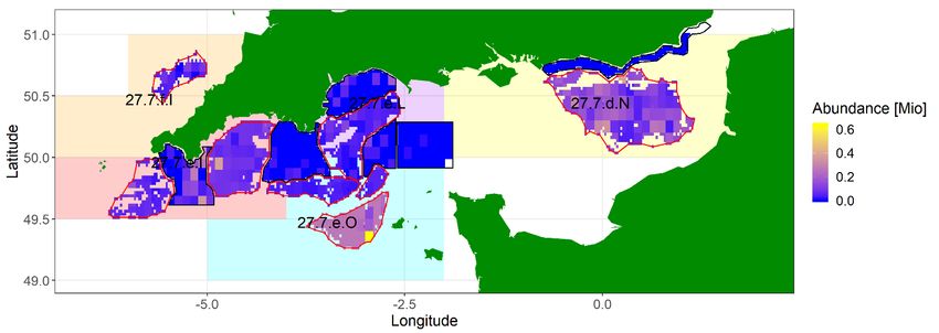
Table 6.1: Sampling summary from the 2018 dredge survey in Bed 7.d.2.

 Bed Number of Number of Number Number Aged
 Stations Length Measured
 Samples

 7.d.2 4 4 238 46

Figure 6.1: Sampled blocks in Bed 7.d.2 (Area 27.7.d.S) in 2018. Block shading indicates the
total number of stations within each block 0 =grey, 1=blue.

6.2. Raised biomass estimates and uncertainty
The estimated biomass of harvestable scallop (round shell length ≥ 110 mm, the MLS)
raised to each block is presented in Figure 6.2.

 24

Figure 6.2: Biomass of harvestable (round shell length ≥ 110 mm, the MLS) scallops in Bed
7.d.2 (Area 27.7.d.S) in 2018.

In order to estimate the uncertainty around harvestable biomass, the samples for each bed
were bootstrapped 5000 times with replacement. For each iteration, the same raising
procedure was used as for the main biomass estimation routine. The median, 25th and
75th percentiles and point estimates are given in Table 6.2.

 25

Table 6.2: Biomass estimate for Bed 7.d.2 based on the 2018 dredge survey.

 Bed 25th Percentile Median Point Estimate 75th Percentile
 (tonnes) Harvestable (tonnes) (tonnes)
 Biomass

 (tonnes)

 7.d.2 628 738 721 833

6.3. Size composition from dredge survey
From the size frequencies taken at each station, a total length frequency was pooled to the
total population estimate for Bed 7.d.2 (Figure 6.3).

Figure 6.3: Numbers (millions) per 5-mm length class for the scallop population in Bed 7.d.2
in 2018. The vertical line represents MLS.

6.4. Conclusion
This bed was defined following recent spatial expansion of fishing activity by both UK and
French fleets and is the first dredge survey undertaken for scallops in this bed. This bed is
positioned between Bed 7.d.1 (Area 27.7.d.N) in the north, and the Baie de Seine (Area
27.7.d.S) in the south, which is surveyed by IFREMER. There is scope for Area 27.7.d.S to
be internationally assessed.

 26

Only four tows were carried out in this small bed in 2018, and as such the biomass
estimates are only indicative.

A presentation of the assessment approach to the ICES Scallop Working Group
highlighted that there are several key areas of uncertainty that require further work to
better understand their impact. With the swept area biomass assessment, the key
parameter is the gear-efficiency estimate, and even relatively small changes to this
estimate would have a significant impact upon the estimated harvestable biomass and
harvest rate. Research to develop novel technology to resolve gear efficiency estimates
are still ongoing, as discussed above.

7. References
Edelsbrunner, H., Kirkpatrick, D. G. and Seidel, R. 1983. On the Shape of a Set of
Points in the Plane. IEEE Trans. Inform. Theory. 1983, Vol. 29, 4, pp. 551–559.

Nicolle, A., et al. 2017. Modelling larval dispersal of Pecten maximus in the English
Channel: a tool for the spatial management of the stocks. ICES Journal of Marine Science.
2017, Vol. 74, 6, pp. 1812-1825.

 27

World Class Science for the Marine and Freshwater Environment

We are the government’s marine and freshwater science experts. We help keep our seas,
oceans and rivers healthy and productive and our seafood safe and sustainable by
providing data and advice to the UK Government and our overseas partners. We are
passionate about what we do because our work helps tackle the serious global problems
of climate change, marine litter, over-fishing and pollution in support of the UK’s
commitments to a better future (for example the UN Sustainable Development Goals and
Defra’s 25 year Environment Plan).

We work in partnership with our colleagues in Defra and across UK government, and with
international governments, business, maritime and fishing industry, non-governmental
organisations, research institutes, universities, civil society and schools to collate and
share knowledge. Together we can understand and value our seas to secure a
sustainable blue future for us all, and help create a greater place for living.

© Crown copyright 2020

 __________________________________________________________________

 Pakefield Road, Lowestoft, Suffolk, NR33 0HT

 The Nothe, Barrack Road, Weymouth DT4 8UB

 www.cefas.co.uk | +44 (0) 1502 562244