Automatic Foreground Extraction from Imperfect Backgrounds using Multi-Agent Consensus Equilibrium
←
→
Page content transcription
If your browser does not render page correctly, please read the page content below
1
Automatic Foreground Extraction from Imperfect
Backgrounds using Multi-Agent Consensus
Equilibrium
Xiran Wang, Student Member, IEEE, Jason Juang and Stanley H. Chan, Senior Member, IEEE
Abstract—Extracting accurate foreground objects from a scene is an essential step for many video applications. Traditional
background subtraction algorithms can generate coarse estimates, but generating high quality masks requires professional softwares
with significant human interventions, e.g., providing trimaps or labeling key frames. We propose an automatic foreground extraction
arXiv:1808.08210v3 [cs.CV] 31 May 2020
method in applications where a static but imperfect background is available. Examples include filming and surveillance where the
background can be captured before the objects enter the scene or after they leave the scene. Our proposed method is very robust and
produces significantly better estimates than state-of-the-art background subtraction, video segmentation and alpha matting methods.
The key innovation of our method is a novel information fusion technique. The fusion framework allows us to integrate the individual
strengths of alpha matting, background subtraction and image denoising to produce an overall better estimate. Such integration is
particularly important when handling complex scenes with imperfect background. We show how the framework is developed, and how
the individual components are built. Extensive experiments and ablation studies are conducted to evaluate the proposed method.
Index Terms—Foreground extraction, alpha matting, video matting, Multi-Agent Consensus Equilibrium, background subtraction
F
1 I NTRODUCTION Using the plate image is significantly less expensive than
using the green screens. However, plate images are never
Extracting accurate foreground objects is an essential step
perfect. The proposed method is to robustly extract the
for many video applications in filming, surveillance, envi-
foreground masks in the presence of imperfect plate images.
ronment monitoring and video conferencing [1], [2], as well
as generating ground truth for performance evaluation [3].
As video technology improves, the volume and resolution of 1.1 Main Idea
the images have grown significantly over the past decades.
The proposed method, named Multi-Agent Consensus
Manual labeling has become increasingly difficult; even
Equilibrium (MACE), is illustrated in Figure 1. At the high
with the help of industry-grade production softwares, e.g.,
level, MACE is an information fusion framework where we
NUKE, producing high quality masks in large volume is still
construct a strong estimator from several weak estimators.
very time-consuming. The standard solution in the industry
By calling individual estimators as agents, we can imagine
has been chroma-keying [4] (i.e., using green screens). How-
that the agents are asserting forces to pull the information
ever, setting up green screens is largely limited to indoor
towards themselves. Because each agent is optimizing for
filming. When moving to outdoor, the cost and manpower
itself, the system is never stable. We therefore introduce a
associated with the hardware equipment is enormous, not
consensus agent which averages the individual signals and
to mention the uncertainty of the background lighting. In
broadcast the feedback information to the agents. When the
addition, some dynamic scenes prohibit the usage of green
individual agents receive the feedback, they adjust their
screens, e.g., capturing a moving car on a road. Even if
internal states in order to achieve an overall equilibrium.
we focus solely on indoor filming, green screens still have
The framework is theoretically guaranteed to find the equi-
limitations for 360-degree cameras where cameras are sur-
librium state under mild conditions.
rounding the object. In situations like these, it is unavoidable
In this paper, we present a novel design of the agents,
that the equipments become part of the background.
F1 , F2 , F3 . Each agent has a different task: Agent 1 is an
This paper presents an alternative solution for the afore-
alpha mating agent which takes the foreground background
mentioned foreground extraction task. Instead of using a
pair and try to estimate the mask using the alpha matting
green screen, we assume that we have captured the back-
equation. However, since alpha matting sometimes has false
ground image before the object enters or after it leaves the
alarms, we introduce Agent 2 which is a background esti-
scene. We call this background image as the plate image.
mation agent. Agent 2 provides better edge information and
X. Wang and S. Chan are with the School of Electrical and Computer
hence the mask. The last agent, Agent 3, is a denoising agent
Engineering, Purdue University, West Lafayette, IN 47907, USA. Email: { which promotes smoothness of the masks so that there will
wang470, stanchan}@purdue.edu. This work is supported, in part, not be isolated pixels.
by the National Science Foundation under grants CCF-1763896 and CCF- As shown in Figure 1, the collection of the agents is
1718007.
J. Juang is with HypeVR Inc., San Diego, CA 92108, USA. Email: the operator F which takes some signal and updates it.
jason@hypevr.com There is G which is the consensus agent. Its goal is to take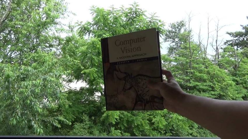
2

Fig. 1. Conceptual illustration of the proposed MACE framework. Given the input image and the background plate, the three MACE agents
individually computes their estimates. The consensus agent aggregates the information and feeds back to the agents to ask for updates. The
iteration continues until all the agents reach a consensus which is the final output.

averages of the incoming signals and broadcast the average            2     BACKGROUND
as a feedback. The red arrows represent signals flowing into          2.1    Related Work
the consensus agent, and the green arrows represent signals
flowing out to the individual agents. The iteration is given          Extracting foreground masks has a long history in computer
by the consensus equation. When the iteration terminates,             vision and image processing. Survey papers in the field
we obtain the final estimate.                                         are abundant, e.g., [8]–[10]. However, there is a subtle but
                                                                      important difference between the problem we are studying
                                                                      in this paper with the existing literature, as illustrated in
                                                                      Figure 2 and Table 1. At the high level, these differences
1.2   Contributions
                                                                      can be summarized in three forms: (1) Quality of the output
While most of the existing methods are based on developing            masks. (2) Requirement of the input (3) Automation and su-
a single estimator, this paper proposes to use a consensus            pervision. We briefly describe the comparison with existing
approach. The consensus approach has several advantages,              methods.
which correspond to the contributions of this paper.                  • Alpha Matting. Alpha matting is a supervised method.

  •   MACE is a training-free approach. We do not require               Given a user labeled “trimap”, the algorithm uses a
      training datasets like those deep learning approaches.            linear color model to predict the likelihood of a pixel
      MACE is an optimization-based approach. All steps                 being foreground or background as shown in Figure 2. A
      are transparent, explainable, interpretable, and can be           few better known examples include Poisson matting [11],
      debugged.                                                         closed-form matting [12], shared matting [13], Bayesian
  •   MACE is fully automatic. Unlike classical alpha matting           matting [14], and robust matting [15]. More recently, deep
      algorithms where users need to feed manual scribbles,             neural network based approaches are proposed, e.g., [16],
      MACE does not require human in the loop. As will be               [7], [17] and [18]. The biggest limitation of alpha matting
      shown in the experiments, MACE can handle a variety               is that the trimaps have to be error-free. As soon there is a
      of imaging conditions, motion, and scene content.                 false alarm of miss in the trimap, the resulting mask will
  •   MACE is guaranteed to converge under mild condi-                  be severely distorted. In video setting, methods such as
      tions which will be discussed in the theory section of            [19]–[21] suffer similar issues of error-prone trimaps due
      this paper.                                                       to temporal propagation. Two-stage methods such as [22]
  •   MACE is flexible. While we propose three specific                 requires initial segmentation [23] to provide the trimap
      agents for this problem and we have shown their ne-               and suffer the same problem. Other methods [24], [25]
      cessity in the ablation study, the number and the type            require additional sensor data, e.g., depth, which is not
      of agents can be expanded. In particular, it is possible          always available.
      to use deep learning methods as agents in the MACE              •   Background Subtraction. Background subtraction is un-
      framework.                                                          supervised. Existing background subtraction methods
  •   MACE offers the most robust result according to the                 range from the simple frame difference method to the
      experiments conducted in this paper. We attribute this              more sophisticated mixture models [26], contour saliency
      to the complementarity of the agents when handling                  [27], dynamic texture [28], feedback models [5] and at-
      difficult situations.                                               tempts to unify several approaches [29]. Most background
   In order to evaluate the proposed method, we have                      subtraction methods are used to track objects instead of
compared against more than 10 state-of-the-art video seg-                 extracting the alpha mattes. They are fully-automated and
mentation and background subtraction methods, including                   are real time, but the foreground masks generated are
several deep neural network solutions. We have created a                  usually of low quality.
database with ground truth masks and background images.                   It is also important to mention that there work about
The database will be release to the general public on our                 initializing the background image. These methods are
project website. We have conducted an extensive ablation                  particularly useful when the pure background plate image
study to evaluate the importance of individual components.                is not available. Bouwmans et al. has a comprehensive
3

Fig. 2. The landscape of the related problems. We group the methods according to the level of supervision they need during the inference stage.
Background Subtraction (e.g., [5]) aims at locating objects in a video, and most of the available methods are un-supervised. Video Segmentation
(e.g., [6]) aims at identifying the salient objects. The training stage is supervised, but the inference stage is mostly un-supervised. Alpha matting
(e.g., [7]) needs a high-quality trimap to refine the uncertain regions of the boundaries, making it a supervised method. Our proposed method is in
the middle. We do not need a high-quality trimap but we assume an imperfect background image.

                              TABLE 1                                           We emphasize that the problem we study in this paper
  Objective and Assumptions of (a) Alpha matting, (b) Background            does not belong to any of the above categories. Existing
Subtraction, (c) Unsupervised Video Segmentation, and (d) Our work.
                                                                            alpha matting algorithms have not been able to handle
                                                                            imperfect plate images, whereas background subtraction is
    Method       Alpha         Bkgnd         Video         Ours
                 Matting     Subtraction   Segmentation                     targeting a completely different objective. Saliency based
    Goal       foreground      object       saliency    foreground          unsupervised video segmentation is an overkill, in particu-
               estimation     detection     detection   estimation
                                                                            lar those deep neural network solutions. More importantly,
    Input      image+trimap    video         video      image+plate
    Accuracy      high      low (binary)    medium         high             currently there is no training sets for plate image. This
    Automatic     semi           full          full         full            makes learning-based methods impossible. In contrast, the
    Supervised    semi            no            no         semi
                                                                            proposed method does not require training. Note that the
                                                                            plate image assumption in our work is the practical reality
    survey about the approaches [30]. In addition, a number                 for many video applications. The problem remains challeng-
    of methods should be noted, e.g., [31]–[36].                            ing because the plate images are imperfect.

• Unsupervised Video Segmentation. Unsupervised video
                                                                            2.2   Challenges of Imperfect Background
  segmentation, as it is named, is unsupervised and fully
  automatic. The idea is to use different saliency cues                     Before we discuss the proposed method, we should explain
  to identify objects in the video, and then segments                       the difficulty of an imperfect plate. If the plate were perfect
  them out. Early approaches include key-segments [37],                     (i.e., static and matches perfectly with the target images),
  graph model [38], contrast based saliency [39], motion                    then a standard frame difference with morphographic oper-
  cues [40], non-local statistics [41], co-segmentation [42],               ations (e.g., erosion / dilation) would be enough to provide
  convex-optimization [43]. State-of-the-art video segmen-                  a trimap, and thus a sufficiently powerful alpha matting
  tation methods are based on deep neural networks, such                    algorithm would work. When the plate image is imperfect,
  as using short connection [44], pyramid dilated networks                  then complication arises because the frame difference will
  [45], super-trajectory [46], video attention [6], and feature             be heavily corrupted.
  pyramid [47], [48]. Readers interested in the latest devel-                    The imperfectness of the plate images comes from one
  opments of video segmentation can consult the tutorial                    or more of the following sources:
  by Wang et al. [49]. Online tools for video segmentation                  • Background vibration. While we assume that the plate
  are also available [50]. One thing to note is that most of                   does not contain large moving objects, small vibration of
  the deep neural network solutions require post-processing                    the background generally exists. Figure 3 Case I shows an
  methods such as conditional random field [51] to fine                        example where the background tree vibrates.
  tune the masks. If we directly use the network output,                    • Color similarity. When foreground color is very similar to
  the results are indeed not good. In contrast, our method                     the background color, the trimap generated will have false
  does not require any post-processing.                                        alarms and misses. Figure 3 Case II shows an example
    Besides the above mentioned papers, there are some                         where the cloth of the man has a similar color to the wall.
existing methods using the consensus approach, e.g., the                    • Auto-exposure. If auto-exposure is used, the background
early work of Wang and Suter [52], Han et al. [53], and more                   intensity will change over time. Figure 3 Case III shows an
recently the work of St. Charles et al. [54]. However, the                     example where the background cabinet becomes dimmer
notion of consensus in these papers are more about making                      when the man leaves the room.
votes for the mask. Our approach, on the other hand, are                         As shown in the examples, error in frame difference
focusing on information exchange across agents. Thus, we                    can be easily translated to false alarms and misses in the
are able to offer theoretical guarantees whereas the existing               trimap. While we can increase the uncertainty region of the
consensus approaches are largely rule-based heuristics.                     trimap to rely more on the color constancy model of the
4

       I

      II

      III
                  (a) Input          (b) Plate         (c) Frame diff.          (d) Trimap           (e) DCNN               (f) Ours
Fig. 3. Three common issues of automatic foreground extraction. Case I: Vibrating background. Notice the small vibration of the leaves in the
background. Case II. Similar foreground / background color. Notice the missing parts of the body of the man, and the excessive large uncertainty
region of the trimap. Case III. Auto-exposure. Notice the false alarm in the background of the frame difference map. We compare our method with
DCNN [7], a semi-supervised alpha matting method using the generated trimaps. The video data of Case III is from [55].

alpha matting, in general the alpha matting performs worse               a prior distribution of the latent image. ADMM solves the
when the uncertainty region grows. We have also tested                   problem by solving a sequence of subproblems as follows:
more advanced background estimation algorithms, e.g., [5]
in OpenCV. However, the results are similar or sometimes                     (k+1)                    ρ       (k)
                                                                           x1        = argmin f1 (v) + kv − (x2 − u(k) )k2 ,     (2a)
even worse. Figure 4 shows a comparison using various                                   v∈R n         2
alpha matting algorithms.                                                    (k+1)                    ρ       (k+1)
                                                                           x2        = argmin f2 (v) + kv − (x1     + u(k) )k2 , (2b)
                                                                                        v∈R n         2
                                                                                                  (k+1)      (k+1)
3     M ULTI -AGENT C ONSENSUS E QUILIBRIUM                                u(k+1) = u(k) + (x1            − x2       ).                    (2c)

Our proposed method is an information fusion technique.                  In the last equation (2c), the vector u(k) ∈ Rn is the
The motivation for adopting a fusion strategy is that for                Lagrange multiplier associated with the constraint. Under
complex scenarios, no single estimator can be uniformly                  mild conditions, e.g., when f1 and f2 are convex, close, and
superior in all situations. Integrating weak estimators to               proper, global convergence of the algorithm can be proved
construct a stronger one is likely more robust and can                   [62]. Recent studies show that ADMM converges even for
handle more cases. The weak estimators we use in this paper              some non-convex functions [63].
are the alpha matting, background subtraction and image
                                                                             When f1 and f2 are convex, the minimizations in (2a)
denoising. We present a principled method to integrate
                                                                         and (2b) are known as the proximal maps of f1 and f2 ,
these estimators.
                                                                         respectively [64]. If we define the proximal maps as
     The proposed fusion technique is based on the Multi-
Agent Consensus Equilibrium (MACE), recently developed                                                         ρ
by Buzzard et al. [60]. Recall the overview diagram shown                              Fi (z) = argmin fi (v) + kv − zk2 ,                  (3)
                                                                                                 v∈R n         2
in Figure 1. The method consists of three individual agents
which perform specific tasks related to our problem. The                 then it is not difficult to see that at the optimal point, (2a)
agents will output an estimate based on their best knowl-                and (2b) become
edge and their current state. The information is aggregated
by the consensus agents and broadcast back to the individ-                                       F1 (x∗ − u∗ ) = x∗ ,                      (4a)
ual agents. The individual agents update their estimates un-                                     F2 (x∗ + u∗ ) = x∗ ,                      (4b)
til all three reaches a consensus which is the final output. We
will discuss the general principle of MACE in this section,              where (x∗ , u∗ ) are the solutions to the original constrained
and describe the individual agents in the next section.                  optimization in (1). (4a) and (4b) shows that the solution
                                                                         (x∗ , u∗ ) can now be considered as a fixed point of the
3.1        ADMM                                                          system of equations.
The starting point of MACE is the alternating direction                      Rewriting (2a)-(2c) in terms of (4a) and (4b) allows us
method of multipliers (ADMM) algorithm [61]. The ADMM                    to consider agents Fi that are not necessarily proximal
algorithm aims at solving a constrained minimization:                    maps, i.e., fi is not convex or Fi may not be expressible as
                                                                         optimizations. One example is to use an off-the-shelf image
    minimize f1 (x1 ) + f2 (x2 ),     subject to     x1 = x2 ,     (1)   denoiser for Fi , e.g., BM3D, non-local means, or neural
       x1 ,x2
                                                                         network denoisers. Such algorithm is known as the Plug-
where xi ∈ Rn , and fi : Rn → R are mappings, typically a                and-Play ADMM [62], [63], [65] (and variations thereafter
forward model describing the image formation process and                 [60], [66]).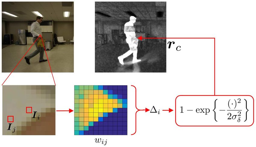
5
(a) Input (b) Frame difference (c) Trimap (d) Closed-form (e) Spectral matting
matting [12] [56]
(f) Learning-based (g) K-nearest (h) Comprehensive (i) DCNN [7] (j) Ours
matting [57] neighbors [58] sampling [59] (without trimap)
Fig. 4. Comparison with existing alpha-matting algorithms on real images with a frame-difference based trimap. (a) Input image. (b) Frame
difference. (c) Trimap generated by morphographic operation (dilation / erosion) of the binary mask. (d) - (i) Alpha matting algorithms available
on alphamatting.com. (j) Proposed method. This sequence is from the dataset of [55].
def 1 PN
3.2 MACE and Intuition where hzi = N i=1 z i is the average of z .
MACE generalizes the above ADMM formulation. Instead
of minimizing a sum of two functions, MACE minimizes a Algorithm 1 MACE Algorithm
sum of N functions f1 , . . . , fN :
1: Initialize v t = [v t1 , . . . , v tN ].
N
X 2: for t = 1, . . . , T do
minimize fi (xi ), x1 = . . . = xN . (5) 3: % Perform agent updates, (2F − I)(v t )
x1 ,...,xN
i=1
4:
z t1 2F1 (v t1 ) − v t1
In this case, the equations in (4a)-(4b) are generalized to
.. ..
. = (10)
Fi (x∗ + u∗i ) = x∗ , for i = 1, . . . , N .
PN ∗ (6) zNt t
2FN (v N ) − v N t
i=1 ui = 0.
What does (6) buy us? Intuitively, (6) suggests that in a 5:
system containing N agents, each agent will create a tension 6: % Perform the data aggregation (2G − I)(z t )
u∗i ∈ Rn . For example, if F1 is an inversion step whereas F2 7: t+1
2hz t i − z t1
v1
is a denoising step, then F1 will not agree with F2 because .. ..
. = (11)
F1 tends to recover details but F2 tends to smooth out .
t t
details. The agents F1 , . . . , FN will reach an equilibrium v t+1
N
2hz i − z N
state where the sum of the tension is zero. This explains
8: end for
the name “consensus equilibrium”, as the the algorithm is
9: Output hv T i.
seeking a consensus among all the agents.
How does the equilibrium solution look like? The fol-
lowing theorem, shown in [60], provides a way to connect Theorem 1 provides a full characterization of the MACE
the equilibrium condition to a fixed point of an iterative solution. The operator G in Theorem 1 is a consensus agent
algorithm. that takes a set of inputs z 1 , . . . , z N and maps them to
their average hzi. In fact, we can show that G is a projec-
def
Theorem 1 (MACE solution [60]). Let u∗ = [u∗1 ; . . . ; u∗N ]. tion and that (2G − I) is its self-inverse [60]. As a result,
The consensus equilibrium (x∗ , u∗ ) is a solution to the MACE (8) is equivalent to (2F − I)v ∗ = (2G − I)v ∗ . That is,
def we want the individual agents F1 , . . . , FN to match with
equation (6) if and only if the points v ∗i = x∗ + u∗i satisfy
the consensus agent G such that the equilibrium holds:
N
1 X ∗ (2F − I)v ∗ = (2G − I)v ∗ .
v = x∗ (7)
N i=1 i The algorithm of the MACE is illustrated in Algorithm 1.
According to (8), v ∗ is a fixed point of the set of equilibrium
(2G − I)(2F − I)v ∗ = v ∗ , (8) equations. Finding the fixed point can be done by iteratively
def updating v (t) through the procedure
where v ∗ = [v ∗1 ; . . . ; v ∗N ] ∈ RnN , and F, G : RnN → RnN are
mappings defined as v (t+1) = (2G − I)(2F − I)v (t) . (12)
hzi
F1 (z 1 ) Therefore, the algorithmic steps are no more complicated
F(z) = .. , G(z) =
..
and . , (9) than updating the individual agents (2F − I) in parallel,
.
FN (z N ) hzi and then aggregating the results through (2G − I).
6
The convergence of MACE is guaranteed when T is non- have alpha matte αI for I , and the alpha matte αP for P .
expansive [60]summarized in the proposition below. When P is given, we can redefine the color line model as
def
I c
Proposition 1. Let F and G be defined as (9), and let T = αi X
c Ii
≈ a + b. (17)
(2G − I)(2F − I). Then the following results hold: αiP Pic
c∈{r,g,b}
(i) F is firmly non-expansive if all Fi ’s are firmly non-
expansive. In other words, we ask the coefficients (ar , ag , ab , b) to fit
(ii) G is firmly non-expansive. simultaneously the actual image I and the plate image
(iii) T is non-expansive if F and G are firmly non-expansive. P . When (17) is assumed, the energy function J(α, a, b)
becomes
Proof. See Appendix. ( !2
X X X
I P I c c
J(α , α , a, b) =
e α − a I − bji j i
j∈I i∈wj c
4 D ESIGNING MACE AGENTS !2 )
After describing the MACE framework, in this section we X X X
+η αiP − acj Pic − bj + (acj )2 , (18)
discuss how each agent is designed for our problem. i∈wj c c
where we added a constant η to regulate the relative em-
4.1 Agent 1: Dual-Layer Closed-Form Matting
phasis between I and P .
The first agent we use in MACE is a modified version of the
classic closed-form matting. More precisely, we define the Theorem 2. The marginal energy function
agent as def
J(α)
e = min J(α,
e 0, a, b) (19)
T a,b
e + λ1 (α − z)T D(α
F1 (z) = argmin α Lα f − z), (13)
α can be equivalently expressed as J(α)
e = αT Lαe , where L e ∈
n×n
where L
e and D f are matrices, and will be explained below. R is the modified matting Laplacian, with the (i, j)th element
The constant λ1 is a parameter.
(
X 1
Li,j =
e δij − 1 + (I i − µk )T
Review of Closed-Form Matting. To understand the mean- 2|wk |
k|(i,j)∈wk
ing of (13), we recall that the classical closed-form matting −1
!)
is an algorithm that tries to solve Σk − n(1 + η)µk µk T
(I j − µk ) . (20)
J(α, a, b)
!2 Here, δij is the Kronecker delta, I i ∈ R3 is the color vector at the
ith pixel. The vector µk ∈ R3 is defined as
X X X X
= αi − acj Iic − bj + (acj )2 . (14)
j∈I i∈wj c c 1 X
µk = (I j + P j ), (21)
Here, (ar , ag , ab , b) are the linear 2|wk | j∈w
P combinationc c
coefficients k
of the color line model αi ≈ c∈{r,g,b} a Ii + b, and αi 3×3
and the matrix Σk ∈ R is
is the alpha matte value of the ith pixel [12]. The weight (
wj is a 3 × 3 window of pixel j . With some algebra, we 1 1 X
def Σk = (I j − µk )(I j − µk )T
can show that the marginalized energy function J(α) = 2 |wk | j∈w
k
mina,b J(α, a, b) is equivalent to )
1 X T
def
J(α) = min J(α, a, b) = αT Lα, (15)
+ (P j − µk )(P j − µk ) . (22)
a,b
|wk | j∈w
k
where L ∈ Rn×n is the so-called matting Laplacian matrix. Proof. See Appendix.
When trimap is given, we can regularize J(α) by minimiz- Because of the plate term in (18), the modified matting
ing the overall energy function:
Laplacian L
e is positive definite. See Appendix for proof. The
b = argmin αT Lα + λ(α − z)T D(α − z),
α (16) original L in (15) is only positive semi-definite.
α
where D is a binary diagonal matrix with entries being one Dual-Layer Regularization D f. The diagonal regularization
for pixels that are labeled in the trimap, and zero otherwise. matrix Df in (13) is reminiscent to the binary matrix D in
The vector z ∈ Rn contains specified alpha values given (16), but D f is defined through a sigmoid function applied
by the trimap. Thus, for large λ, the minimization in (16) f def
to the input z . To be more precise, we define D = diag(dei ),
will force the solution to satisfy the constraints given by the where
trimap.
1
dei = diag ∈ Rn×n , (23)
Dual-Layer Matting Laplacian L e . In the presence of the 1 + exp{−κ(zi − θ)}
plate image, we have two pieces of complementary informa- and zi is the i-th element of the vector z ∈ Rn , which is the
tion: I ∈ Rn×3 the color image containing the foreground argument of F1 . The scalar constant κ > 0 is a user defined
object, and P ∈ Rn×3 the plate image. Correspondingly, we parameter specifying the stiffness of the sigmoid function,
7

and 0 < θ < 1 is another user defined parameter specifying
the center of the transient. Typical values of (κ, θ) for our
MACE framework are κ = 30 and θ = 0.8.
   A closer inspection of D and D  f reveals that D is per-
forming a hard-threshold whereas D   f is performing a soft-
                                   def
threshold. In fact, the matrix D = diag(di ) has diagonal
entries               (
                        0,    θ1 < zi < θ2 ,
                 di =                                     (24)
                        1,    otherwise.
for two cutoff values θ1 and θ2 . This hard-threshold is
equivalent to the soft-threshold in (23) when κ → ∞.
    There are a few reasons why (23) is preferred over
(24), especially when we have the plate image. First, the         Fig. 5. Illustration of how to construct the estimate r c . We compute the
soft-threshold in (23) tolerates more error present in z ,        distance between the foreground and the background. The distance has
                                                                  a bilateral weight to improve robustness. The actual r 0 represents the
because the values of Df represent the probability of having
                                                                  probability of having a foreground pixel.
foreground pixels. Second, the one-sided threshold in (23)
ensures that the background portion of the image is handled
by the plate image rather than the input z . This is usually      where
beneficial when the plate is reasonably accurate.
                                                                                 kxi − xj k2           kI i − I j k2

                                                                     eij = exp −
                                                                     w                         exp   −                 .               (29)
4.2   Agent 2: Background Estimator                                                  2h2s                   2h2r
Our second agent is a background estimator, defined as            Here, xi denotes the spatial coordinate of pixel i, I i ∈ R3
                                                                  denotes the ith color pixel of the color image I , and (hs , hr )
F2 (z) = argmin kα − r 0 k2 + λ2 kα − zk2 + γαT (1 − α).
            α                                                     are the parameters controlling the bilateral weight strength.
                                                          (25)    The typical values of hs and hr are both 5.
The reason of introducing F2 is that in F1 , the matrix Df is
                                                                     We now need a mapping which maps the distance ∆ =
                                                                                                                                         def

determined by the current estimate z . While Df handles part
                                                                  [∆1 , . . . , ∆n ]T to a vector of numbers r c in [0, 1]n so that
of the error in z , large missing pixels and false alarms can     the term kα − r 0 k2 makes sense. To this end, we choose a
still cause problems especially in the interior regions. The      simple Gaussian function:
goal of F2 is to complement F1 for these interior regions.                                            (     )
                                                                                                        ∆2
Initial Background Estimate r 0 . Let us take a look at (25).                            r c = 1 − exp − 2 ,                   (30)
                                                                                                        2σδ
The first two terms are quadratic. The interpretation is that
given some fixed initial estimate r 0 and the current input z ,   where σδ is a user tunable parameter. We tested other
F2 (z) returns a linearly combined estimate between r 0 and       possible mappings such as the sigmoid function and the
z . The initial estimate r 0 consists of two parts:               cumulative distribution function of a Gaussian. However,
                        r0 = rc    re ,                    (26)   we do not see significant difference compared to (30). The
                                                                  typical value for σδ is 10.
where      means elementwise multiplication. The first term
r c is the color term, measuring the similarity between fore-     Defining the Edge Term r e . The color term r c is able
ground and background colors. The second term r e is the          to capture most of the difference between the image and
edge term, measuring the likelihood of foreground edges           the plate. However, it also generates false alarms if there
relative background edges. In the followings we will discuss      is illumination change. For example, shadow due to the
these two terms one by one.                                       foreground object is often falsely labeled as foreground. See
                                                                  the shadow near the foot in Figure 5.
Defining the Color Term P r c . We define r c by measuring the        In order to reduce the false alarm due to minor illu-
distance kI j −P j k2 = c∈{r,g,b} (Ijc −Pjc )2 between a color    mination change, we first create a “super-pixel” mask by
pixel I j ∈ R3 and a plate pixel P j ∈ R3 . Ideally, we would     grouping similar colors. Our super-pixels are generated by
like r c to be small when kI j − P j k2 is large.                 applying a standard flood-fill algorithm [67] to the image I .
    In order to improve the robustness of kI j −P j k2 against    This gives us a partition of the image I as
noise and illumination fluctuation, we modify kI j − P j k2
by using the bilateral weighted average over a small neigh-                            I → {I S1 , I S2 , . . . , I Sm },              (31)
borhood:
                                                                  where S1 , . . . , Sm are the m super-pixel index sets. The plate
                        X
                  ∆i =      wij kI j − P j k2 ,           (27)
                       j∈Ωi                                       image is partition using the same super-pixel indices, i.e.,
                                                                  P → {P S1 , P S2 , . . . , P Sm }.
where Ωi specifies a small window around the pixel i. The
                                                                     While we are generating the super-pixels, we also com-
bilateral weight wij is defined as
                                                                  pute the gradients of I and P for every pixel i = 1, . . . , n.
                              w
                              eij                                 Specifically, we define ∇I i = [∇x I i , ∇y I i ]T and ∇P i =
                       wij = P      ,                      (28)
                              jweij                               [∇x P i , ∇y P i ]T , where ∇x I i ∈ R3 (and ∇y I i ∈ R3 ) are the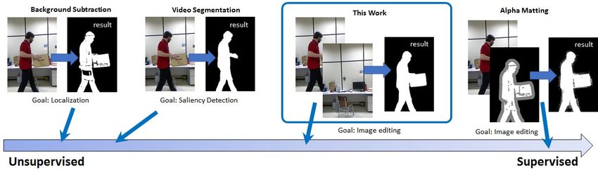
8

                                                                               effect of this term can be seen from the fact that αT (1 − α)
                                                                               is a symmetric concave quadratic function with a value zero
                                                                               for α = 1 or α = 0. Therefore, it introduces penalty for
                                                                               solutions that are away from 0 or 1. For γ ≤ 1, one can show
                                                                               that the Hessian matrix of the function f2 (α) = kα−r 0 k2 +
                                                                               γαT (1 − α) is positive semidefinite. Thus, f2 is strongly
                                                                               convex with parameter γ .

                                                                               4.3 Agent 3: Total Variation Denoising
                                                                               The third agent we use in this paper is the total variation
                                                                               denoising:
                                                                                          F3 (z) = argmin kαkTV + λ3 kα − zk2 ,                (35)
                                                                                                       α
Fig. 6. Illustration of how to construct the estimate r e .                    where λ3 is a parameter. The norm k · kTV is defined in
                                                                               space-time:
                                                                                        def
                                                                                            Xq
                                                                                 kvkTV =       βx (∇x v)2 + βy (∇y v)2 + βt (∇t v)2 , (36)
                                                                                             i,j,t

                                                                               where (βx , βy , βt ) controls the relative strength of the gradi-
                                                                               ent in each direction. In this paper, for spatial total variation
                                                                               we set (βx , βy , βt ) = (1, 1, 0), and for spatial-temporal total
                                                                               variation we set (βx , βy , βt ) = (1, 1, 0.25).
           (a) r c                  (b) r e                   (c) r 0
                                                                                  A denoising agent is used in the MACE framework be-
Fig. 7. Comparison between r c , r e , and r 0 .                               cause we want to ensure smoothness of the resulting matte.
                                                                               The choice of the total variation denoising operation is a
two-tap horizontal (and vertical) finite difference at the i-th                balance betweeen complexity and performance. Users can
pixel. To measure how far I i is from P i , we compute                         use stronger denoisers such as BM3D. However, these patch
                          θi = k∇I i − ∇P i k2 .                        (32)   based image denoising algorithms rely on the patch match-
                                                                               ing procedure, and so they tend to under-smooth repeated
Thus, θi is small for background regions because I i ≈ P i ,                   patterns of false alarm / misses. Neural network denoisers
but is large when there is a foreground pixel in I i . If we set               are better candidates but they need to be trained with the
a threshold operation after θi , i.e., set θi = 1 if θi > τθ for               specifically distorted alpha mattes. From our experience, we
some threshold τθ , then shadows can be removed as their                       do not see any particular advantage of using CNN-based
gradients are weak.                                                            denoisers. Figure 8 shows some comparison.
    Now that we have computed θi , we still need to map it
back to a quantity similar to the alpha matte. To this end,
we compute a normalization term
                     Ai = max (k∇I i k2 , k∇P i k2 ) ,                  (33)
and normalize 1{θi > τθ } by

                    j∈Si 1{Ai > τA }1{θi > τθ }
                   P
               def
        (re )i =                                ,                       (34)
                          j∈Si 1{Ai > τA }
                       P

where 1 denotes the indicator function, and τA and τθ are
thresholds. In essence, (34) says in the i-th super-pixel Si ,                       (a) Input       (b) TV         (c) BM3D        (d) IRCNN
we count the number of edges 1{θi > τθ } that have strong                                             [68]              [69]            [70]
difference between I i and P i . However, we do not want
                                                                               Fig. 8. Comparison of different denoisers used in MACE. Shown are the
to count every pixel but only pixels that already contains                     results when MACE converges. The shadow near the foot is a typical
strong edges, either in I or P . Thus, we take the weighted                    place of false alarm, and many denoisers cannot handle.
average using 1{Ai > τA } as the weight. This defines r e , as
                                                                               4.4    Parameters and Runtime
the weighted average (re )i is shared among all pixels in the
super-pixel Si . Figure 6 shows a pictorial illustration.                      The typical values for parameters of the proposed method
    Why is r e helpful? If we look at r c and r e in Figure 7,                 are presented in Table 4.4. λ1 and λ2 are rarely changed,
we see that the foreground pixels of r c and r e coincide but                  while λ3 determines the denoising strength of Agent 3. γ
background pixels roughly cancel each other. The reason is                     has a default value of 0.05. Inceasing γ causes more binary
that while r c creates weak holes in the foreground, r e fills                 results with clearer boundaries. τA and τθ determine the
the gap by ensuring the foreground is marked.                                  edge term r e in Agent 2 and are fixed. σδ determines the
                                                                               color term r c in Agent 2. Large σδ produces less false
Regularization αT (1 − α). The last term αT (1 − α) in (25)                    negative but more false positive. Overall, the performance
is a regularization to force the solution to either 0 or 1. The                is reasonably stable to these parameters.
9
TABLE 2
Typical values for parameters indicates the presence of shadow. Lighting issues in-
clude illumination change due to auto-exposure and auto-
Parameter λ1 λ2 λ3 γ τA τθ σδ white-balance. The background vibration only applies
Value 0.01 2 4 0.05 0.01 0.02 10 to outdoor scenes where the background objects have mi-
nor movements, e.g., moving grass or tree branches. The
In terms of runtime, the most time-consuming part is
camouflage column indicates the similarity in color be-
Agent 1 because we need to solve a large-scale sparse
tween the foreground and background, which is a common
least squares problem. Its runtime is determined by the
problem for most sequences. The green screen column
number of foreground pixels. Table 3 shows the runtime
shows which of the sequences have green screens to mimic
of the sequences we tested. In generating these results, we
the common chroma-keying environment.
used an un-optimized MATLAB code on a Intel i7-4770k.
The typical runtime is about 1-3 minutes per frame. From
our experience working with professional artists, even with 5.2 Competing methods
professional film production software, e.g., NUKE, it takes We categorize the competing methods into four different
15 minutes to label a ground truth label using the plate groups. The key ideas are summarized in Table 5.2.
and temporal cues. Therefore, the runtime benefit offered
by our algorithm is substantial. The current runtime can be • Video Segmentation: We consider four unsupervised
significantly improved by using multi-core CPU or GPU. video segmentation methods: Visual attention (AGS)
Our latest implementation on GPU achieves 5 seconds per [6], pyramid dilated bidirectional ConvLSTM (PDB)
frame for images of size 1280 × 720. [45], motion adaptive object segmentation (MOA) [50],
non-local consensus voting (NLVS) [41]. These methods
are fully-automatic and do not require a plate image.
5 E XPERIMENTAL R ESULTS All algorithms are downloaded from the author’s web-
5.1 Dataset sites and are run under default configurations.
• Background Subtraction: We consider two background
To evaluate the proposed method, we create a Purdue
subtraction algorithms Pixel-based adaptive segmenter
dataset containing 8 video sequences using the HypeVR
(PBAS) [5], Visual background extractor (ViBe) [29].
Inc. 360 degree camera. The original image resolution is
Both algorithms are downloaded from the author’s
8192 × 4320 at a frame rate of 48fps, and these images are
websites and are run under default configurations.
then downsampled and cropped to speed up the matting
• Alpha matting: We consider one of the state-of-the-art
process. In addition to these videos, we also include 6 videos
alpha matting algorithm using CNN [7]. The trimaps
sequences from a public dataset [55], making a total of 14
are generated by applying frame difference between the
video sequences. Snapshots of the sequences are shown in
plate and color images, followed by morphological and
Figure 9. All video sequences are captured without camera
thresholding operations.
motion. Plate images are available, either during the first
• Others: We consider the bilateral space video segmen-
or the last few frames of the video. To enable objective
tation (BSVS) [19] which is a semi-supervised method.
evaluation, for each video sequence we randomly select
It requires the user to provide ground truth labels for
10 frames and manually generate the ground truths. Thus
key frames. We also modified the original Grabcut [23]
totally there are 140 frames with ground truths.
to use the plate image instead of asking for user input.
5.3 Metrics
Building Coach Studio Road Tackle Gravel Office Book
The following four metrics are used.
(a) Snapshots of the Purdue Dataset
• Intersection-ver-union (IoU) measures the overlap be-
tween the estimate mask and the ground truth mask:
Bootstrap Cespatx Dcam
P
min (x
bi , xi )
Gen MP Shadow
(b) Snapshots of a public dataset [55] IoU = P i ,
i max (xbi , xi )
Fig. 9. Snapshots of the videos we use in the experiment. Top row: where x bi is the i-pixel of the estimated alpha matte, and xi
Building, Coach, Studio, Road, Tackle, Gravel, Office, Book. Bottom
row:Bootstrap, Cespatx, Dcam, Gen, MP, Shadow. is that of the ground truth. Higher IoU score is better.
• Mean-absolute-error (MAE) measures the average abso-
The characteristics of the dataset is summarized in Ta- lute difference between the ground truth and the estimate.
ble 3. The Purdue dataset has various resolution, and the Lower MAE is better.
Public dataset has one resolution 480 × 640. The fore- • Contour accuracy (F) [72] measures the performance from
ground percentage for the Purdue dataset videos ranges a contour based perspective. Higher F score is better.
from 1.03% to 55.10%, whereas that public dataset has • Structure measure (S) [73] simultaneously evaluates
similar foreground percentage around 10%. The runtime region-aware and object-aware structural similarity between
of the algorithm (per frame) is determined by the resolu- the result and the ground truth. Higher S score is better.
tion and the foreground percentage. In terms of content, • Temporal instability (T) [72] that performs contour
the Purdue dataset focuses on outdoor scenes whereas matching with polygon representations between two adja-
the public dataset are only indoor. The shadow column cent frames. Lower T score is better.
10

                                                                   TABLE 3
                                         Description of the video sequences used in our experiments.

                                                   time/Fr    indoor/                lighting   Backgrd                      green     ground
                          resolution     FGD %       (sec)    outdoor    shadow       issues    vibration    camouflage      screen     truth
               Book         540x960      19.75%       231     outdoor                               X            X                        X
            Building       632x1012       4.03%      170.8    outdoor       X                       X            X                        X
              Coach        790x1264       4.68%      396.1    outdoor                               X                          X          X
 Purdue       Studio        480x270      55.10%       58.3     indoor                                                                     X
 Dataset       Road        675x1175       1.03%      232.9    outdoor       X                      X             X                        X
              Tackle       501x1676       4.80%      210.1    outdoor       X                      X                           X          X
              Gravel       790x1536       2.53%      280.1    outdoor       X                      X             X                        X
              Office       623x1229       3.47%      185.3     indoor       X                                    X                        X
            Bootstrap       480x640      13.28%      109.1     indoor       X           X                        X                        X
             Cespatx        480x640      10.31%      106.4     indoor       X           X                        X                        X
 Public       DCam          480x640      12.23%      123.6     indoor       X           X                        X                        X
 Dataset       Gen          480x640      10.23%      100.4     indoor       X           X                        X                        X
  [55]     Multipeople      480x640       9.04%       99.5     indoor       X           X                        X                        X
             Shadow         480x640      11.97%      115.2     indoor       X           X                                                 X

                                                                   TABLE 4
                                                   Description of the competing methods.
                                                   Methods              Supervised          Key idea
                                                    NLVS        [41]       no           non-local voting
                                Unsupervised
                                                    AGS          [6]       no            visual attention
                                   Video
                                                    MOA         [50]       no         2-stream adaptation
                                Segmentation
                                                    PDB         [45]       no         pyramid ConvLSTM
                                   Alpha                                               Trimap generation
                                                   Matting     [71]      trimap
                                   matting                                              + alpha matting
                                 Background         ViBe        [29]       no          pixel model based
                                 subtraction        PBAS         [5]       no            non-parametric
                                                    BSVS        [19]    key frame        bilateral space
                                       Other
                                                   Grabcut      [23]      plate       iterative graph cuts

5.4   Results

• Comparison with video segmentation methods: The
results are shown in Table 5.4, where we list the average
IoU, MAE, F, S and T scores over the datasets. In this
table, we notice that the deep-learning solutions AGS [6],
MOA [50] and PDB [45] are significantly better than classical
optical flow based NLVS [41] in all the metrics. However,
since the deep-learning solutions are targeting for saliency
detection, foreground but unsalient objects will be missed.                     (a) Image        (b) AGS [6], before   (c) PDB [45], before
AGS performs the best among the three with a F measure of
0.91, S measure of 0.94 and T measure of 0.19. PDB performs
better than MOA in most metrics other than the T measure,
with PDB scoring 0.2 while MOA scoreing 0.19.
    We should also comment on the reliance on conditional
random field of these deep learning solutions. In Figure 10
we show the raw outputs of AGS [6] and PDB [45]. While
the salient object is correctly identified, the masks are coarse.
Only after the conditional random field [51] the results
become significantly better. In contrast, the raw output of
                                                                                (d) Ours          (e) AGS [6], after      (f) PDB [45], after
our proposed algorithm is already high quality.
                                                                        Fig. 10. Dependency of conditional random field. (a) Input. (b) Raw
• Comparison with trimap + alpha-matting methods: In                    output of the neural network part of AGS [6]. (c) Raw output of neu-
this experiment we compare with several state-of-the-art                ral network part of PDB [45]. (d) Our result without post-processing.
                                                                        (e) Post-processing of AGS using conditional random field. (f) Post-
alpha matting algorithms. The visual comparison is shown                processing of PDB using conditional random field. Notice the rough raw
Figure 4, and the performance of DCNN [7] is shown in                   output of the deep neural network parts.
Table 5.4. In order to make this method work, careful tuning
during the trimap generation stage is required.                         [58] and DCNN [7] have equal amount of false alarm and
    Figure 4 and Table 5.4 show that most alpha matting                 miss. Yet, the overall performance is still worse than the
algorithms suffer from false alarms near the boundary, e.g.,            proposed method and AGS. It is also worth noting that the
spectral matting [56], closed-form mating [12], learning-               matting approach achieves the second lowest T score (0.19),
based matting [57] and comprehensive matting [59]. The                  which is quite remarkable considering it is only a single-
more recent methods such as K-nearest neighbors matting                 image method.
11
TABLE 5
Average results comparison with competing methods: AGS [6],PDB [45],MOA [50], NLVS [41], Trimap + DCNN [7], PBAS [5], ViBe [29], BSVS
[19], Grabcut [23]. Higher intersection-over-union (IoU), higher Contour accuracy (F) [72], higher Structure measure (S) [73], lower MAE and lower
Temporal instability (T) [72] indicate better performance.
Unsupervised Video Segmentation Matting Bkgnd Subtract. Others
Metric Our AGS [6] PDB [45] MOA [50] NLVS [41] Tmap [7] PBAS [5] ViBe [29] BSVS [19] Gcut [23]
CVPR ’19 ECCV ’18 ICRA ’19 BMVC ’14 ECCV ’16 CVPRW ’12 TIP ’11 CVPR ’16 ToG ’04
IoU 0.9321 0.8781 0.8044 0.7391 0.5591 0.7866 0.5425 0.6351 0.8646 0.6574
MAE 0.0058 0.0113 0.0452 0.0323 0.0669 0.0216 0.0842 0.0556 0.0093 0.0392
F 0.9443 0.9112 0.8518 0.7875 0.6293 0.7679 0.6221 0.5462 0.8167 0.6116
S 0.9672 0.938 0.8867 0.8581 0.784 0.9113 0.7422 0.8221 0.9554 0.8235
T 0.165 0.1885 0.2045 0.1948 0.229 0.1852 0.328 0.2632 0.2015 0.232
• Comparison with background subtraction methods: untrackable amount of points on the polygon contours used
Background subtraction methods PBAS [5] and ViBe [29] in calculating T measure.
are not able to obtain a score higher than 0.65 for IoU. The matting agent F1 has the most impact on the perfor-
Their MAE values are also significantly larger than the mance, followed by background estimator and denoiser. The
proposed method. Their temporal consistency is lagging by drop in performance is most significant for hard sequences
larger than 0.25 for T measure. Qualitatively, we observe such as Book as it contains moving background, and Road
that background subtraction methods perform most badly as it contains strong color similarity between foreground
for scenes where the foreground objects are mostly stable or and background. On average, we observe signicant drop in
only have rotational movements. This is a common draw- IoU from 0.93 to 0.72 when the matting agent is absent. The
back of background subtraction algorithms, since they learn F measure decreases from 0.94 to 0.76 as the boundaries are
the background model in a online fashion and will gradually more erroneous without the matting agent. The structure
include non-moving objects into the background model. measure also degrades from 0.97 to 0.85. The amount of
Without advanced design to ensure spatial and temporal error in the results also cause the T measure to become
consistency, the results also show errors even when the untrackable.
foreground objects are moving. In this ablation study, we also observe spikes of error for
some scenes when F2 is absent. This is because, without the
• Comparison with other methods: Semi-supervised BSVS αT (1 − α) term in F2 , the result will look grayish instead of
[19] requires ground truth key frames to learn a model. close-to-binary. This behavior leads to the error spikes. One
After the model is generated, the algorithm will overwrite thing worth noting is that the results obtained without F2
the key frames with the estimates. When conducting this do not drop significantly for S, F and T metric. This is due to
experiment, we ensure that the key frames used to generate the fact that IoU and MAE are pixel based metrics, whereas
the model are not used during testing. The result of this F, S and T are structural similarity. Therefore, even though
experiment shows that despite the key frames, BSVS [19] the foreground becomes greyish without F2 , the structure of
still performs worse than the proposed method. It is partic- the labelled foreground is mostly intact.
ularly weak when the background is complex where the key For F3 , we observe that the total variation denoiser leads
frames fail to form a reliable model. to the best performance for MACE. In a visual comparison
The modified Grabcut [23] uses the plate image as a shown in Figure 8, we observe that IRCNN [70] produces
guide for the segmentation. However, because of the lack more detailed boundaries but fails to remove false alarms
of additional prior models the algorithm does not perform near the feet. BM3D [69] removes false alarms better but
well. This is particularly evident in images where colors produces less detailed boundaries. TV on the other hand
are similar between foreground and background. Overall, produces a more balanced result. As shown in Table 6,
Grabcut scores badly in most metrics, only slightly better BM3D performs similarly as IRCNN scoring similar values
than the background subtraction methods. for most metrics except that IrCNN scores 0.93 in F mea-
sure with BM3D only scoring 0.77 meaning more accurate
5.5 Ablation study contours. In general, even with different denoisers, the pro-
posed method still outperforms most competing methods.
Since the proposed framework contains three different
agents F1 , F2 and F3 , we conduct an ablation study to
verify the relative importance of the individual agents. To 6 L IMITATIONS AND D ISCUSSION
do so, we remove one of the three agents while keeping
the other two fixed. The result is shown in Table 6. For T While the proposed method demonstrates superior perfor-
score, results for w/o F1 and w/o F3 are omitted, as their mance than the state-of-the-art methods, it also has several
results have many small regions of false alarms rendering limitations.12
(a)
GT
(b)
Our
(c)
CVPR 2019
AGS
(d)
ECCV 2018
PDB
(e)
ICRA 2019
MOA
(f)
BMVC 2014
NLVS
(g)
ECCV 2016
Tmap
(h)
CVPRW 2012
PBAS
(i)
TIP 2011
ViBe
(j)
CVPR 2016
BSVS
(k)
ACM ToG 2004
Gcut
(l)
Fig. 11. Office sequence results. (a) Input. (b) Ground truth. (c) Ours. (d) AGS [6]. (e) PDB [45]. (f)MOA [50] (g)NLVS [41]. (h) Trimap + DCNN [7].
(i) PBAS [5]. (j) ViBe [29]. (k)BSVS [19]. (l)Gcut [23].13
TABLE 6
Ablation study of the algorithm. We show the performance by eliminating one of the agents, and replacing the denoising agent with other
denoisers. Higher intersection-over-union (IoU), higher Contour accuracy (F) [72], higher Structure measure (S) [73], lower MAE and lower
Temporal instability (T) [72] indicate better performance.
Metric Our w/o F1 w/o F2 w/oF3 BM3D IrCNN
IoU 0.9321 0.7161 0.7529 0.7775 0.8533 0.8585
MAE 0.0058 0.0655 0.0247 0.0368 0.0128 0.0121
F 0.9443 0.7560 0.9166 0.6510 0.7718 0.8506
S 0.9672 0.8496 0.9436 0.8891 0.9334 0.9320
T 0.165 too large 0.1709 too large 0.1911 0.1817
• Quality of Plate Image. The plate assumption may not agent and a total variation denoising agent, MACE offers
hold when the background is moving substantially. When substantially better foreground masks than state-of-the-art
this happens, a more complex background model that algorithms. MACE is a fully automatic algorithm, meaning
includes dynamic information is needed. However, if that human interventions are not required. This provides
the background is non-stationary, additional designs are significant advantage over semi-supervised methods which
needed to handle the local error and temporal consistency. require trimaps or scribbles. In the current form, MACE is
• Strong Shadows. Strong shadows are sometimes treated able to handle minor variations in the background plate
as foreground, as shown in Figure 12. This is caused by image, illumination changes and weak shadows. Extreme
the lack of shadow modeling in the problem formulation. cases can still cause MACE to fail, e.g., background move-
The edge based initial estimate r e can resolve the shadow ment or strong shadows. However, these could potentially
issue to some extent, but not when the shadow is very be overcome by improving the background and shadow
strong. We tested a few off-the-shelf shadow removal al- models.
gorithms [74]–[76], but generally they do not help because
the shadow in our dataset can cast on the foreground
object which should not be removed.
8 A PPENDIX
8.1 Proof of Theorem 2
Proof. We start by writing (18) in the matrix form
I 2
Hk 1 αk
e I , αP , a, b) =
X √
ηGk √ ak − αP
J(α √ η1 k
bk
k∈I I 3×3 0 0
where
.. .. .. .. .. ..
Fig. 12. Strong shadows. When shadows are strong, they are easily
misclassified as foreground. .r . . .r . .
Hk = Ii Iig Iib , Gk =
P i P i
g
P b
i ,
An open question here is whether our problem can be .. .. .. .. .. ..
solved using deep neural networks since we have the plate. . . . . . .
.. ..
While this is certainly a feasible task because we can use the r
ak . .
plate to replace the guided inputs (e.g., optical flow in [50] g
αIk = P
I
ak = ak , α , α = αP ,
or visual attention in [6]), an appropriate training dataset is i k i
abk
.. ..
needed. In contrast, the proposed method has the advantage . .
that it is training-free. Therefore, it is less susceptible to
issues such as overfit. We should also comment that the and i denotes the index of the i-th pixel in the neighborhood
MACE framework allows us to use deep neural network wk . The difference with the classic closed-form matting [12]
solutions. For example, one can replace F1 with a deep is the new terms Gk , 1 and αP k (i.e., the second row of the
neural network, and F2 with another deep neural network. quadratic function above.)
MACE is guaranteed to find a fixed point of these two Denote
Hk 1
agents if they do not agree. def √ √
B k = √ ηGk η1 , (37)
7 C ONCLUSION I 3×3 0
This paper presents a new foreground extraction algorithm and use the fact that αP = 0, we can find out the solution
based on the multi-agent consensus equilibrium (MACE) of the least-squares optimization:
framework. MACE is an information fusion framework I
which integrates multiple weak experts to produce a strong
αk
ak
estimator. Equipped with three customized agents: a dual- = (B Tk B k )−1 B Tk 0 (38)
bk
layer closed form matting agent, a background estimation 014
We now need to simplify the term B Tk B k .
First, observe that For any vector α 6= 0, there exists at least one αi 6= 0. Then
T by completing squares we can show that
H k H k + ηGTk Gk + I 3×3 H Tk 1 + ηGTk 1
T
Bk Bk =
(H k 1 + ηGTk 1)T n(1 + η) (αi − bj )2 + ηb2j
= αi2 − 2αi bj + (1 + η)b2j
Σ µk
= Tk
µk c s !2
1 η
α2 > 0
p
def = αi − 1 + ηbj +
where we define the terms Σk = H Tk H k + ηGTk Gk + I , 1+η 1+η i
def def
µk = H Tk 1 + ηGTk 1 and c = n(1 + η). Then, by applying
Therefore, J(α,
e 0, a, b) > 0 for any non-zero vector α. As a
the block inverse identity, we have
result, J(α,
e 0, a, b) = αT Lα
e > 0 for both cases, and L e is
T −1 −T −1
T −1 k k µ
bk positive definite.
(B k B k ) = (39)
−(T −1k µ b k T Tk µ
b k )T 1c + µ bk
µ µ T 8.3 Proof of Proposition 1
where we further define T k = Σk − kc k and µ b k = µck .
Proof. Let x ∈ RnN and y ∈ RnN be two super-vectors.
Substituting (38) back to Je, and using (39), we have
I 2
αk (i). If the Fi ’s are non-expansive, then
X
e I) =
J(α (I 3×3 − B k (B Tk B k )−1 B Tk ) 0 kF(x) − F(y)k2 + kx − y − (F(x) − F(y))k2
k 0 N
X
= (αIk )T Lk αIk , kFi (xi ) − Fi (xi )k2 + kxi − y i − (Fi (xi ) − Fi (y i ))k2
=
i=1
where N
(c) X
≤ kxi − y i k2 = kx − yk2
Lk = I 3×3 − H k T −1 T −1
K Hk − HkT k µ b k 1T i=1
where (c) holds because each Fi is firmly non-expansive. As
T −1 T 1 T −1
− 1 (T k µ b k) Hk + 1 µb kT k µb k1 (40) a result, F is also firmly non-expansive.
c
The (i, j)-th element of Lk is therefore (ii). To prove that G is firmly non-expansive, we recall
from Theorem 1 that 2G − I is self-inverse. Since G is
Lk (i, j) =δij − (I Tki T −1
k I kj − I Tki T −1
k µ linear, it has a matrix representation. Thus, k(2G − I)xk2 =
bk
1 xT (2G − I)T (2G − I)x. Because G is an averaging operator,
b Tk T −1
−µ k I kj + +µb Tk T −1
k µb k)
c it has to be symmetric, and hence G T = G . As a result, we
1 have k(2G − I)xk2 = kxk2 for any x, which implies non-
=δij − ( + (I ki − µ b k )T T −1
k (I kj − µ b k )) (41)
c expansiveness.
Adding terms in each wk , we finally obtain
(iii). If F and G are both firmly non-expansive, we have
X 1
L
e i,j = δij − ( + (I ki − µ b k )T T −1
k (I kj − µ
b k )) . k(2G − I)[(2F − I)(x)] − (2G − I)[(2F − I)(y)]k2
c
k|(i,j)∈wk
(a) (b)
≤ k(2F − I)(x) − (2F − I)(y)k2 ≤ kx − yk2
where (a) is true due to the firmly non-expansiveness of
8.2 Proof: Le is positive definite G and (b) is true due to the non-expansiveness of G . Thus,
e I , αP , a, b): def
Proof. Recall the definition of J(α T = (2G − I)(2F − I) is non-expansive. This result also
( !2 implies convergence of the MACE algorithm, due to [60].
X X X
I P
J(α
e , α , a, b) = αiI − acj Iic − bj
j∈I i∈wj c
X X
!2
X
) R EFERENCES
+η αiP − acj Pic − bj + (acj )2 [1] B. Garcia-Garcia and A. Silva T. Bouwmans, “Background subtrac-
i∈wj c c tion in real applications: Challenges, current models and future
directions,” Computer Science Review, vol. 35, pp. 1–42, Feb. 2020.
Based on Theorem 2 we have, [2] T. Bouwmans, F. Porikli, B. Hoferlin, and A. Vacavant, Background
def Modeling and Foreground Detection for Video Surveillance, Chapman
J(α)
e = min J(α,
e 0, a, b) = αT Lα.
e (42) and Hall, CRC Press, 2014.
a,b [3] Y. Wang, Z. Luo, and P. Jodoin, “Interactive deep learning method
for segmenting moving objects,” Pattern Recognition Letters, vol.
We consider two cases: (i) acj = 0 ∀j and ∀c, (ii) there
96, pp. 66–75, Sep. 2017.
exists some j and c such that acj 6= 0. For the second case, Je [4] S. Shimoda, M. Hayashi, and Y. Kanatsugu, “New chroma-key
imagining technique with hi-vision background,” IEEE Trans. on
is larger than 0. For the first case, Je can be reduced into
Broadcasting, vol. 35, no. 4, pp. 357–361, Dec. 1989.
X X
(
) [5] M. Hofmann, P. Tiefenbacher, and G. Rigoll, “Background seg-
2 2 mentation with feedback: The pixel-based adaptive segmenter,”
J(α, 0, a, b) =
e (αi − bj ) + η (−bj ) (43)
in Proc. IEEE Conference on Computer Vision and Pattern Recognition
j∈I i∈wj Workshops (CVPRW), 2012, pp. 38–43.You can also read