AUTOMATIC REGISTRATION METHOD FOR MOBILE LIDAR DATA - RUISHENG WANG FRANK P. FERRIE - SPIE ...
←
→
Page content transcription
If your browser does not render page correctly, please read the page content below
Automatic registration method for
                 mobile LiDAR data

                 Ruisheng Wang
                 Frank P. Ferrie

Downloaded From: https://www.spiedigitallibrary.org/journals/Optical-Engineering on 29 Jun 2022
Terms of Use: https://www.spiedigitallibrary.org/terms-of-use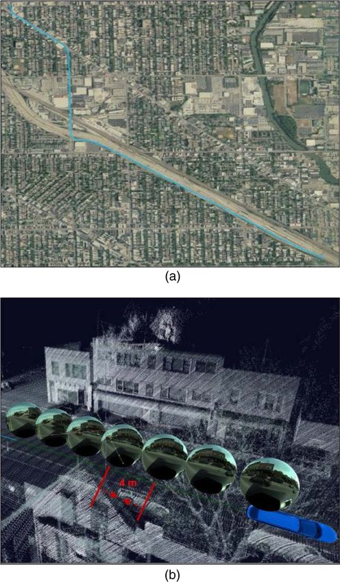
Optical Engineering 54(1), 013108 (January 2015)

                Automatic registration method for mobile LiDAR data
                Ruisheng Wanga,* and Frank P. Ferrieb
                a
                University of Calgary, Department of Geomatics Engineering, Calgary, Alberta T2N 1N4, Canada
                b
                McGill University, Department of Electrical and Computer Engineering and the Center for Intelligent Machines, Montreal,
                Québec H3A 0E9, Canada

                              Abstract. We present an automatic mutual information (MI) registration method for mobile LiDAR and panora-
                              mas collected from a driving vehicle. The suitability of MI for registration of aerial LiDAR and aerial oblique
                              images has been demonstrated under an assumption that minimization of joint entropy (JE) is a sufficient
                              approximation of maximization of MI. We show that this assumption is invalid for the ground-level data. The
                              entropy of a LiDAR image cannot be regarded as approximately constant for small perturbations. Instead of
                              minimizing the JE, we directly maximize MI to estimate corrections of camera poses. Our method automatically
                              registers mobile LiDAR with spherical panoramas over an approximate 4-km drive, and is the first example we
                              are aware of that tests MI registration in a large-scale context. © The Authors. Published by SPIE under a Creative Commons
                              Attribution 3.0 Unported License. Distribution or reproduction of this work in whole or in part requires full attribution of the original publication, including its
                              DOI. [DOI: 10.1117/1.OE.54.1.013108]

                              Keywords: mutual information; registration; mobile LiDAR; panoramas.
                              Paper 141015 received Jun. 27, 2014; accepted for publication Dec. 29, 2014; published online Jan. 27, 2015.

                1 Introduction                                                                              algorithm19 to refine camera parameters estimated from a
                Image-to-range registration is a prerequisite for many appli-                               combination of vanishing point computation and GPS/IMU
                cations. The registration result is critical not only for texture-                          readings. In general, the feature point extraction and robust
                mapping three-dimensional (3-D) models of large-scale                                       matching are the key to a successful registration for this type
                scenes, but also for applications such as image-based upsam-                                of approach.
                pling of range data,1–4 image-guided range segmentation,5,6                                     Instead of matching points, structural feature-based
                and 3-D scene modeling.7 The problem of image-to-range                                      methods11–14 match structural features in both 2-D and 3-
                registration involves the alignment of two-dimensional                                      D space to estimate the relative camera pose. Direct match-
                (2-D) images with 2-D projections of 3-D range data, con-                                   ing single line features is error-prone because of the noise in
                sisting of estimating the relative camera pose with respect to                              both LiDAR and image data as well as the robustness of
                the range sensors.                                                                          the detection algorithms. High-level structural features are
                    There has been a considerable amount of research in                                     helpful to increase the robustness of both detection and
                registering images with range data. Existing methods include                                matching. Wang and Neumann14 registered aerial images
                keypoint-based matching,8–10 structural features-based                                      with aerial LiDAR based on matching so-called “3
                matching,11–14 and mutual information-based registration.15                                 Connected Segments” in which each linear feature contains
                The range data include terrestrial or aerial LiDAR, and the                                 three segments connected into a chain. They used a two-
                images include vertical or oblique aerial images and ground-                                level RANSAC algorithm to refine the putative feature
                level images.                                                                               matches, and estimated camera pose using the method
                    Keypoint-based matching8,10 is based on the similarity                                  described in Ref. 20. Liu et al.11–13 extracted so-called “rec-
                between laser intensity images and corresponding camera                                     tangular parallelepiped” features, which are composed
                images. First, each pixel of the laser intensity image is                                   of vertical or horizontal 3-D rectangular parallelepipeds
                encoded with its corresponding 3-D coordinate. Then, fea-                                   in the LiDAR and 2-D rectangles in the images, to estimate
                ture points are extracted by using either SIFT16 or Förstner                                camera translation with a hypothesis-and-test scheme.
                operators17 from both images. A robust matching strategy                                    Camera rotation was estimated based on at least two
                based on RANSAC18 and/or epipolar geometry constraint                                       vanishing points. Since vanishing points are required,
                is employed to determine the correspondence pairs for com-                                  their methods work well for ground-level data but are
                puting the fundamental matrix. Sensor registration is then                                  not efficient to handle aerial data with a weak perspective
                achieved based on a robust camera spatial resection. Ding                                   effect.
                et al.9 registered oblique aerial images with a 3-D model                                       All the above methods are dependent on either the strong
                generated from aerial LiDAR data based on 2-D and 3-D                                       presence of parallel lines to infer vanishing points, or avail-
                corner features in the 2-D images and 3-D LiDAR model.                                      ability of feature pair correspondence, which limits their
                The correspondence between extracted corners was based                                      applicability and robustness. A recent method15 using statis-
                on a Hough transform and generalized M-estimator sample                                     tical metrics, such as mutual information (MI),21 as a simi-
                consensus. The resultant corner matches are used in Lowe’s                                  larity measure for registering oblique aerial images and aerial
                                                                                                            LiDAR does not require any feature extraction process.
                                                                                                            This method searches for the optimal camera pose through
                *Address all correspondence to: Ruisheng Wang, E-mail: ruiswang@ucalgary                    maximizing the MI between camera images and different
                 .ca                                                                                        attributes of LiDAR such as the LiDAR intensity images,

                Optical Engineering                                                               013108-1                                                      January 2015       •   Vol. 54(1)

Downloaded From: https://www.spiedigitallibrary.org/journals/Optical-Engineering on 29 Jun 2022
Terms of Use: https://www.spiedigitallibrary.org/terms-of-use
Wang and Ferrie: Automatic registration method for mobile LiDAR data

                depth maps, or a combination of both. Instead of using fea-                       blocks of 32 lasers each and the entire unit spins and gen-
                tures, the MI method evaluates statistical measures using all                     erates over 1 × 10⁶ pps. The sensor can spin at rates ranging
                the pixels in both images, which avoids the problems of                           from 5 to 20 Hz, and the default is 10 Hz with a 905-nm
                feature extraction and correspondence. Thus, MI registration                      wavelength. The Ladybug 3 covers more than 80% of a
                method holds the potential to be a robust solution.                               full sphere, with six high quality 1600 × 1200 Sony charge-
                    This paper deals with the problem of the registration                         coupled device sensors, and provides up to 12 MP images
                between mobile LiDAR and spherical panoramas. The                                 at 15 fps. All of these sensors are georeferenced through
                data acquisition platform is designed such that mapping                           a GPS and an IMU.
                between the LiDAR and spherical camera system is
                approximately known through mechanical measurements.
                However, because of vibration induced by motion of the                            3 Method
                platform and deformations arising from temperature                                We start with the work of Mastin et al.15 that registers aerial
                changes, significant registration errors can still occur, requir-                 LiDAR with aerial oblique images based on MI. LiDAR
                ing estimation of the true mapping parameters.                                    intensity images that normally look very similar to gray-
                    In this paper, we use a portion of the LiDAR and spheri-                      scale camera images with, of course, a much lower resolu-
                cal panoramas (i.e., one-sixth of the entire panorama) for                        tion. This correlation makes MI a suitable measure to
                MI computation as we project them onto a plane with a                             evaluate their similarity. In Ref. 15, they define pðx; yÞ and
                view port of 940 × 452 pixels through OpenGL rendering.                           lðx; yÞ as the intensity camera image and projected LiDAR
                In contrast to Mastin et al.,15 we explicitly use the MI metric                   features, respectively, on the xy image plane. For a specific
                as the similarity measure. In their work, which involved                          camera matrix T, the projected LiDAR features are given by
                the registration of aerial LiDAR with oblique images, it                          lT . MI-based registration methods find the optimal camera
                was assumed that the entropy of the LiDAR images                                  matrix that maximizes the MI between camera images and
                remained approximately constant for small perturbations.                          projected LiDAR features
                Under this assumption, minimizing the joint entropy (JE)
                is equivalent to maximizing the MI. However, as we                                T MI ¼ arg max Iðp; lT Þ:                                      (1)
                show in Sec. 3, this approach does not appear to work                                        T
                for the case of ground-based applications such as those con-
                sidered in this paper. The statistics of the data are such that                      They use a generic camera model, the finite projective
                the constant entropy assumption breaks down, invalidating                         camera as described in Ref. 20. Under this camera model,
                the use of JE.                                                                    a point in space is mapped to the point on the image
                    The algorithm presented in this paper is fully automatic                      plane by
                and has been designed to run efficiently on a metropolitain
                LiDAR/spherical image database using different representa-
                tions of LiDAR from those in Mastin et al. We are not aware                       P ¼ KR½Ij − C;                                                (2)
                of any other examples of MI registration that have been
                attempted on this scale.                                                          where C ¼ ½Cx ; Cy ; Cz T is the camera center, I is the
                                                                                                  identity matrix, and R is the camera rotation matrix.
                2 Data Acquisition                                                                R ¼ Rx ðγÞRy ðβÞRz ðαÞ is given by the three rotation matri-
                                                                                                  ces, where α, β, and γ are the Euler angles representing
                Data are collected from a mobile mapping system shown
                                                                                                  yaw, pitch, and roll. The matrix K is the camera calibration
                in Fig. 1, which is composed of a 360 deg LiDAR sensor
                                                                                                  matrix.
                (Velodyne HDL-64E), six high-resolution cameras, a
                                                                                                     In this paper, we show that their assumption is invalid for
                Ladybug 3 camera, GPS, inertial measurement unit (IMU),
                                                                                                  the ground-based case, as small perturbations in camera
                and distance measurement instrument. The Velodyne LIDAR
                                                                                                  pose have larger effect on the LiDAR rendering in the
                sensor consists of 64 lasers mounted on the upper and lower
                                                                                                  ground-level data. The entropy of a LiDAR image cannot
                                                                                                  be regarded as approximately constant for small perturba-
                                                                                                  tions. This is demonstrated by a perturbation analysis,
                                                                                                  which shows how the normalized MI and JE vary around
                                                                                                  the initial registration in terms of altered camera poses
                                                                                                  as shown in Fig. 2. We select four representative scenes
                                                                                                  for this test from Fig. 8. Since the correct registration
                                                                                                  value should be near the initial registration, we set all
                                                                                                  parameters at their initial values and vary each parameter
                                                                                                  to view the shape of the cost functions. The range of camera
                                                                                                  parameter perturbations is 2 units, meters for translation
                                                                                                  and degrees for orientation. The step size for the perturba-
                                                                                                  tion analysis is 0.1 units, for a total of 40 measurements for
                                                                                                  each of the charts shown in Fig. 2. As shown in the figures,
                                                                                                  the x-axis corresponds to relative displacement and the y-
                                                                                                  axis corresponds to the normalized value of MI. The traces
                                                                                                  labeled 1, 2, 3, and 4 in Fig. 2(a)–2(l) correspond to images
                                                                                                  1, 4, 5, and 8 in Fig. 8, respectively. The remaining
                           Fig. 1 NAVTEQ TRUE mobile mapping system.                              trace, data5, rendered as a solid black line in each chart,

                Optical Engineering                                                        013108-2                                     January 2015   •   Vol. 54(1)

Downloaded From: https://www.spiedigitallibrary.org/journals/Optical-Engineering on 29 Jun 2022
Terms of Use: https://www.spiedigitallibrary.org/terms-of-use
Wang and Ferrie: Automatic registration method for mobile LiDAR data

                                       Fig. 2 Probe analysis on camera translation and orientation parameters for evaluation of normalized
                                       mutual information (MI) and joint entropy (JE): (a) X displacements MI. (b) X displacements JE.
                                       (c) Roll displacements MI. (d) Roll displacements JE. (e) Y displacements MI. (f) Y displacements
                                       JE. (g) Pitch displacements MI. (h) Pitch displacements JE. (i) Z displacements MI. (j) Z displacements
                                       JE. (k) Yaw displacements MI. (l) Yaw displacements JE.


                corresponds to the mean values of the other traces and                                                 z
                indicates the general trend. Note that in all cases, the nor-                     θ ¼ arccos p ffiffiffiffiffiffiffiffiffiffiffiffiffiffiffiffiffiffiffiffiffiffiffi
                                                                                                                                     ffi  ;      φ ¼ arctan 2ðy; xÞ;        (3)
                                                                                                               x2 þ y2 þ z 2
                malized MI yields an unambiguous maximum, whereas
                the JE measure is ambigous in most cases. Hence, our con-                         where θ is the inclination ðθ ∈ ½0; πÞ, and φ is the azimuth
                clusion is that JE is an inappropriate metric for use in the                      ðφ ∈ ð−π; πÞ. Each point’s corresponding location in the
                case of ground-level data.                                                        panoramic image ðr; cÞ is computed by Eq. (4)


                                                                                                         θ                                  φ
                3.1 Coordinate Framework                                                          r ¼ int H ;              c ¼ int             þ 0.5 W ;                  (4)
                                                                                                         π                                  2π
                Our panoramic images are generated from a Ladybug III sys-
                tem consisting of six Fisheye cameras, and the individual
                images are then stitched together via α blending. The result-                     where H and W are the height and width of the panoramic
                ing mosaic is transformed into a spherical panorama via                           images, respectively.
                a cylindrical equidistant projection as shown in Fig. 3(a).
                To generate a linear perspective image, such as the one cor-                      3.2 Mutual Information Registration
                responding to the spherical panorama in Fig. 3(a) and shown                       MI methods have been widely used for the multimodal
                in Fig. 3(b), the panorama is mapped onto a sphere and                            registration problem in the medical imaging domain (e.g.,
                viewed from the center (virtual camera).                                          registration of CT and MRI). Recently, they also have been
                   Both LiDAR and image data are georeferenced. We first                          applied to the problem of registering airborne LiDAR data
                convert the geographic coordinates (latitude and longitude)                       with oblique aerial images.15 The MI of two random varia-
                into Earth-centered, Earth-fixed (ECEF) coordinates, and                          bles X and Y can be defined as
                then they are transformed into local tangent plane (LTP)
                coordinates. All computations are based on LTP coordi-                                         Z Z
                                                                                                                                      pðx; yÞ
                nates. Each LiDAR point p ¼ ðx; y; zÞT in LTP coordinates                         IðX; YÞ ¼            pðx; yÞ log                 dxdy;                  (5)
                is converted into spherical coordinates ðθ; φÞ by Eq. (3)                                        Y   X              p1 ðxÞp2 ðyÞ

                Optical Engineering                                                        013108-3                                              January 2015   •   Vol. 54(1)

Downloaded From: https://www.spiedigitallibrary.org/journals/Optical-Engineering on 29 Jun 2022
Terms of Use: https://www.spiedigitallibrary.org/terms-of-use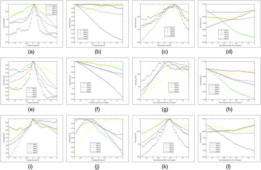
Wang and Ferrie: Automatic registration method for mobile LiDAR data

                                                                                                  new LiDAR images are generated at each iteration during
                                                                                                  the optimization process. Both LiDAR and spherical images
                                                                                                  are rendered onto a plane from the camera center using
                                                                                                  OpenGL for the MI evaluation under a pinhole camera model.
                                                                                                  The perspective camera image is generated by rendering the
                                                                                                  spherical panorama with a view port of 940 × 452 pixels.
                                                                                                  The LiDAR dataset is normally very large. In our experi-
                                                                                                  ments, each scene contains 8 × 10⁶ LiDAR points. To make
                                                                                                  3-D rendering efficient, we also integrate the OpenGL ren-
                                                                                                  dering of the LiDAR features into the registration pipeline to
                                                                                                  speed up the optimization process.
                                                                                                      We use three different representations of the LiDAR data
                                                                                                  with spherical panoramas for evaluating MI. The first repre-
                                                                                                  sentation of LiDAR is the projected LiDAR points with
                                                                                                  intensity information [see Fig. 4(b)]. We call it a LiDAR
                                                                                                  intensity image which looks similar to a gray-scale camera
                                                                                                  image. We use 256 bins for representing LiDAR intensity
                                                                                                  images. The second representation is the projected LiDAR
                                                                                                  points without intensity information [see Fig. 4(c)]. We
                                                                                                  use two bins for representing the binary images. The third
                                                                                                  is the depth map of the LiDAR point cloud [see Fig. 4(d)].
                                                                                                  The point cloud is rendered with depth intensities with
                                                                                                  256 bins, where brighter points indicate a further distance
                                                                                                  to the camera center. We use gray-scale camera images
                                                                                                  instead of color images [see Fig. 4(a)] for the MI compu-
                                                                                                  tation. Note that the bin size in each of the three cases is
                Fig. 3 (a) Spherical panorama generated from six spherical images.                determined by quantization, e.g., 8-bits for intensity and
                (b) Linear perspective view corresponding to the spherical panorama.              1-bit for the binary image corresponding to the LiDAR pro-
                                                                                                  jection in the image plane. The choice of normalization for
                                                                                                  depth on the interval [0, 255] was empirically determined.
                where pðx; yÞ is the joint probability density function of X                      We did not investigate the effect of different quantizations
                and Y, and p1 ðxÞ and p2 ðyÞ are the marginal probability den-                    in this study.
                sity functions of X and Y, respectively. The problem here is                          We use the Nelder-Mead downhill simplex method22 to
                to estimate the correction of the relative camera pose                            optimize the cost function as it does not require derivatives
                between the LiDAR sensor and the Ladybug camera. The                              of the cost function. It is a commonly used nonlinear opti-
                spherical panorama is chosen as a fixed image, because                            mization technique that is well suited to multidimensional,
                the camera view point has to stay in the center of the sphere                     unconstrained minimization as is the case here. As it is appli-
                to generate perspective images. Once the camera moves out                         cable only to convex minimization, we must ensure that
                of the sphere center, the spherical image will be distorted.                      the initial starting point is in the vicinity of the correct local
                The LiDAR image is selected as a moving image, where                              minimum. In practice, we know the approxiate rotation and

                                       Fig. 4 Camera image and three representations of LiDAR point clouds in a same scene: (a) camera gray-
                                       scale image, (b) LiDAR intensity image, (c) LiDAR points, (d) LiDAR depth map.

                Optical Engineering                                                        013108-4                                       January 2015   •   Vol. 54(1)

Downloaded From: https://www.spiedigitallibrary.org/journals/Optical-Engineering on 29 Jun 2022
Terms of Use: https://www.spiedigitallibrary.org/terms-of-use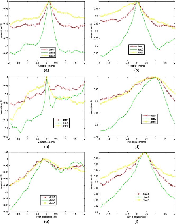
Wang and Ferrie: Automatic registration method for mobile LiDAR data
Fig. 7 Optical image (a) and LIDAR image (b) with 15 manually
selected correspondence points.
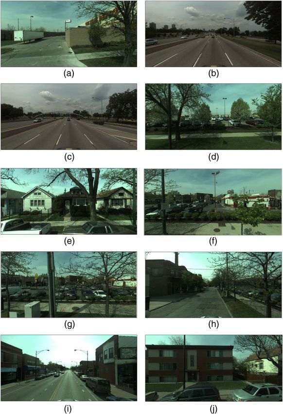
between each sperical panorama is around 4 m. The test data
were collected in the northwestern suburban of Chicago,
Illinois, which include residential, urban streets, and high-
way scenes. The data are in binary format containing around
4 GB LiDAR data (about 226 × 106 points) and 1 GB pano-
ramic images (814 spherical panoramas). We use the camera
views perpendicular to or parallel to the vehicle driving
direction to generate perspective images. Figure 6 illustrates
the camera views vertical to the vehicle driving direction.
Fig. 5 Test data: (a) test data overview, (b) an illustration of the data.
The distance between each camera (e.g., C1 , C2 ) is around
4 m as the images are taken around every 4 m. The camera
translation parameters by virtue of measurements of the data views parallel to the driving direction are similar to Fig. 6
acquisition platform, making finding a suitable starting point except the camera view points to the front.
straightforward. For our analysis, we selected 10 representative urban
scenes shown in Fig. 8 for the evaluation using the three dif-
ferent representations of the LiDAR data described earlier.
4 Experiments Images 1 and 2 show a parking lot in a commercial area (pos-
For the experiments, we made the algorithm automatically sibly shopping mall) from differnet viewpoints. Images 3 and
run through an approximate 4-km drive. The driving routine 4 show a urban street in two different scenarios: with or
is shown with the light blue line in Fig. 5(a). An illustration without trees. Images 5 and 6 show two different residential
of the collected data is shown in Fig. 5(b), where the distance areas. Images 6 and 7 show two different highway scenes.
Image 9 shows a scene where trees are major objects, and
image 10 shows a scene where houses are major objects.
We start with an approximate initial registration that is deter-
mined from the data acquisition platform. The initial camera
pose corrections are set to zero. The optimization will com-
pute the final camera corrections. The experiments were per-
formed on a laptop PC with a dual core 2.60 GHz processor
and 2 GB of RAM. The NVIDIA Quadro NVS 135 M video
card was used. The registration algorithms were imple-
mented in C++, and the implementations of MI and amoeba
optimization were from insight segmentation and registration
toolkit.23 We adjust the tolerances on the optimizer to define
Fig. 6 Camera configuration. convergence. The tolerance on the six parameters is 0.1 (the
Optical Engineering 013108-5 January 2015 • Vol. 54(1)
Downloaded From: https://www.spiedigitallibrary.org/journals/Optical-Engineering on 29 Jun 2022
Terms of Use: https://www.spiedigitallibrary.org/terms-of-use
Wang and Ferrie: Automatic registration method for mobile LiDAR data

                                       Fig. 8 Images used for experiments: (a) Image 1; (b) Image 2; (c) Image 3; (d) Image 4; (e) Image 5;
                                       (f) Image 6; (g) Image 7; (h) Image 8; (i) Image 9; (j) Image 10.

                unit for translation parameters is meters and degrees for ori-                    histograms in terms of the offset errors (pixels) among
                entation parameters). We also set the tolerance on the cost                       these correspondence points) for the scene indicated
                function value to define convergence. The metric returns the                      by Fig. 8(a) (Image 1) before registration, and Image 1A
                value of MI, for which we set the tolerance to be 0.001 bits.                     shows the corresponding pixel offsets after registration.
                The initial size of the simplex is set to 1, and the maximum                      The horizontal axis corresponds to the pixel offsets,
                iteration number is set to 200. In our experiments, almost                        and the vertical axis corresponds to the frequency. Image
                all registrations converged in less than 150 iterations.                          1B shows that most of the pixel offsets are 2 pixels, and
                                                                                                  Image 1A shows that most of the pixel offsets are within
                4.1 Performance Evaluation                                                        1 pixel after MI registration. A similar interpretation applies
                To quantitatively measure the registration results, we com-                       to the rest of the figures. Figure 10 shows the computed
                pare the registration accuracy in terms of pixel offset                           Euclidean distance histograms of the correspondence
                between LiDAR and camera images before and after the                              points for all the 10 images before and after registration.
                registration. We manually selected 15 correspondence                              Before the MI registration, most correspondence points
                points in each spherical image and LiDAR intensity                                have 2 to 3 pixel errors. After the registration, most of
                image. Figure 7 shows an example of a spherical image                             the correspondence points are within 1 pixel. The pixel
                and a LIDAR intensity image marked with 15 correspon-                             offset histograms using other LiDAR representations are
                dence points. Figure 9 shows the computed Euclidean                               similar.
                distance histogram of the correspondence points for                                  Table 1 shows the run time for the 10 representative
                each scene in Fig. 8. In Fig. 9, for instance, Image 1B                           scenes. Testing on the 4-km drive shows that using the
                shows the histogram of the pixel offsets (we compute the                          LiDAR points without intensity normally runs quickly

                Optical Engineering                                                        013108-6                                     January 2015   •   Vol. 54(1)

Downloaded From: https://www.spiedigitallibrary.org/journals/Optical-Engineering on 29 Jun 2022
Terms of Use: https://www.spiedigitallibrary.org/terms-of-use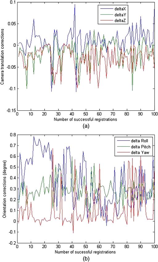
Wang and Ferrie: Automatic registration method for mobile LiDAR data

                                       Fig. 9 Registration error analysis, X -axis stands for pixels, and Y -axis stands for the frequency:
                                       (a) Image 1B; (b) Image 1A; (c) Image 2B; (d) Image 2A; (e) Image 3B; (f) Image 3A; (g) Image 4B;
                                       (h) Image 4A; (i) Image 5B; (j) Image 5A; (k) Image 6B; (l) Image 6A; (m) Image 7B; (n) Image 7A;
                                       (o) Image 8B; (p) Image 8A; (q) Image 9B; (r) Image 9A; (s) Image 10B; (t) Image 10A.

                with fewer iterations. Using LiDAR points with intensity                          the optimizer searched the parameter space using these three
                normally performs the most robustly followed by using                             different representations of the LIDAR data. The measure
                LiDAR points without intensity and using the LiDAR                                initially increases overall with the number of iterations.
                depth maps. We also study the convergence of the optimiza-                        After about 50 iterations, the metric value reaches a steady
                tion using three different measures of MI. Without loss of                        state without further noticeable convergence.
                generality, we choose the data shown in Fig. 4 as an example.                         An example of the registration is shown in Fig. 12. After
                Figure 11 shows the sequence of metric values computed as                         MI registration, the misalignment is not noticeable.

                Optical Engineering                                                        013108-7                                    January 2015   •   Vol. 54(1)

Downloaded From: https://www.spiedigitallibrary.org/journals/Optical-Engineering on 29 Jun 2022
Terms of Use: https://www.spiedigitallibrary.org/terms-of-use
Wang and Ferrie: Automatic registration method for mobile LiDAR data

                Table 1 Registration times in minutes for correctly registered images.

                                                         LiDAR without       LiDAR depth
                MI measure        LiDAR intensity           intensity            map

                Image 1                  0.86                 0.51                0.93

                Image 2                  0.93                 0.50                1.08

                Image 3                  1.05                 0.63                0.97

                Image 4                  0.87                 0.55                0.88

                Image 5                  0.70                  0.4                1.06

                Image 6                  0.83                 0.38                0.85

                Image 7                  0.85                 0.38                0.65

                Image 8                  0.73                 0.38                0.87

                Image 9                  0.97                 0.50                0.71

                Image 10                 1.03                 0.50                0.75

                Mean                     0.88                 0.47                0.87

                4.2 Perturbation Analysis
                We plot the normalized MI of Fig. 4(a) in Fig. (13) using the
                three LiDAR attributes. Figure 13 (red intensity, green point
                only, and yellow depth map) demonstrates that each curve
                has a single peak over a subset of the displacement param-
                eters around the initial registration, which demonstrates
                the effectiveness of the maximization of MI for computing
                optimal camera corrections.
                    We also investigated the failure cases. In our experiments,
                the algorithm works well in feature-rich environments such
                as residential areas, but often fails in scenes with sparse fea-
                tures or containing moving objects like cars, particularly                        Fig. 10 Histogram of Euclidean distance of pixel offset for before
                highway scenes. In our case, the highway scenes mostly                            registration (a) and after registration (b). The histograms were gener-
                fail. The partial overlap between LiDAR point clouds and                          ated with samples for all 10 test images.
                camera images is another reason. The LiDAR scanner
                only can reach up to 120 m, while the camera can always
                have a larger field of view than the LiDAR scanner.
                Figures 14(a) and 14(b) show one typical failure case in
                a highway scene. The cars in the camera image [Fig. 14(a)]
                do not appear in the LiDAR image [Fig. 14(b)]. The LiDAR
                image only partially covers the camera image; for instance,
                the trees and buildings in the far distance in the camera
                image do not appear in the LiDAR image. In Ref. 15,
                the authors claim that they only use the image pixels
                with corresponding projected LiDAR points for MI calcu-
                lation and others are considered background points and
                discarded. We tried to discard the background points and
                only use overlapping regions for MI computation, but
                the results were worse than using entire images. When
                using entire images, the background such as sky appears
                similar in both LiDAR and camera images, which largely
                contributes to the MI score. When using overlapping regions
                for MI computation, the LiDAR images contain no sky.
                Therefore, the background is not used in the MI computa-
                tion, which affects the MI evaluation. Failure cases are                          Fig. 11 Mutual information values produced during the registration
                also due to overexposed images [Figs. 14(c) and 14(d)],                           process.

                Optical Engineering                                                        013108-8                                          January 2015    •   Vol. 54(1)

Downloaded From: https://www.spiedigitallibrary.org/journals/Optical-Engineering on 29 Jun 2022
Terms of Use: https://www.spiedigitallibrary.org/terms-of-use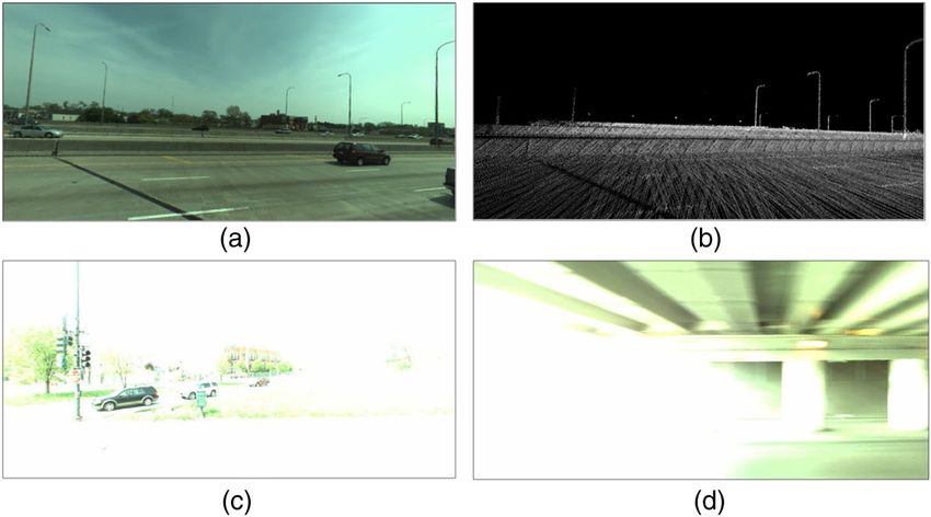
Wang and Ferrie: Automatic registration method for mobile LiDAR data

                                                                                                  particularly in the case where the vehicle drives through/out
                                                                                                  of a tunnel.

                                                                                                  4.3 Camera Pose Corrections
                                                                                                  One of our interests is to investigate how camera pose errors
                                                                                                  change during the data collection. To do so, we manually
                                                                                                  selected 100 successful registrations (using the registrations
                                                                                                  from camera views vertical to the vehicle driving direction)
                                                                                                  by carefully examining the alignment of major features in
                                                                                                  the registered images, and plotting the camera pose correc-
                                                                                                  tions as shown in Fig. 15. Figure 15(a) shows the camera
                            Fig. 12 An example of the registration results.                       translation corrections, and Fig. 15(b) shows the camera

                                       Fig. 13 Plots of normalized mutual information: (a) X displacements. (b) Y displacements. (c) Z dis-
                                       placements. (d) Roll displacements. (e) Pitch displacements. (f) Yaw displacements.

                Optical Engineering                                                        013108-9                                     January 2015   •   Vol. 54(1)

Downloaded From: https://www.spiedigitallibrary.org/journals/Optical-Engineering on 29 Jun 2022
Terms of Use: https://www.spiedigitallibrary.org/terms-of-use
Wang and Ferrie: Automatic registration method for mobile LiDAR data
Fig. 14 Failure cases: (a) Ladybug image. (b) LiDAR image. (c) Overexposed Ladybug image I.
(d) Overexposed Ladybug image II.
orientation corrections. Our observation is that almost all of
the camera translation corrections are within 0.1 m, while the
orientation corrections are within 1 deg.
5 Conclusions and Future Work
In this paper, we have investigated MI registration for
ground-level LiDAR and images. The existing method15
for registering airborne LiDAR with aerial oblique images
does not work on the LiDAR and images collected from
the mobile mapping system, because the assumption used
in Ref. 15 is violated in the case of mobile LiDAR data.
Instead of the minimization of the JE, we use the maximi-
zation of MI for computing optimal camera corrections.
The algorithms work with unstructured LiDAR data and per-
spective rectified panoramic images generated by rendering a
panorama into an image plane using spheric views. We tested
the algorithm on various urban scenes using three different
representations of LiDAR data with camera images for the
MI calculation. Our mutual registration algorithm automati-
cally runs through large-scale mobile LiDAR and panoramic
images collected over a metropolitan scale. It is the first
example we are aware of that tests MI registration in a
large-scale context. With the initiative of urban 3-D model-
ing from location-based service providers such as Nokia and
Google, this work is particularly important for combining
ground-level range and visual data for large-scale photoreal-
istic city modeling.
We generated perspective images from spherical images
using the view either perpendicular or parallel to the vehicle
driving direction. Therefore, we just used one-sixth of the
entire spherical image for the MI registration, which does
not efficiently use all the available information contained
in the 360 deg panoramic images. For future work, one pos-
sible approach would be to project the entire LiDAR points
along with spherical images onto six cube faces using a
quadrilateralized spherical cube mapping24 or other linear
projections. Because the sky and the ground do not provide
much useful information, we actually need just four faces for
Fig. 15 Plots of camera pose corrections using 100 successful regis- the MI registration. To speed up the computation, a multire-
trations: (a) camera translation corrections, (b) camera orientation solution approach can be employed by establishing image
corrections. pyramids on both images. This coarse-to-fine strategy can
Optical Engineering 013108-10 January 2015 • Vol. 54(1)
Downloaded From: https://www.spiedigitallibrary.org/journals/Optical-Engineering on 29 Jun 2022
Terms of Use: https://www.spiedigitallibrary.org/terms-of-useWang and Ferrie: Automatic registration method for mobile LiDAR data
improve the performance of the registration algorithm and Conf. on Computer Vision and Pattern Recognition (CVPR’05),
Vol. 02, pp. 137–143, San Diego, California (2005).
also increases robustness by eliminating local optima at 12. L. Liu and I. Stamos, “A systematic approach for 2D-image to 3D-
coarser levels. One of the limitations of the MI metric is range registration in urban environments,” in Proc. Int. Conf. on
Computer Vision, pp. 1–8, IEEE, Rio de Janeiro, Brazil (2007).
that the intensity histograms contain no spatial information. 13. I. Stamos et al., “Integrating automated range registration with multi-
One possible direction is to incorporate spatial context into view geometry for the photorealistic modeling of large-scale scenes,”
the metric to improve the robustness of the similarity Int. J. Comput. Vis. 78, 237–260 (2008).
14. L. Wang and U. Neumann, “A robust approach for automatic registra-
measure. tion of aerial images with untextured aerial LiDAR data,”IEEE
Beyond these incremental approaches, there are limits to Comput. Soc. Conf. on Computer Vision and Pattern Recognition,
what can be achieved on a practical basis. However, since the CVPR 2009, pp. 2623–2630, IEEE, Miami, Florida (2009).
15. A. Mastin, J. Kepner, and J. Fisher, “Automatic registration of LiDAR
task is 3-D data acquisition, data may be discarded and reac- and optical images of urban scenes,” in Proc. IEEE Comput. Soc. Conf.
quired as necessary. Thus, future research will also be aimed on Computer Vision and Pattern Recognition, pp. 2639–2646, Miami,
at automatic detection of the different failure modes so that Florida (2009).
16. D. G. Lowe, “Distinctive image features from scale-invariant key-
reacquisition can be automatically initiated. points,” Int. J. Comput. Vis. 60, 91–110 (2004).
17. W. Förstner and E. Gülch, “A fast operator for detection and precise
References location of distinct points, corners and centres of circular features,” in
Proc. ISPRS Intercommission Workshop Interlaken, pp. 281–305,
1. J. Diebel and S. Thrun, “An application of Markov random fields to Interlaken, Switzerland (1987).
range sensing,” in Proc. Conf. on Neural Information Processing 18. M. A. Fischler and R. C. Bolles, “Random sample consensus: a para-
Systems (NIPS), Advances in Neural Information Processing Systems, digm for model fitting with applications to image analysis and
Vol. 18, Vancouver, British Columbia (2005). automated cartography,” Commun. ACM, 24(6), pp. 381–395 (1981).
2. J. Dolson et al., “Upsampling range data in dynamic environments,” 19. D. G. Lowe, “Three-dimensional object recognition from single two-
IEEE Comput. Soc. Conf. on Computer Vision and Pattern dimensional images,” Artif. Intell. 31, 355–395 (1987).
Recognition, Vol. 0, pp. 1141–1148, San Francisco, California (2010). 20. R. I. Hartley and A. Zisserman, Multiple View Geometry in Computer
3. L. A. Torres-Méndez and G. Dudek, “Reconstruction of 3D models Vision, 2nd ed., Cambridge University Press, New York (2004).
from intensity images and partial depth,” in Proc. 19th National 21. P. Viola and W. M. Wells III, “Alignment by maximization of mutual
Conf. on Artifical Intelligence, AAAI’04, pp. 476–481, Advancement information,” Int. J. Comput. Vis. 24, 137–154 (1997).
of Artificial Intelligence, San Jose, California (2004). 22. J. A. Nelder and R. Mead, “A simplex method for function minimi-
4. Q. Yang et al., “Spatial-depth super resolution for range images,” IEEE zation,” Comp. J. 7, 308–313 (1965).
Comput. Soc. Conf. on Computer Vision and Pattern Recognition, 23. “Insight segmentation and registration toolkit (ITK),” Kitware Inc,
Vol. 0, pp. 1–8, Minneapolis, Minnesota (2007). http://www.itk.org/ (13 June 2013).
5. M. Deveau et al., “Strategy for the extraction of 3D architectural 24. F. P. Chan and E. M. O’Neill, “Feasibility study of a quadrilateralized
objects from laser and image data acquired from the same viewpoint,” spherical cube earth data base,” Computer Sciences Corp., EPRF Tech.
in Proc. Int. Arch. of Photogrammetry, Remote Sensing and Spatial Report 2-75, Prepared for the Environmental Prediction Research
Information Sciences, Vol. 36, S. El-Hakim, F. Remondino, and Facility, Monterey, California (1975).
L. Gonzo, Eds., Mestre-Venice, Italy (2005).
6. S. Barnea and S. Filin, “Segmentation of terrestrial laser scanning Ruisheng Wang joined the Department of Geomatics Engineering at
data by integrating range and image content,” in Proc. XXIth ISPRS
Congress, International Society for Photogrammetry and Remote the University of Calgary as an assistant professor in 2012. Prior to
Sensing, Beijing, China (2008). that, he had worked as an industrial researcher at NOKIA in Chicago
7. P. Dias et al., “Registration and fusion of intensity and range data for since 2008. He holds a PhD degree in electrical and computer
3D modeling of real world scenes,” in Proc. Int. Conf. on 3D Digital engineering from McGill University, an MSc.E. degree in geomatics
Imaging and Modeling, pp. 418–425, IEEE, Quebec City, Canada engineering from the University of New Brunswick, and a BEng
(2003). degree in photogrammetry and remote sensing from Wuhan
8. S. Becker and N. Haala, “Combined feature extraction for facade University, respectively.
reconstruction,” in Proc. ISPRS Workshop on Laser Scanning,
ISPRS, Espoo, Finland (2007).
9. M. Ding, K. Lyngbaek, and A. Zakhor, “Automatic registration of Frank P. Ferrie received his BEng, MEng, and PhD degrees in
aerial imagery with untextured 3D LiDAR models,” in Proc. Computer electrical engineering from McGill University in 1978, 1980, and 1986,
Vision and Pattern Recognition (CVPR), IEEE, Anchorage, Alaska respectively. Currently, he is a professor in the Department of
(2008). Electrical and Computer Engineering at McGill University and codirec-
10. D. G. Aguilera, P. R. Gonzalvez, and J. G. Lahoz, “An automatic tor of the REPARTI research network in distributed environments.
procedure for co-registration of terrestrial laser scanners and digital His research interests include computer vision, primarily in the areas
cameras,” ISPRS J. Photogramm. Remote Sens. 64, 308–316 (2009). of two and three-dimensional shape analysis, active perception,
11. L. Liu and I. Stamos, “Automatic 3D to 2D registration for the photo- dynamic scene analysis, and machine vision.
realistic rendering of urban scenes,” in Proc. 2005 IEEE Comput. Soc.
Optical Engineering 013108-11 January 2015 • Vol. 54(1)
Downloaded From: https://www.spiedigitallibrary.org/journals/Optical-Engineering on 29 Jun 2022
Terms of Use: https://www.spiedigitallibrary.org/terms-of-useYou can also read