Benchmarking Performance and Power of USB Accelerators for Inference with MLPerf
←
→
Page content transcription
If your browser does not render page correctly, please read the page content below
Benchmarking Performance and Power of
    USB Accelerators for Inference with MLPerf?

 Leandro Ariel Libutti1 , Francisco D. Igual2 , Luis Piñuel2 , Laura De Giusti1 ,
                             and Marcelo Naiouf1
                1
                 Instituto de Investigación en Informática LIDI (III-LIDI)
                           Facultad de Informática, UNLP-CIC
                {llibutti,ldgiusti,mnaiouf}@lidi.info.unlp.edu.ar
           2
               Departamento de Arquitectura de Computadores y Automática
                           Universidad Complutense de Madrid
                                {figual,lpinuel}@ucm.es

        Abstract. The popularization of edge computing imposes new chal-
        lenges to computing platforms in terms of performance, power and en-
        ergy efficiency. A correct tradeoff between these metrics will ultimately
        determine the success or failure of new architectures devoted to infer-
        ence in the road towards an approximation of machine learning to sen-
        sors. In this work, we evaluate the ability of new USB-based inference
        accelerators to fulfill the requirements posed by applications in terms of
        inference time and energy consumption. We propose the adaptation of
        the MLPerf benchmark to handle two new devices: Google Coral Edge
        TPU and Intel NCS2. In addition, we present a hardware infrastructure
        that yields detailed power measurements for USB-powered devices. Ex-
        perimental results reveal interesting insights in terms of performance and
        energy efficiency for both architectures, and also provide useful details
        on the tradeoffs in terms of accuracy derived from the specific arithmetic
        capabilities of each platform.

        Keywords: Edge Computing · Domain-Specific Architectures · USB ·
        Benchmarks · Inference · MLPerf · Google Coral · Intel NCS.

1     Introduction
The emergence of Edge Computing as a convenient strategy to perform Ma-
chine Learning tasks (especifically inference) near sensors [24], reducing laten-
cies and improving response times, has renewed the interest in the integration of
low-power DSAs (Domain-Specific Architectures) [19] into resource-constrained
gateways. These DSAs aim at accelerating inference-specific operations at the
exchange of an affordable power budget. Specifically, USB-based DSAs provide
the ideal combination of flexibility, portability and scalability to Edge Com-
puting deployments, with excellent performance-power ratios, and without the
necessity of specific modifications in the gateways’ architectures.
?
    This work is supported by the EU (FEDER) and Spanish MINECO (TIN2015-65277-
    R, RTI2018-093684-B-I00) and by Spanish CM (S2018/TCS-4423).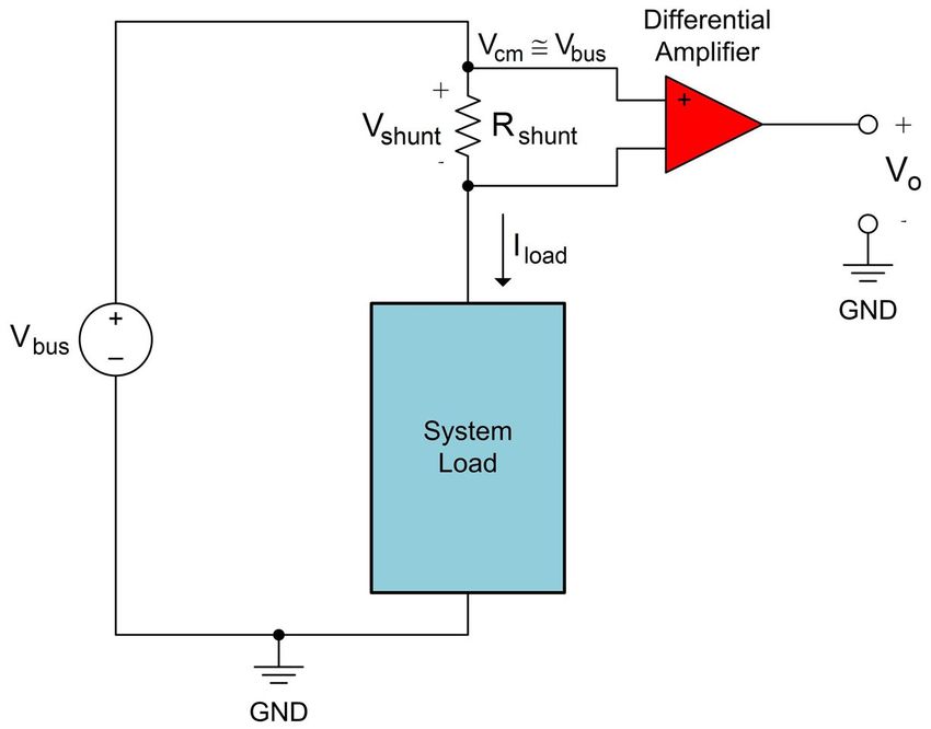
2       L. Libutti et al.

    Among the most popular USB-based machine learning (ML) accelerators are
the Intel Neural Compute Stick 2, featuring an SoC implementation of the Myr-
iad 2 VPU [13] and Google’s Coral USB accelerator, that integrates an Edge
TPU accelerator (adaptation of [21]). Both devices provide an excellent poten-
tial in terms of performance for inference, with power budgets in the terms
of 1 Watt (according to their specifications). In this paper, we investigate on
the actual energy efficiency of both accelerators for common inference work-
loads. Specifically, we provide an empirical study of the performance (in terms
of TOPS/s) and energy efficiency (TOPS/Watt) by adapting the MLPerf infer-
ence benchmark to interact with both devices. In addition, we provide a family
of mechanisms to measure energy consumption for USB devices, and integrate
those measurements within the benchmark. Experimental results reveal clear
performance and energy efficiency gains of the Coral device, at the exchange of
a poorer inference accuracy due to its limitations in floating point support.

2     USB Inference Accelerators
2.1   Google Coral (Google Edge TPU)
The Edge TPU is an ad-hoc ASIC developed by Google, considered a lightweight
version of the TPU provided as part of their cloud services for training neural
networks. The Edge TPU is devoted exclusively to inference, and due to its low
power dissipation it can be found in USB 3.0 versions (the one used in our study)
or integrated into a Coral Devboard SBC (Single Board Computer). The original
TPU implements a 256 × 256 systolic array for matrix-matrix multiplication and
addition; although the detailed specifications of the Edge TPU have not been
disclosed, it is supposed to reduce the dimension of the array to 64×64 for a the-
oretical peak performance of 4 TOPS using 8-bit integers. Hence, models need
to be quantized prior to inferencing, and dequantized as a post-processing stage.
The Google Coral accelerator supports two different modes of operation: starn-
dard frequency, and maximum frequency; the latter promises up to 2× inference
performance, at the exchange of a higher energy consumption and (according to
the documentation) important implications in operating temperature. Section 5
provides a comparative study of both modes.

2.2   Intel NCS2 (Myriad 2 VPU)
The Intel Neural Compute Stick 2 platform implements a System-on-Chip (SoC)
version of the Myriad 2 VPU (Visual Processing Unit). The VPU is a co-
processor aimed at accelerating tensor computation. The Myriad 2 exhibits
12 vector processors (named SHAVE: Streaming Hybrid Architecture Vector
Engines), each one with a large vector register set (32 128-bit registers). The
main functional units include a 128-bit VAU (Vector Arithmetic Unit), CMU
(Compare-and-Move Unit), and 32-bit SAU (Scalar Arithmetic Unit) and IAU
(Integer Arithmetic Unit). Running at 600 Mhz, the maximum declared perfor-
mance is 1 TOPS at the exchange of 1 Watt, with support for 8, 16, 32 and
Benchmarking Performance and Power of USB Accelerators for Inference        3

64-bit integer operations, and FP16/FP32 floating-point operations. In terms of
memory, our setup includes 4 Gbytes of LPDDR3; the memory fabric is designed
for low-latency accesses.
    The NCS2 is distributed as a USB 3.0 device, with a dual-core RISC processor
orchestrating host-to-device communication and managing VPU execution at
runtime. Programming is carried out by means of the NCAPI component (Neural
Compute API), allowing exclusively inference tasks.

3     Software infrastructure. The MLPerf benchmark

The existence of reliable, useful and representative benchmarks is vital in many
fields of computing. In general, and independently from the specific field of appli-
cation, benchmarks should gather basic characteristics in order to succeed [14],
namely: (a) comparability: benchmark scores should characterize software or
hardware systems in such a way that they can be compared and conclusions
about their relative performance be clear and understandable; (b) repeatability:
scores should be kept constant across repetitons of the benchmark under equiv-
alent conditions; (c) well-defined experimentation methodologies: documentation
should cover all details of the underlying mechanisms used to evaluate the sys-
tem, and about the frontend and conditions in which it should be executed; and
(d) configurability: benchmarks should provide tunable knobs to adapt their spe-
cific characteristics to the exact problem to be evaluated. In addition, common
benchmarks usually define a set of specifications, including scenarios, evaluation
criteria, metrics of interest and, obviously, a final score.
     Well-known benchmarks include general-purpose suites, reporting general
scores that gather overall characteristics of the underlying platform; popular
benchmarks include Dhrystone [25], a generic synthetic benchmark that eval-
uates integer computing capabilities, or Whetstone [16], that mainly reports
scores for floating-point arithmetic. The SPEC suite [15] aims at providing in-
dividual benchmarks to measure CPU/GPU capabilities of compute-intensive
codes (SPEC CPU), to evaluate typical paradigms in High Performance Comput-
ing (including MPI, OpenMP, OpenCL, ...) or even Cloud deployments (SPEC
Cloud), to name just a few. Other benchmarks include specific-purpose applica-
tions whose performance is proportional to the floating-point arithmetic capa-
bililities of supercomputers (e.g. LINPACK [17] or HPCG [18]), that are the base
of popular rankings such as Top500 (in terms of peak performance) or Green500
(for energy efficiency).

3.1    MLPerf. Description and internal structure

The aforementioned benchmarks, despite using synthetic tests or real-world ap-
plications, aim at reporting general capabilities of the underlying architectures.
However, in many fields, the importance of reporting performance (or energy-
efficiency) of a given architecture when running a specific type of application
is of key importance. A clear example are training and inference processes on
4 L. Libutti et al.
neural networks in modern general-purpose or domain-specific architectures. A
number of efforts in the field aim at providing de-facto benchmarks that evaluate
the potential of the underlying DSAs or general-purpose architectures. MLPerf
is one of such efforts focusing on ML evaluation.
MLPerf is a specific-purpose benchmark that aims at providing performance
metrics of computing architectures developing training or inference tasks. This
section describes the internal structure of the inference part of MLPerf [23], as is
implemented in version 0.5 of the framework. Figure 1 depicts the basic building
bloks of the framework, interconnections and order in which data flows across
them.
Fig. 1: Data flow in MLPerf Benchmark. Source: [23].
The MLPerf inference benchmark is composed of a number of interconnected
components, namely:
– Input modules, that include the pre-trained model and dataset to be pro-
cessed, and a pre-processor that transforms the raw input data (i.e. images,
strings, . . . ) to a numerical representation that can be processed through
the pipeline.
– Backend and post-processing engine, that ultimately adapt the generic in-
ference query to the specifics of the underlying framework and architecture
that will process it, and post-processes them to check the attained accuracy.
– LoadGen, that generates workloads –queries– and gets performance data
from the inference system.
Within MLPerf, the loads generated by LoadGen implement different sce-
narios, that can be summarized as:Benchmarking Performance and Power of USB Accelerators for Inference 5
– Single Stream, in which the generator sends a query and only upon comple-
tion, the next query is sent.
– Multi Stream, in which the generator sends a set of inferences per query
periodically. This period can be defined between 50 and 100 ms.
– Server, where the system tries to answer each query under a strict pre-
established latency limit.
– Offline, where the complete input dataset is sent in a unique query.
In this work, we leverage the MultiStream mode in order to evaluate a vari-
able batch size and its impact on performance and energy efficiency in both
architectures.
Area Task Model Dataset
Resnet50-v1.5
Vision Image classification (heavy) 25.6M parameters ImageNet (224 × 224)
7.8 GOPS/Image
MobileNet-v1
Vision Image classification (light) 4.2M parameters ImageNet (224 × 224)
1.138 GOPS/Image
Inception-v1
Vision Image classification (heavy) 6.797M parameters ImageNet (224 × 224)
80.6 GOPS/Image
SSD-Resnet34
Vision Object detection (heavy) 36.3M parameters COCO (300 × 300)
433 GOPS/Image
SSD-MobileNet-v1
Vision Object detection (light) 6.91M parameters COCO (300 × 300)
2.47 GOPS/Image
GNMT
Language Machine Translation 210M parameters WMT16 EN-DE
Table 1: Detailed inference benchmarks in MLPerf (source [23]). In bold, models
evaluated in this work.
3.2 Adaptations to use USB accelerators
As said, the execution of the ML model requires a backend matching the specific
software framework used to carry on the inference. MLPerf is equipped with
backends for Tensorflow [10], Tensorflow Lite [8], Pytorch [22] and ONNX [12].
These backends allow performing inferences on CPU and GPU architectures,
but they do not consider specific-purpose architectures such as Google Coral or
the Intel NCS2. To tackle this issue, we have implemented two new backends,
each one matching a different DSA.6 L. Libutti et al.
Tensorflow Lite backend for Google Coral. This backend uses the Tensor-
flow Lite framework, but with slight modifications in the model and inference
prediction process. Executing a model in the Edge TPU requires a prior transla-
tion (re-compilation) of the TFLite model by means of the Edge TPU Compiler,
that maps each TFLite operator to an available operator in the device; if the
original operator is not compatible with the TPU, it is mapped to the CPU.
Hence, by default, a direct execution of a model compiled with TFLite on the
TPU is not possible. The modification of the backend leverages the TFLite del-
egate infrastructure to map the complete graph (or part of it) to the TPU by
means of the corresponding underlying executor specifically distributed by the
manufacturer.
OpenVINO backend for Intel NCS2. The developed backend for the Intel
NCS2 uses the OpenVINO infrastructure [7], that delegates specific tasks to
the underlying NCAPI engine prior to execution. The model received by the
engine is optimized by means of the Intel Model Optimizer [5], that generate a
Intermediate Representation (IR) of the model composed by two files:
– .xml, that describes the network topology.
– .bin, that contains the weights and biases in binary data format.
The neural network represented in these files has 16-bit floating point operations.
3.3 Supported models. Limitations for Coral and NCS2
In order to map a model to the Google Coral USB accelerator, a quantization/d-
equantization process is mandatory. As not all models support this feature, we
have restricted our study of the MLPerf-compliant models to MobileNetV1, and
added InceptionV1 as an additional model, see Table 1. These models have been
evaluated in both archtitectures in order to provide enough comparative perfor-
mance and energy efficiency results.
4 A power measurement infrastructure for USB
accelerators
Our setup is based on a modified USB 3.0 cable in which the power line is
intercepted by means of a shunt resistor to measure the current draw, see Fig-
ure 2 (a); the measurement is performed by a specific IC (Texas Instruments
INA 219) in High Side setup. The INA 219 [4] is an integrated circuit by Texas
Instruments for power measurement that provides digital current/voltage out-
put measurements via I2C/SMBus. In our case, the INA219 is integrated in an
Adafruit board and equipped with a shunt resistor of 0.1Ω, see Figure 2 (b).
There exist a plethora of interaction mechanisms with the INA219 via I2C.
Some of them require external hardware that provide I2C connectivity (e.g.
using an external Raspberry Pi or microcontroller, such as an Adafruit FeatherBenchmarking Performance and Power of USB Accelerators for Inference 7
(b) Adafruit INA219
board.
(c) Digispark I2C-Tiny-
(a) General USB 3.0 cable layout. USB device.
Fig. 2: Diagram of the transformed USB cable to measure consumption through
the USB output, board breakout of the Adafruit INA219 board employed in our
setup and I2C-Tiny-USB device.
HUZZAH featuring an ESP8266 chip), others are simpler and just require a USB-
I2C cable for communication with the host. Among the latter, Bus Pirate [1], or
an USB-MPSSE (Multi-Protocol Synchronous serial Engine) cable [9] provide
the necessary connectivity, see Figure 2 (c).
Entry Value
in0 input Shunt voltage (mV) channel
in1 input Bus voltage (mV) channel
curr1 input Current (mA) measurement channel
power1 input Power (uW) measurement channel
shunt resistor Shunt resistor (uOhm) channel
Table 2: Sysfs entries exposed by I2C-Tiny-USB.
The reported results in Section 5 were extracted by using the I2C-Tiny-USB
firmware [3], an open source hardware/software project by Till Harbaum that
exposes a generic I2C interface attached to the USB bus. Even though the first
versions of the firmware were accompanied by an ad-hoc USB device (based on
an Atmel AVR ATtiny45 CPU), we have leveraged the port to the Digispark
USB Development Board [2], based on the ATtiny85 microcontroller). After8 L. Libutti et al.
a proper configuration, including the load of the corresponding kernel driver,
it is attached to the USB device and make the I2C bus available. No specific
clients are necessary to interact with it, so generic I2C tools, or HWMON [6]
can be used to measure current and/or voltage. Actually, this setup can measure
instantaneous power on virtually any USB device or USB-powered board. Table 2
lists the exposed entries via sysfs used to calculate instantaneous power by
means of the following pseudocode:
f l o a t s h u n t v o l t a g e = i n a 2 1 9 . getShuntVoltage mV ( ) ;
f l o a t b u s v o l t a g e = i n a 2 1 9 . getBusVoltage mV ( ) ;
f l o a t current mA = i n a 2 1 9 . getCurrent mA ( ) ;
f l o a t l o a d v o l t a g e = busvoltage + ( shuntvoltage / 1000) ;
f l o a t power mW = current mA ∗ l o a d v o l t a g e ;
Given the observed inference times (that will be reported in Section 5),
our measurement setup proceeds by using the averaging functionality of the
INA2019. Under these conditions, each read will provide an average value of a
number of samples. This mechanism has been observed to be the optimal trade-
off in terms of precision, overhead and sampling frequency. In our case, we have
configured the INA219 to obtain 32 measures each 17.02ms, gathering average
values for shunt and bus voltage. Hence, the effective sampling frequency is 1.8
KHz, enough for our purposes.
5 Experimental results
5.1 Experimental setup
All experiments have been carried out on an Intel Xeon E3-1225 server running at
3.2 GHz, equipped with 32 Gb of DDR3 RAM. Both hardware accelerators were
attached to the system through an USB 3.0 interface. The software infrastructure
for both architectures includes an Ubuntu 18.04.3 distribution (Linux kernel
version 4.15.0), Tensorflow 2.0, TFLite 1.14 and OpenVINO 2019-R3.1.
In the following, we provide comparative results between both architectures
in terms of performance (inference time), energy efficiency, power consumption,
accuracy tradeoff and MLPerf overhead. All results have been extracted after 8
repetitions of the benchmark and average values are reported. This amount of
repetitions is performed to obtain stable values. When increasing the batch size,
the upper limits in size is extracted by erroneous executions of the benchmark.
5.2 Performance and inference time
Figure 3 provides an overview of the performance (in terms of time per image) for
each model on the two tested architectures. Note that the Google Coral numbersBenchmarking Performance and Power of USB Accelerators for Inference 9
include performnance for standard frequency and for maximum frequency. The
maximum batch size for Intel NCS is 128 because the board does not allow larger
sizes. In terms of inference time, observe that both models and architectures
differ in the exhibited behaviors:
– In the case of MobileNetV1, a direct performance comparison between both
architectures reveals improvements between 3.2×-3.7× for individual infer-
ences (compared with standard-maximum frequency in the Coral) and be-
tween 4.5×-7× for the largest batch size.
– In the case of InceptionV1, the improvements range from 1.5×-1.9× for the
standard frequency, to 3×-4.6× for the maximum frequency. Note, also, that
the attained performance in this case is highly sensible to the batch size.
Therefore, you get better performance by inference on Google Coral.
Performance vs. Batch Size - MobileNetV1 Performance vs. Batch Size - InceptionV1
Coral (standard frequency) Coral (fast frequency) NCS2 Coral (standard frequency) Coral (fast frequency) NCS2
25 25
20 20
Time/image (ms)
Time/image (ms)
15 15
10 10
5 5
0 0
1 10 100 1000 1 10 100 1000
Batch Size (images) Batch Size (Images)
Fig. 3: Comparative performance analysis for Mobilenet V1 (left) and Inception
V1 (right).
5.3 Energy efficiency
Figure 4 reports the energy efficiency of both boards when performing inference
on the described models and dataset, for an increasing batch size. Results are re-
ported in terms of TOPS/Watt up to the maximum batch size supported by each
architecture on MobilenetV1 and InceptionV1. As for the performance results,
energy efficiency is reported on the Google Coral accelerator for standard and
maximum frequency. A key observation is extracted from a direct comparison
between the three setups: in all cases, the Google Coral device exhibits higher
numbers for efficiency. Diving into details, the improvement in terms of efficiency
when comparing Google Coral with the Intel NCS2 is roughly 6.1× when using
the standard frequency, and up to 7.6× for the maximum frequency version for10 L. Libutti et al.
the MobileNetV1 model. For the InceptionV1 model, MLPerf reports a smaller
gap between both architectures, ranging from 4× (standard frequency) and 4.9×
(maximum frequency).
In all cases, note how energy efficiency is much sensible to the batch size in
the case of the Google Coral than for the Intel NCS2. In the latter, efficiency
remains mainly constant independently from the selected batch size for inference.
Energy efficiency vs. Batch size - MobileNet Energy efficiency vs. Batch size - Inception
Coral (standard frequency) Coral (fast frequency) NCS2 Coral (standard frequency) Coral (fast frequency) NCS2
0.1 0.2
0.075 0.15
TOPS/Watt
TOPS/Watt
0.05 0.1
0.025 0.05
0 0
1 10 100 1000 1 10 100 1000
Batch Size (Images) Batch Size (Images)
Fig. 4: Comparative energy efficiency analysis for Mobilenet V1 (left) and Incep-
tion V1 (right).
5.4 Power consumption
Absolute power dissipation is also of great interest due to the tight limitations of
common edge devices in terms of power supply. Figure 5 provides detailed data
of the absolute power draw of both accelerators in terms of peak power consump-
tion, average power performing inference on the MobileNetV1 model, and idle
power consumption. For the Edge TPU, both standard and maximum frequency
is reported. In all cases, results are reported in terms of Watts for an increasing
batch size using the measurement environment described in Section 4. Idle power
is clearly different on the Coral device (around 1 Watt) and on the Intel NCS2
(around 1.5 Watt), which reveals more efficient power saving techinques in the
former. Both average and peak power dissipation (both attained at the infer-
ence engine invocation of MLPerf) reveal similar consumption for the NCS2 and
the Google Coral board running at maximum frequency (around 2 Watts). The
latter running at standard frequency reduces peak power dissipation to values
around 1.6 Watts. It is worth noting that application power heavily depends on
the batch size in the case of the Google Coral, with substantial reductions for
small batch sizes; on the contrary, the Intel NCS2 accelerator maintains constant
both the peak and the average power consumption independently of the batchBenchmarking Performance and Power of USB Accelerators for Inference 11
Coral Power - MobileNetV1 - Std. Frequency Coral Power - MobileNetV1 - Max. Freq.
Peak Power [W] Inference Power [W] Idle Power [W] Peak Power [W] Inference Power [W] Idle Power [W]
2.5 2.5
2 2
1.5 1.5
Power (W)
Power (W)
1 1
0.5 0.5
0 0
1
2
4
8
1
2
4
8
16
32
64
16
32
64
8
6
2
8
6
2
24
48
24
48
12
25
51
12
25
51
10
20
10
20
Batch size (images) Batch size (images)
Intel NCS Power - MobileNet V1
Peak Power [W] Inference Power [W] Idle Power [W]
2.5
2
1.5
Power (W)
1
0.5
0
1
2
4
8
16
32
64
8
12
Batch size (images)
Fig. 5: Comparative power dissipation analysis for Mobilenet.
size. Again, this reveals a higher sophistication in the energy saving mechanisms
in the case of the Google Coral device.
5.5 Accuracy tradeoffs
The aforementioned results reveal clear advantages of the Google Coral board
compared with Intel NCS2 both in terms of performance and energy efficiency.
These advantages, however, come at the exchange of a lower accuracy in the
inference process. Figure 6 provides an overview of such a tradeoff. including
the relation between accuracy and performance (in terms of TOPS) for both
models, and a similar tradeoff comparison in terms of energy efficiency (TOP-
S/W). Points with the same color denote accuracy extracted after inference on
different subsets of the input dataset using batch size equal to 1. Observe how
the greater performance and energy efficiency of the Coral accelerator versus
the Intel NCS2 are in exchange of a lower accuracy for both models. Specifi-
cally, for MobilenetV1, the Intel NCS2 attains an average inference accuracy of
73.7% versus 70.6% attained by the Edge TPU; for InceptionV1, the accuracy
decreases from 69% to 65.9% in average. In both cases, the use of quantization
and INT8 in the Edge TPU is the main motivation behind this difference in
terms of accuracy.12 L. Libutti et al.
Accuracy vs. TOPS Accuracy vs. TOPS/W
Coral - MobileNet V1 Coral - Inception V1 Coral - MobileNet V1 Coral - Inception V1
NCS2 - MobileNet V1 NCS2 - Inception V1 NCS2 - MobileNet V1 NCS2 - Inception V1
80 80
75 75
Accuracy (%)
Accuracy
70 70
65 65
60 60
0.05 0.1 0.15 0.2 0.25 0.025 0.05 0.075 0.1 0.125 0.15
Performance (TOPS) Efficiency (TOPS/W)
Fig. 6: Accuracy versus performance (left) and energy efficiency analysis (right).
5.6 MLperf overhead
The last round of experiments aims at evaluating the overhead introduced by
the MLPerf benchmark compared with a pure inference under identical circum-
stances, mainly due to the pre- and post-processing stages. Figure 7 reports the
observed inference time reported by MLPerf (red line), and the actual inference
time (blue line) for both models on the Google Coral (running at maximum
frequency). The yellow line shows the overhead time percentage in both cases.
Observe how, while the overhead is negligible for large batch sizes –between 1%
and 3%–, it should be considered for small batch sizes, as it increases up to
10%–15% in those cases.
MLPerf vs Inference Only - MobileNetV1 MLPerf vs Inference Only - InceptionV1
Time/Image (Inference Only) Time/Image Overhead Time/Image Time/Image (Inference Only) Overhead
10 15 15 10
8 8
MLPerf overhead (% time)
10 10
Overhead (% time)
Time/image (ms)
Time/image (ms)
6 6
4 4
5 5
2 2
0 0 0 0
1
2
4
8
1
2
4
8
16
32
64
16
32
64
8
6
2
8
6
2
24
48
24
48
12
25
51
12
25
51
10
20
10
20
Batch size Batch size
Fig. 7: MLPerf overhead for MobilenetV1 (left) and InceptionV1 (right) for the
Google Coral accelerator.Benchmarking Performance and Power of USB Accelerators for Inference 13
6 Conclusions and future work
In this paper, we have provided a preliminar performance and energy efficieny
comparison between two state-of-the-art USB-based DSAs: the Intel NCS2 and
the Google Coral USB accelerator. While similar in applicability, both present
different capabilities in terms of accuracy and performance, as reveal our ex-
perimental results. We have also presented a mechanism to measure power con-
sumption for USB-based devices and we have leveraged it to extract actual power
consumption numbers for both architectures.
In addition, modification was developed on MLPerf to support the execution
of machine learning models on USB-based DSAs.
This work is developed in the framework of a line of research that aims at in-
tegrating power measurements in machine learning benchmarks and frameworks,
and that includes evaluations at different levels, including:
– USB and multi-USB accelerator setups.
– Single Board Computers, including BeagleBone AI, Nvidia Jetson Nano and
Google Coral Devboard.
– PCIe devices, leveraging PMLib [11] and an ad-hoc power measurement
framework [20]. Our plan is also to extend the framework to PCI2 devices
attached through M.2 slots.
References
1. Bus pirate. http://dangerousprototypes.com/docs/BusP irate/es, accessed :
2019 − 11 − 8
2. Digispark. http://digistump.com/wiki/digispark, accessed: 2019-11-8
3. I2c tiny usb. https://github.com/harbaum/I2C-Tiny-USB, accessed: 2019-11-8
4. Ina219 online datasheet. http://www.ti.com/lit/ds/symlink/ina219.pdf, accessed:
2019-11-8
5. Intel model optimizer. https://docs.openvinotoolkit.org/latest/ docs MO DG
Deep Learning Model Optimizer DevGuide.html, accessed: 2019-11-8
6. Linux driver for ina2xx. http://www.ti.com/tool/INA2XXSW-LINUX, accessed: 2019-
11-8
7. Openvino toolkit. https://software.intel.com/en-us/openvino-toolkit, accessed: 2019-
11-8
8. Tensorflow lite. https://www.tensorflow.org/lite, accessed: 2019-11-8
9. Usb mpsse. https://www.ftdichip.com/Support/Documents/AppNotes/AN 135
MPSSE Basics.pdf, accessed: 2019-11-8
10. Abadi, M., Agarwal, A., Barham, P., Brevdo, E., Chen, Z., Citro, C., Corrado, G.S.,
Davis, A., Dean, J., Devin, M., Ghemawat, S., Goodfellow, I., Harp, A., Irving, G.,
Isard, M., Jia, Y., Jozefowicz, R., Kaiser, L., Kudlur, M., Levenberg, J., Mané, D.,
Monga, R., Moore, S., Murray, D., Olah, C., Schuster, M., Shlens, J., Steiner, B.,
Sutskever, I., Talwar, K., Tucker, P., Vanhoucke, V., Vasudevan, V., Viégas, F., Vinyals,
O., Warden, P., Wattenberg, M., Wicke, M., Yu, Y., Zheng, X.: TensorFlow: Large-
scale machine learning on heterogeneous systems (2015), https://www.tensorflow.org/,
software available from tensorflow.org14 L. Libutti et al.
11. Alonso, P., Badia, R.M., Labarta, J., Barreda, M., Dolz, M.F., Mayo, R., Quintana-
Ortı́, E.S., Reyes, R.: Tools for power-energy modelling and analysis of paral-
lel scientific applications. In: 41st International Conference on Parallel Processing,
ICPP 2012, Pittsburgh, PA, USA, September 10-13, 2012. pp. 420–429 (2012).
https://doi.org/10.1109/ICPP.2012.57, https://doi.org/10.1109/ICPP.2012.57
12. Bai, J., Lu, F., Zhang, K., et al.: Onnx: Open neural network exchange.
https://github.com/onnx/onnx (2019)
13. Barry, B., Brick, C., Connor, F., Donohoe, D., Moloney, D., Richmond, R., O’Riordan,
M., Toma, V.: Always-on vision processing unit for mobile applications. Micro, IEEE
35, 56–66 (03 2015). https://doi.org/10.1109/MM.2015.10
14. Bouckaert, S., Gerwen, J.V.V., Moerman, I.: Benchmarking computers and computer
networks (2011)
15. Bucek, J., Lange, K.D., v. Kistowski, J.: Spec cpu2017: Next-generation
compute benchmark. In: Companion of the 2018 ACM/SPEC Interna-
tional Conference on Performance Engineering. pp. 41–42. ICPE ’18, ACM,
New York, NY, USA (2018). https://doi.org/10.1145/3185768.3185771,
http://doi.acm.org/10.1145/3185768.3185771
16. Curnow, H., Wichmann, B.: A synthetic benchmark. The Computer Journal 19, 43–49
(02 1976). https://doi.org/10.1093/comjnl/19.1.43
17. Dongarra, J.: The linpack benchmark: An explanation. In: Proceedings of the 1st Inter-
national Conference on Supercomputing. pp. 456–474. Springer-Verlag, London, UK,
UK (1988), http://dl.acm.org/citation.cfm?id=647970.742568
18. Dongarra, J., Heroux, M.A., Luszczek, P.: High-performance
conjugate-gradient benchmark. Int. J. High Perform. Comput. Appl.
30(1), 3–10 (Feb 2016). https://doi.org/10.1177/1094342015593158,
https://doi.org/10.1177/1094342015593158
19. Hennessy, J.L., Patterson, D.A.: Computer Architecture, Sixth Edition: A Quantitative
Approach. Morgan Kaufmann Publishers Inc., San Francisco, CA, USA, 6th edn. (2017)
20. Igual, F.D., Jara, L.M., Pérez, J.I.G., Piñuel, L., Prieto-Matı́as, M.: A power mea-
surement environment for pcie accelerators. Computer Science - R&D 30(2), 115–124
(2015). https://doi.org/10.1007/s00450-014-0266-8, https://doi.org/10.1007/s00450-
014-0266-8
21. Jouppi, N.P., Young, C., Patil, N., Patterson, D.A., Agrawal, G., Bajwa, R., Bates,
S., Bhatia, S., Boden, N., Borchers, A., Boyle, R., Cantin, P., Chao, C., Clark, C.,
Coriell, J., Daley, M., Dau, M., Dean, J., Gelb, B., Ghaemmaghami, T.V., Gottipati,
R., Gulland, W., Hagmann, R., Ho, R.C., Hogberg, D., Hu, J., Hundt, R., Hurt, D.,
Ibarz, J., Jaffey, A., Jaworski, A., Kaplan, A., Khaitan, H., Koch, A., Kumar, N., Lacy,
S., Laudon, J., Law, J., Le, D., Leary, C., Liu, Z., Lucke, K., Lundin, A., MacKean,
G., Maggiore, A., Mahony, M., Miller, K., Nagarajan, R., Narayanaswami, R., Ni, R.,
Nix, K., Norrie, T., Omernick, M., Penukonda, N., Phelps, A., Ross, J., Salek, A.,
Samadiani, E., Severn, C., Sizikov, G., Snelham, M., Souter, J., Steinberg, D., Swing,
A., Tan, M., Thorson, G., Tian, B., Toma, H., Tuttle, E., Vasudevan, V., Walter, R.,
Wang, W., Wilcox, E., Yoon, D.H.: In-datacenter performance analysis of a tensor
processing unit. CoRR abs/1704.04760 (2017), http://arxiv.org/abs/1704.04760
22. Paszke, A., Gross, S., Chintala, S., Chanan, G., Yang, E., DeVito, Z., Lin, Z., Des-
maison, A., Antiga, L., Lerer, A.: Automatic differentiation in pytorch. In: NIPS-W
(2017)
23. Reddi, V.J., Cheng, C., Kanter, D., Mattson, P., Schmuelling, G., Wu, C.J., Anderson,
B., Breughe, M., Charlebois, M., Chou, W., Chukka, R., Coleman, C., Davis, S., Deng,
P., Diamos, G., Duke, J., Fick, D., Gardner, J.S., Hubara, I., Idgunji, S., Jablin, T.B.,Benchmarking Performance and Power of USB Accelerators for Inference 15
Jiao, J., John, T.S., Kanwar, P., Lee, D., Liao, J., Lokhmotov, A., Massa, F., Meng, P.,
Micikevicius, P., Osborne, C., Pekhimenko, G., Rajan, A.T.R., Sequeira, D., Sirasao,
A., Sun, F., Tang, H., Thomson, M., Wei, F., Wu, E., Xu, L., Yamada, K., Yu, B.,
Yuan, G., Zhong, A., Zhang, P., Zhou, Y.: Mlperf inference benchmark (2019)
24. Satyanarayanan, M.: The emergence of edge computing. Computer 50(1), 30–39 (Jan
2017). https://doi.org/10.1109/MC.2017.9, https://doi.org/10.1109/MC.2017.9
25. Weicker, R.P.: Dhrystone: A synthetic systems programming benchmark. Com-
mun. ACM 27(10), 1013–1030 (Oct 1984). https://doi.org/10.1145/358274.358283,
http://doi.acm.org/10.1145/358274.358283You can also read