Carbon export and fate beneath a dynamic upwelled filament off the California coast
←
→
Page content transcription
If your browser does not render page correctly, please read the page content below

Biogeosciences, 18, 3053–3086, 2021
https://doi.org/10.5194/bg-18-3053-2021
© Author(s) 2021. This work is distributed under
the Creative Commons Attribution 4.0 License.

Carbon export and fate beneath a dynamic upwelled filament
off the California coast
Hannah L. Bourne1 , James K. B. Bishop1,2 , Elizabeth J. Connors1,3 , and Todd J. Wood2
1 Dept. of Earth and Planetary Science, University of California, Berkeley, CA, 94720, USA
2 Earth and Environmental Sciences Division, Lawrence Berkeley National Laboratory, Berkeley, CA, 94720, USA
3 Scripps Institution of Oceanography, La Jolla, CA, 92093, USA

Correspondence: James K. B. Bishop (jkbishop@berkeley.edu)

Received: 17 September 2020 – Discussion started: 30 September 2020
Revised: 26 March 2021 – Accepted: 6 April 2021 – Published: 20 May 2021

Abstract. To understand the vertical variations in carbon          1   Introduction
fluxes in biologically productive waters, four autonomous
carbon flux explorers (CFEs), ship-lowered CTD-interfaced          Carbon export driven by the biological carbon pump, the pro-
particle-sensitive transmissometer and scattering sensors,         cess by which photosynthetically derived biomass is trans-
and surface-drogued sediment traps were deployed in a fila-        ported out of the surface layer, is an important component
ment of offshore flowing, recently upwelled water, during the      of the global carbon cycle. Atmospheric carbon concentra-
June 2017 California Current Ecosystem – Long Term Eco-            tions are in part controlled by the depth at which sinking or-
logical Research process study. The Lagrangian CFEs op-            ganic matter is remineralized (Kwon et al., 2009) yet the fate
erating at depths from 100–500 m yielded carbon flux and           of carbon exported to deeper waters beneath highly produc-
its partitioning with size from 30 µm–1 cm at three intensive      tive coastal regions is poorly understood. Current estimates
study locations within the filament and in waters outside the      for global carbon export range from 5 to > 12 Pg C yr−1
filament. Size analysis codes intended to enable long-term         (Boyd and Trull, 2007; Henson et al., 2011; Li and Cassar,
CFE operations independent of ships are described. Differ-         2016; Dunne et al., 2005; Siegel et al., 2014, 2016; Yao and
ent particle classes (anchovy pellets, copepod pellets, and        Schlitzer, 2013). Because coastal upwelling regions are such
> 1000 µm aggregates) dominated the 100–150 m fluxes dur-          productive and unique ecosystems with complex current in-
ing successive stages of the filament evolution as it pro-         teractions, a question to be asked is as follows: is export of
gressed offshore. Fluxes were very high at all locations in        material to depth in these systems different than in open-
the filament; below 150 m, flux was invariant or increased         ocean environments?. If so, knowing the rules governing par-
with depth at the two locations closer to the coast. Martin        ticulate carbon export and remineralization in these regions
curve b factors (± denotes 95 % confidence intervals) for to-      will significantly advance carbon cycle simulations of CO2
tal particulate carbon flux were +0.37 ± 0.59, +0.85 ± 0.31,       uptake by the oceans.
−0.24 ± 0.68, and −0.45 ± 0.70 at the three successively oc-          While ocean colour satellites provide the temporal and
cupied locations within the plume, and in transitional waters.     spatial scale of phytoplankton biomass when clouds permit,
Interestingly, the flux profiles for all particles < 400 µm were   flux beneath the euphotic zone is much more difficult to ob-
a much closer fit to the canonical Martin profile (b − 0.86);      serve and therefore not as well known. A number of recent
however, most (typically > 90 %) of the particle flux was car-     studies have noted discrepancies in reconciling meso- and
ried by > 1000 µm sized aggregates which increased with            bathypelagic activity with current euphotic zone flux esti-
depth. Mechanisms to explain the factor of 3 flux increase         mates (Banse, 2013; Burd et al., 2010; Ebersbach et al., 2011;
between 150 and 500 m at the mid-plume location are inves-         Passow and Carlson, 2012; Stanley et al., 2012). Measure-
tigated.                                                           ments of new production (NP; Eppley and Peterson, 1979)
                                                                   should balance particle export measured at the same time
                                                                   if gravitational particle sinking dominates export; however,

Published by Copernicus Publications on behalf of the European Geosciences Union.
3054                                      H. L. Bourne et al.: Carbon export and fate beneath a dynamic upwelled filament

                                                                     files that do not decrease monotonically with depth as pre-
                                                                     dicted by Martin’s formula have been observed, especially
                                                                     in regions that are both physically and biologically dynamic
                                                                     (e.g. Bishop et al., 2016, in the Santa Cruz Basin; Giering et
                                                                     al., 2017, in the North Atlantic), suggesting additional mech-
                                                                     anisms contributing to particle flux are at play.
                                                                        The California Current, the eastern boundary current of
                                                                     the North Pacific gyre, flows south from the sub-arctic North
                                                                     Pacific. Beneath it, the subsurface California Undercurrent
                                                                     flows poleward at depths between 200 and 500 m, with strong
                                                                     seasonal variability (Lynn and Simpson, 1987). Along the
                                                                     coast, the complex interactions of filaments, geostrophic
                                                                     flow, wind-driven Ekman transport, and mesoscale eddies
                                                                     distribute coastal waters. This leads to a heterogeneous pat-
                                                                     tern of productivity in surface waters with some regions (of-
Figure 1. Martin curves normalized to 150 m. Representative data     ten in the vicinity of headlands) having very high productiv-
from Martin et al. (1987), Buesseler et al. (2007), and Bishop et    ity near centres of coastal upwelling, while others have inter-
al. (2016). b values of lines from left to right are −1.33 (Stn.     mediate productivity spurred by wind stress curl upwelling
ALOHA), −0.86 (VERTEX I), −0.51 (Stn. K2), −0.19, and −0.3
                                                                     and other low-productivity regimes which reflect the onshore
(March and January 2016, Santa Cruz Basin). Transport efficiencies
                                                                     flow of oligotrophic waters (Gruber et al., 2011; Ohman et
between 150 and 500 m range from 20 % (ALOHA) to 80 % (Santa
Cruz Basin).                                                         al., 2013; Siegelman-Charbit et al., 2018). In the summer,
                                                                     winds blowing south along the California coast cause surface
                                                                     waters to divert to the west, which allows deep nutrient-rich
NP often is higher than particle export (Bacon et al., 1996;         cold water to come to the surface. This water coming to the
Estapa et al., 2015; Stukel et al., 2015). Mechanistic under-        surface moves offshore in filaments which can extend off-
standing of these differences is thus important to food web          shore several hundred kilometres.
models.                                                                 The California Current Ecosystem Long-Term Ecological
   The strength and efficiency of the biological carbon pump         Research (CCE-LTER) process study (1 June–2 July 2017;
are governed by complex interactions between phytoplank-             P1706) gave us the opportunity to observe carbon flux pro-
ton, zooplankton, and physical mixing. The Martin curve              files beneath a rapidly evolving surface filament over its life-
(Eq. 1), an empirical relationship, was derived from surface-        time and to understand the magnitude, scales, and mech-
tethered sediment trap observations made in the North Pacific        anisms of coastal production and its transport. During the
during the VERTEX programme (Martin et al., 1987),                   study, we deployed carbon flux explorers (CFEs; Bishop
                                                                     et al., 2016, and Bourne et al., 2019) to depths of 500 m
                      b
                                                                     to observe particle flux variability and specifics of particle

                z
F = Fref                   ,                                  (1)    classes contributing to flux. Figure 2 shows the locations of
               zref
                                                                     CFE deployments and other activities during the CCE-LTER
where F is flux at depth z, Fref is the flux measured at a           study, the Santa Cruz Basin (SCB) study site of Bishop et
reference depth zref (usually near the base of the euphotic          al. (2016), and the coastal station VERTEX 1 (Martin et al.,
zone), and b is a constant. Martin et al. (1987) found the best      1987). The CCE-LTER study combined spatial surveys, three
fits with b = −0.86. The choice of zref does not influence the       cross-filament CTD transects, and four sequentially num-
derived b value.                                                     bered multi-day quasi-Lagrangian intensive sampling “cy-
   Bishop (1989) compared the Martin and six other formu-            cles” within and outside of the filament. Cycles 1 to 4 cor-
lations for particle flux at depth in the open ocean and found       respond to locations 1 to 4 which are referred to as L1 to L4
that the Martin curve for predicting flux was most robust;           below. L1, L2, and L4 represent sampling during the early,
while many profiles were fit with the classic Martin b factor        intermediate, and late stages of filament evolution. The order
of −0.86, the study found (in rare cases) b values of −0.3           of occupations of L3 (outside of the filament) and L4 enabled
to −1.5. Subsequent studies in the open ocean have yielded           a more complete view of filament evolution.
similarly varying b values, and all show the expected flux de-          In this study, we report autonomously measured carbon
crease with depth (Fig. 1) (Buesseler et al., 2007; Lutz et al.,     flux profiles in the mesopelagic zone beneath a filament of
2007; Marsay et al., 2015).                                          upwelled water off the coast of California and the finding
   If all material sinking to depth is assumed to be gravita-        at two locations (L1 and L2) that flux was invariant or in-
tionally exported material originating from a stable photo-          creasing with depth, while flux decreased more slowly than
synthetically derived source in the euphotic zone, an increase       predicted by the Martin formula at two other locations. We
in material with depth should not occur. However, flux pro-          explore mechanisms for these flux profile observations. In the

Biogeosciences, 18, 3053–3086, 2021                                                     https://doi.org/10.5194/bg-18-3053-2021
H. L. Bourne et al.: Carbon export and fate beneath a dynamic upwelled filament                                                    3055

Figure 2. (a) CFE and CTD deployments at locations L1 to L4.
The CTD stations were close to a drifting surface-drogued produc-
tivity array. For the majority of stations, the CTDs and CFEs were
close to one another. However, at L2, the CFEs diverged to the west-
northwest of the drogued drifters. Dots depict locations of cross-
filament CTD particle–optics transects T1, T2, and T3. T1 preceded
work at L1; T2 was occupied after completion of sampling at L2.
T3 was completed after work at L4. Data from transects shown in
Fig. 11. (b) CFE-Cal during recovery.

following discussion, we use the term “non-classic” to rep-
resent strong departures from the classic (b = −0.86) Martin
curve.

Study area                                                             Figure 3. Remotely sensed surface chlorophyll (a, c, e, g) and sea
                                                                       surface temperature (SST) (b, d, f, h) maps of the study area from
The June 2017 CCE-LTER process study aboard R/V Revelle                late May to the end of June 2017. All images are from 4 km resolu-
followed a strong filament of upwelled cold, high-salinity             tion, 8 d averaged data from VIIRS on the Suomi NPP satellite. The
                                                                       stars represent locations 1 to 4 where CFEs were deployed. Stars
westward-flowing water off the coast of California. In late
                                                                       are filled in the panels most closely corresponding to the time of
May, cold water upwelled along the coast due to the in-
                                                                       observations.
tensification of upwelling-favourable north to south winds;
shortly thereafter a filament developed near Morro Bay
(35◦ 220 N, 122◦ 520 W, Fig. 2) and began propagating west-
                                                                       Zone Colour Scanner (CZCS) data to provide context for the
ward (Fig. 3a, b). Eventually, the filament extended 250 km
                                                                       June 1984 Martin et al. (1987) VERTEX 1 station. Sea sur-
offshore (Fig. 3c, d). By mid-June, the westernmost filament
                                                                       face height (SSH) data (derived from a suite of spacecraft)
waters began to slow and developed into a cyclonic eddy
                                                                       were downloaded from the NASA Jet Propulsion Labora-
which became pronounced in maps of sea surface height by
                                                                       tory at 1/6◦ and 5 d resolution (https://podaac.jpl.nasa.gov/,
the end of June (Fig. 4); locations L1–L4 are depicted in the
                                                                       last access: August 2018; https://doi.org/10.5067/SLREF-
maps.
                                                                       CDRV1). Imagery was used in Figs. 3 and 4 to provide large-
                                                                       scale context for the study. Daily imagery was used to pro-
2     Methods                                                          vide location-scale views of CFE, drifter, and sediment trap
                                                                       deployments and CTD casts. Figure 5 depicts the spatial con-
2.1    Remote sensing data                                             text for observations at L2; contexts for L1, L3, and L4 dur-
                                                                       ing successive stages of filament evolution are in Figs. A1,
Satellite retrievals of sea surface temperature (SST), sea sur-        A2, and A3 in Appendix A.
face chlorophyll, and euphotic zone depth at 4 km spatial res-
olution and averaged at 1 or 8 d temporal resolution from              2.2   Carbon flux explorer (CFE)
SNPP VIIRS (Visible Infrared Imaging Radiometer Suite)
and MODIS Aqua spacecraft were obtained from the NASA                  The CFE and the operation of its particle flux sensing op-
ocean colour archive (https://oceancolor.gsfc.nasa.gov/l3/,            tical sedimentation recorder (OSR) have been discussed in
last access: August 2018). We similarly obtained Coastal               detail in Bishop et al. (2016). Briefly, once deployed, the

https://doi.org/10.5194/bg-18-3053-2021                                                        Biogeosciences, 18, 3053–3086, 2021
3056                                       H. L. Bourne et al.: Carbon export and fate beneath a dynamic upwelled filament

                                                                      concave bladder housing of the SOLO-II float trapped air in
                                                                      a way that made it more difficult for the CFE-Cals to attain
                                                                      a stable target depth. This was a particular problem when the
                                                                      CFEs were launched in calm conditions. We found that co-
                                                                      pious seawater rinsing of the CFE-Cal SOLO II bladder as-
                                                                      sembly prior to launch and ensuring that the CFE-Cals were
                                                                      horizontal when released solved this problem. The two other
                                                                      CFEs, CFE-1 and CFE-3, were programmed to drift at three
                                                                      depths (CFE-1 and CFE-3 are referred to as profiling CFEs)
                                                                      and did not have depth stability issues. At L1, bottom depth
                                                                      was ∼ 450 m, and we limited CFE dives to shallower than
                                                                      300 m. At offshore locations L2, L3, and L4 the three target
                                                                      depths were 150, 250, and 500 m. The profiling CFEs (CFE-
                                                                      1 and CFE-3) were deployed at each location for 3 to 4 d.
Figure 4. (a) Average sea surface height from 1–5, 16–20, and 21–     At L3, CFE-3 was attacked violently twice by a large (length
25 June 2017. In the beginning of June, sea surface height was low    greater than the 2.3 m height of the CFE with antennas) short-
near the shore due to Ekman transport and higher off the coast.       fin Mako shark as we watched. The first high-velocity charge
As the filament developed and moved to the west, a sea surface        hit the OSR directly and had no effect on the CFE; the second
trough formed extending 200 km offshore and was first apparent in     charge hit the SOLO top cap and antenna assembly and broke
the 16–20 June map; it deepens in the 21–25 June map, indicating      the float, causing CFE-3 to sink in seconds. Consequently,
the formation of a cyclonic eddy. Anti-cyclonic eddies are present    only CFE-1 made flux observations deeper than 150 m at L3
to the north and south. Stars represent positions of each location.   and L4. We deployed CFEs 24 times; 21 yielded results re-
(b) Velocity vectors for all CFE dives to depths of 500 m. The CFE
                                                                      ported here (Table 1); two early deployments of CFE-Cals
motions were fastest at locations L2 and L3, where the CFEs were
deployed near the edges of the cyclonic eddies and slowest at L1
                                                                      were not useful, and imagery from CFE-3 at L3 was lost due
inshore and at L4 which was located near the centre of the cyclonic   to the shark attack.
eddy.
                                                                      2.2.1   Reduction of OSR transmitted light images

                                                                      Transmitted light colour images were normalized by an in
CFE dives below the surface to obtain observations at tar-            situ composite image of the clean sample stage following
get depths as it drifts with currents. The OSR wakes once the         Bishop et al. (2016), yielding a map of fractional trans-
CFE has reached the target depth. On first wake-up on a given         mission corrected for inhomogeneities of the light source.
CFE dive, the sample stage is flushed with water, and images          Attenuance (ATN) values were then calculated by taking
of the particle-free stage are obtained. Over time, particles         the −log10 of the normalized image using the green colour
settle through a 1 cm opening hexagonal-celled light baffle           plane. Pixels with an attenuance value less than 0.02 were
into a high-aspect ratio (75◦ slope) funnel assembly before           defined to be background. Pixels above the threshold were
landing on a 2.54 cm diameter glass sample stage. At 25 min           integrated across the sample stage and then divided by total
intervals, particles are imaged at 13 µm resolution in three          number of pixels in the sample stage area to yield attenu-
lighting modes: dark field, transmitted, and transmitted-cross        ance (ATN). Figure 5 depicts time series of attenuance (in
polarized. Particles build up sequentially during the imaging         mATN units) at different depths for the mid-filament loca-
cycle over 1.8 h, at which time another cleaning occurs and           tion L2; similar data from L1, L3, and L4 are in Figs. A1,
a new reference image set is obtained; the process repeats.           A2, and A3, respectively. The sawtooth attenuance trends in
After ∼ 6 h at a target depth, the OSR performs a final im-           Fig. 5 reflect progressive particle accumulation on the imag-
age set, cleaning cycle, and reference image set, and the CFE         ing stage followed by stage cleaning which brings attenuance
surfaces to report GPS position, CTD profile data, and OSR            back down to baseline. Multiplying attenuance by the sample
engineering data and then dives again.                                stage area (5.07 cm2 ) gives sample volume attenuance (VA,
   Four CFEs were deployed pair-wise at each of the four lo-          units: mATN-cm2 ; Bourne et al., 2019). VA can be thought
cations (Figs. 2 and 3; Table 1). Two CFEs, referred to here as       of as the optical volume of particles on the sample stage. In
CFE-Cals (CFE-2 and CFE-4), were built to collect calibra-            this paper we focus on light attenuance (derived from trans-
tion samples as described in Bourne et al. (2019). These new          mitted light images) as a proxy of carbon flux because the
CFEs were built with SOLO-II floats, with a 3-fold greater            proxy has been calibrated (Bourne et al., 2019).
buoyancy adjustment capability than the older CFEs (CFE-
1, and CFE-3) which could not carry the samplers. CFE-Cals
were programmed to drift at 150 m and were typically de-
ployed twice for 20 h at each location. We found that the

Biogeosciences, 18, 3053–3086, 2021                                                     https://doi.org/10.5194/bg-18-3053-2021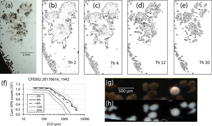
H. L. Bourne et al.: Carbon export and fate beneath a dynamic upwelled filament                                                                               3057

Figure 5. (a) Raw attenuance time series for all CFEs deployed at L2. See Fig. 2 for deployment context. Italicized numbers are the dive
numbers corresponding to the data. The mATN time series scales with flux as timing is constant. (b) Map showing deployment and trajectories
of CFEs, CTD station locations, and tracks of the productivity drifter and sediment trap array during the intensive studies at L2. CFE-1–4 are
indicated by circle, square, triangle, and diamond symbols, respectively. The overlay is the SNPP VIIRS chlorophyll field for 17 June 2017
during the later stages of sampling at this location.

Table 1. Carbon flux explorer deployments during CCE-LTER process study P1706 2 June–1 July 2017.

    Cyclea       Locationb      CFE Name         Deploy UTC           Deploy        Deploy         Deploy         Recovery        Recovery        Recovery
                                                    datec              dayd         latitude      longitude         dayd           latitude       longitude
    1            L1             CFE-2-Cal        20170609            159.9917       35.0739      −121.1281         160.8694        35.0187       −121.1653
    1            L1             CFE-1            20170610            161.1215       35.0000      −121.1686         162.4806        34.9088       −121.2132
    1            L1             CFE-3            20170610            161.0818       35.0000      −121.1686         162.4701        34.9047       −121.1995
    1            L1             CFE-2-Cal        20170611            161.9999       34.9396      −121.2031         162.5528        34.9204       −121.2256
    1            L1             CFE-4-Cal        20170611            162.0197       34.9348      −121.1946         162.5819        34.9061       −121.2074
    2            L2a            CFE-1            20170613            164.1597       34.7391      −121.8349         167.4826        34.9788       −122.4062
    2            L2a            CFE-3            20170613            164.1782       34.7391      −121.8349         167.4972        34.9613       −122.4558
    2            L2a            CFE-2-Cal        20170614            164.9700       34.7771      −122.0572         166.0451        34.8913       −122.3356
    2            L2a            CFE-4-Cal        20170614            164.9822       34.7742      −122.0587         165.9201        34.8850       −122.3084
    2            L2b            CFE-2-Cal        20170616            166.5817       34.7098      −122.3004         167.5375        34.7051       −122.4151
    2            L2b            CFE-4-Cal        20170616            166.5952       34.7091      −122.2998         167.5500        34.7082       −122.4188
    3            L3             CFE-1            20170619            169.9880       34.2382      −123.1001         170.8958        34.1973       −123.0502
    3            L3             CFE-2-Cal        20170619            170.1173       34.2275      −123.1480         170.9007        34.1716       −123.0759
    3            L3             CFE-1            20170621            171.1496       34.1129      −122.9885         172.5139        34.0782       −122.8477
    3            L3             CFE-2-Cal        20170621            171.1150       34.1137      −122.9939         171.9257        34.0773       −122.8891
    3            L3             CFE-4-Cal        20170621            171.1310       34.1086      −122.9823         171.9243        34.0734       −122.8689
    4            L4             CFE-1            20170623            174.1295       34.4032      −123.0964         176.5160        34.4452       −123.0978
    4            L4             CFE-2-Cal        20170623            174.2182       34.4070      −123.0958         174.9417        34.4240       −123.0342
    4            L4             CFE-4-Cal        20170623            174.1028       34.4024      −123.1040         174.9174        34.4294       −123.0595
    4            L4             CFE-2-Cal        20170625            175.0991       34.4218      −123.0168         176.5340        34.4521       −123.0161
    4            L4             CFE-4-Cal        20170625            175.1102       34.4221      −123.0133         176.5132        34.4835       −122.9888
   a CCE-LTER cycle number. b Location number used in this paper. c Deploy date (YYYYMMDD). d Day – year days since 1 January 2017 00:00 UTC. 1 January 2017 at
   12:00 UTC = 0.5.

https://doi.org/10.5194/bg-18-3053-2021                                                                           Biogeosciences, 18, 3053–3086, 2021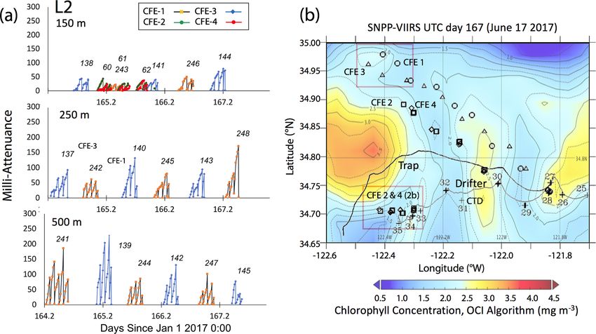
3058                                    H. L. Bourne et al.: Carbon export and fate beneath a dynamic upwelled filament

2.2.2   Conversion of volume attenuance to POC flux               Method 1 – threshold variation

Volume attenuance (VA) has been calibrated in terms of par-       Bourne (2018) developed a computationally efficient nearest-
ticulate organic carbon and nitrogen (POC and PN) loading         neighbour particle detection algorithm to measure attenu-
(Bourne et al., 2019). VA is converted to volume attenuance       ance size distributions in CFE images. This was an impor-
flux (VAF) by normalizing VA by deployment time and scal-         tant first step towards fully autonomous observations as this
ing by the area of the funnel opening. The regression for         scheme can run aboard the CFE. Unlike the “stage” inte-
measured POC flux (mmol C m−2 d−1 ) against VAF (mATN-            gration (Sect. 2.2.1), particle size analysis requires a choice
cm2 cm−2 d−1 ) is given by Eq. (2) (Bourne et al., 2019).         of an attenuance count threshold to distinguish particles and
                                                                  differentiate them from background. Choosing too low of a
POC flux = 0.965 ± 0.093 · VAF                                    threshold can increase the false detection of particles due to
          − 1.1 ± 1.5 mmol C m−2 d−1                       (2)    imperfections of lighting and sensor noise. Bourne (2018)
                                                                  studied thresholds from 0.02 to 0.20 attenuance units. Even
VAF is ∼ 4 times more precisely determined than POC flux          at the highest threshold setting, the method failed to sepa-
(Bourne et al., 2019), and thus we use it as the x-axis vari-     rate touching 250 µm ECD ovoid faecal pellets (Fig. 6) which
able. The regression R 2 = 0.897 and the ± values denote 1        constituted a significant component of particle flux at 150 m
standard deviation of slope and intercept, respectively. For      at L2. In this method, as well as method 3 (below), particle
simplicity, we use a conversion factor of 1.0 to scale VAF        size distributions were determined in the last image of a cy-
to POC flux. The intercept is not significantly different from    cle before the imaging stage was cleaned. If overlapping par-
zero and is ignored. The CFE-derived optical proxy for POC        ticles were present, the previous image in the series would
flux is referred to as POCATN flux below.                         be used instead. This choice was made manually but could
                                                                  be automated. Bourne (2018) used a threshold attenuance of
2.2.3   Particle size distributions                               0.12 to systematically analyse 143 image cycles using this
                                                                  method.
Three methods were used to determine particle size distribu-
tions in CFE imagery: (1) a computationally efficient code        Method 2 – manual counting
that measures particle area and attenuance (Bourne, 2018),
(2) manual identification and counting of particle classes, and   CFE images from L2 were manually enumerated for ovoid
(3) a hybrid of image analysis and visual verification of iden-   faecal pellets and > 1000 µm sized aggregates using a com-
tified particles.                                                 bination of transmitted light and dark-field imagery (Connors
    Transmitted light images from the CFEs were processed         et al., 2018; Bourne et al., 2019).
to attenuance units following Bishop et al. (2016). Results
were saved as imagery in attenuance units where counts            Method 3 – ImageJ size analysis and secondary
in each 8-bit (red, green, blue) colour plane are scaled so       processing
that 100 counts = 1 attenuance unit. The complete set of
1600 CFE transmitted light images and corresponding atten-        In method 3, the software package ImageJ 1.52 (IJ, National
uance images are available through the Biological and Chem-       Institutes of Health) was used for particle size analysis. The
ical Oceanography Data Management Office (BCO-DMO) at             advantage of ImageJ is that the analysis provides a rich statis-
the Woods Hole Oceanographic Institution (Bishop, 2020a).         tical description of the individual particles that can be used
    For size analysis, the RGB image is converted to an 8-bit     to aid in particle class analysis. In this method, we manu-
grayscale image. The 5 MP SUMIX imager used in the CFE            ally inspected the four to five sequential attenuance images
employs a Bayer filter that allocates in a checkerboard pattern   taken during each image cycle to determine the point of on-
50 % of the pixels to green and 25 % to each of the blue and      set of particle overlap. The attenuance image was subtracted
red colour channels. In the case of transmitted light imagery,    from the preceding attenuance image of the clean sample
we have found little difference in attenuance values from the     stage. A threshold of four counts (0.04 ATN) and above was
three colour planes (Bourne et al., 2019); however, this is not   used to define the presence of particles (two counts higher
true of imagery in dark-field illumination. We choose to set      than used for calculation of VA). At this threshold setting,
the definition of a “particle” as having 4 contiguous pixels      large aggregates were fully detected; however, touching par-
above threshold in order to provide compatibility with inter-     ticles – particularly 200–400 µm sized faecal pellets (Fig. 6)
pretation of dark-field imagery, where colour is important.       were not separable. Each IJ-identified “particle” with multi-
A 4-pixel particle has an area of 676 µm2 or an equivalent        ple identical units was counted, and these counts were as-
circular diameter (ECD) of 29 µm.                                 signed to its sequence number. Inspection of the imagery
                                                                  also identified touching large aggregates which were sim-
                                                                  ilarly treated. During secondary data processing, the area
                                                                  of each multi-unit “particle” was divided by the number of

Biogeosciences, 18, 3053–3086, 2021                                                  https://doi.org/10.5194/bg-18-3053-2021
H. L. Bourne et al.: Carbon export and fate beneath a dynamic upwelled filament                                                       3059

Figure 6. (a) Segment of a CFE-2 transmitted light image June 2017 at 19:42 UTC; depth 150 m. (b–e) ImageJ particle outline maps at
attenuance thresholds of 0.02, 0.04, 0.12, and 0.20, superimposed on the attenuance image for the sample. Darker greys denote higher
attenuance. We found that touching faecal pellets could not be separated even at a threshold of 0.20 ATN. At thresholds > 0.06, large
low-density aggregates are seen as highly fragmented, and the contribution of smaller particles is reduced. (f) Particle size attenuance
count distributions as a function of threshold. (g) Magnified image under dark-field illumination. Olive-coloured faecal pellets are readily
distinguished from an unidentified egg. (h) Attenuance map of the same view.

subunits, and its particle number was changed from 1 to                    Figure 7 displays normalized cumulative size distributions
the determined count. Examples of touching ovoid parti-                 prior to and after secondary processing for all CFE dives
cles are found in Fig. 6. Living organisms rarely appeared              at L2. The point of this labour-intensive computer-aided ap-
in images; when they did appear, we were able to identify               proach was to provide a basis for future code development.
pteropods, amphipods, copepods, siphonophores, acantharia,              The scientific outcome of this analysis is a description of the
radiolaria, and foraminifera. These “living” particles were re-         number and attenuance fluxes of differently sized particles
moved from the secondary processed data. Total particle at-             and how these fluxes change down the water column during
tenuance (average particle attenuance times particle area) and          the CCE-LTER process study.
particle number were binned into 65 logarithmically spaced
size categories from (30 to 20 000 µm). A total of 267 im-              Method intercomparison
age pairs were analysed; these combined flux results for each
of 89 CFE dives are available online through the Biologi-               Figure A4 compares normalized-cumulative-attenuance flux
cal and Chemical Oceanography Data Management Office                    and normalized-cumulative-number flux size distributions
(BCO-DMO; Bishop, 2020b). Float CTD results are simi-                   from methods 1 and 3 at locations L1–L4. Some differences
larly archived (Bishop, 2020c).                                         are attributed to independent choices of which image sets to
   Data from each image cycle were weighted by the to-                  analyse (137 vs. 267) using the two methods; nevertheless,
tal number of images in that cycle; data from the multi-                we found good agreement between the methods for data from
ple imaging–cleaning cycles during a dive were binned and               250 m and deeper. The poorer agreement in size distributions
weighted by the duration of each imaging cycle. The par-                from 150 m is due to the high threshold (0.12 attenuance) of
ticle attenuance and number-size-binned data were scaled to             method 1 failing to detect large aggregates as whole parti-
convert results to flux units (mATN–cm2 cm−2 d−1 and num-               cles and also the problem of touching faecal pellets, which
ber m−2 d−1 ). The partitioning of particle flux by size was            dominated samples at 150 m at L2 (Fig. 6).
simplified to five size categories: 30–100, 100–200, 200–                  Figure 8 compares profiles of aggregate (> 1000 µm) and
400, 400–1000, and > 1000 µm. In the process, ATN and                   pellet (200–400 µm) number fluxes with manually deter-
number fluxes at category boundaries were determined by                 mined counts of these classes at location L2. Although the
interpolation of the detailed cumulative flux–size distribu-            data were calculated in slightly different ways, method 3 ag-
tions. The 200–400 µm bin was primarily populated by the                gregate flux and manually determined aggregate flux closely
numerous ovoid pellets. The > 1000 µm bin was dominated                 matched. The method 3 pellet flux agreed closely with man-
by aggregates.                                                          ual counts at 150 m but overestimated results at 500 m by a
                                                                        factor of 5. To understand this difference, we graphed par-

https://doi.org/10.5194/bg-18-3053-2021                                                          Biogeosciences, 18, 3053–3086, 2021
3060                                       H. L. Bourne et al.: Carbon export and fate beneath a dynamic upwelled filament

Figure 7. Processed size distribution data for CFE-1–4 deployed near 150 m at L2. Normalized cumulative attenuance flux is plotted against
equivalent circular diameter (µm). (a) Original cumulative attenuance size distributions from ImageJ and (b) after secondary processing to
correct for touching particles (see insets in upper right-hand corners of a and b). Boundaries for reduced size categories are 30–100 (not
shown), 100–200, 200–400, 400–1000, and > 1000 µm and are indicated in (a) and (b). Open and closed symbols denote data from the
first and second deployments of the CFE-Cals at location 2 designated as L2a and L2b, respectively. After correction, the 400–1000 µm size
category contributed little to sample attenuance.

ticle attenuance for all 150–400 µm sized particles at 150 m           As we show below that the large aggregate size fraction dom-
at L2. Results showed a cluster of particles > 200 µm in size          inates total POCATN flux, it is also true that this flux is de-
with attenuance values > 0.25, which suggested that the clus-          termined by a relatively small number of aggregates arriv-
ter was due to ovoid faecal pellets. We calculated the ratio of        ing during each image cycle. We assume Poisson counting
the number of particles > 0.25 attenuance to total particles           statistics, where the relative√
                                                                                                     standard deviation (RSD) count-
and used the ratio to correct the method 3 counts. Results             ing error for n particles is n/n, and that the RSD can be
brought the method 2 and method 3 counts at L2 into agree-             applied to both number flux and attenuance flux. Figure A5a
ment (Appendix A, Table A1). We applied this approach to               shows representation of this error for the 200–400 µm and
L1, L3, and L4 data (Fig. 8). L4, in particular, showed high           > 1000 µm categories; two cases are calculated: that for in-
numbers of particles in the 200–400 µm category which orig-            dividual dive results and that for the grand average of all
inated from the fragmentation of large low attenuance aggre-           dives at four depth horizons at each location. Count-related
gates; only 15 % of particles had attenuance above 0.25 at             errors for individual dives for the 200–400 and > 1000 µm
250 and 500 m.                                                         categories were typically < 10 % and < 30 %, respectively;
                                                                       similarly, for pooled dive results such errors were typically
2.2.4   Sources of uncertainty of POCATN flux                          < 5 % and 20 %. At L3 where fluxes were low, count-related
                                                                       errors for POCATN flux in 200–400 and for > 1000 µm cat-
Calibration studies by Bourne et al. (2019) were restricted            egories were typically 20 % and 40 %, respectively; pooled
to depths near 150 m due to logistical reasons including ship          results gave ∼ 15 % and 30 % errors. Figure A5b illustrates
time, the need for replication of results, and the need for com-       the combined effect of counting error and 9 % calibration
parison of POCATN fluxes with data from surface-drogued                uncertainty for individual dives at L2 and L3 (as plotted in
sediment traps (Sect. 2.4 below) which were restricted to the          Fig. 15a below). These errors are minor compared to the
upper 150 m. We do not believe that this is a major limi-              range of POCATN flux values observed. The complete dive-
tation because samples collected at 150 m covered a wide               averaged data sets with error estimates are available as sup-
range of size distribution and particle types that were also           plemental online material. Note n values used for error cal-
found deeper in the water column. Furthermore, large par-              culation listed in the supplemental data set are not integers
ticles sampled by large-volume in situ filtration show little          due to number fluxes being based on extrapolations to the
shift in organic carbon percentages from the base of the eu-           boundaries of the five size categories.
photic zone to 500 m (e.g. Bishop et al., 1986). For these rea-           We assume for the following discussion that the
sons, we assume that the uncertainty of our present calibra-           VAF : POC flux relationship has a 9 % uncertainty and is in-
tion is ∼ 9 % (± 1 SD; Eq. 2). More calibration sampling is            variant with depth; furthermore, errors due to the statistical
desired.                                                               frequency of particles in different size categories are also
   During review, we were asked to estimate the contribution           deemed a minor influence on our interpretations.
of counting statistics to the uncertainty of POCATN flux for
the > 1000 µm particle class vs. that for smaller size classes.

Biogeosciences, 18, 3053–3086, 2021                                                        https://doi.org/10.5194/bg-18-3053-2021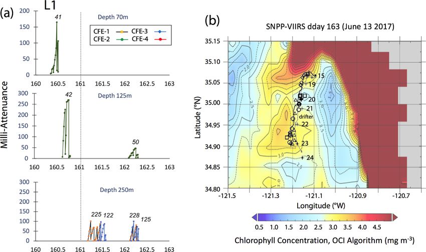
H. L. Bourne et al.: Carbon export and fate beneath a dynamic upwelled filament                                                         3061

Figure 8. (a) Profile of aggregate and pellet number fluxes determined by method 3 and by manual counting at Location L2. The small
blue-filled circles represent number flux of 200–400 µm particles with average attenuance > 0.25. These data agree closely with manually
enumerated pellet counts. Method 3 counted more aggregates in the shallowest samples because the manual method was unable to infer
weakly defined boundaries of less dense aggregates. Data are tabulated in Appendix A, Table A1. (b) Plot of average particle attenuance vs.
equivalent circular diameter (ECD). The red dashed line denotes the lower boundary of the cluster of > 0.25 ATN particles. (c) Profiles of
200–400 µm total particle number fluxes and for > 0.25 ATN particles at L1, L3, and L4. Dashed lines are Martin fits to the ovoid pellet class
fluxes. In all cases, fluxes of faecal pellets decrease with depth.

2.3   Acoustic Doppler current profiler (ADCP) and                          Transmissometer-derived beam attenuation coefficient
      other CTD data                                                     (m−1 ) multiplied by a factor of 27 is used to calculate par-
                                                                         ticulate organic carbon (POC) concentration (µM; Bishop
Current velocity in u (east positive) and v (north positive)             and Wood, 2008). The Seapoint fluorescence data were off-
components from the hull-mounted RD instruments 150 kHz                  set by subtraction of 0.05 units, and residual values lower
narrowband acoustic Doppler current profiler (ADCP) were                 than 0.02 were determined to be below detection. The CTD–
averaged over 30 min intervals during the times of CFE de-               rosette also carried an underwater vision profiler particle
ployment. The 150 kHz data were limited to the upper 400 m.              imaging system (UVP5-hd; Hydro-Optic, France) capable
CFE drift velocities were calculated based on CFE dive loca-             of resolving particles > 64 µm in reflected light. Data are
tions and times. Combined ADCP and CFE drift results are                 archived at https://ecotaxa.obs-vlfr.fr/part/, last access: De-
shown in Fig. 9.                                                         cember 2018, under the project UVP5hd CCELTER 2017.
   The hydrographic context for our study was provided by                We used the “non-living” particle concentrations averaged
CTD profiles of T , S, potential density anomaly (σθ ), pho-             over 5 m, which were representative of particles present in
tosynthetically active radiation (PAR), chlorophyll fluores-             ∼ 180 L. We pooled and further depth-averaged all CTD cast
cence (Seapoint Sensors Inc.), turbidity at 810 nm (Seapoint             data at each location to achieve an equivalent water volume
Inc.), and transmission at 650 nm (WET Labs, Inc. Philo-                 of ∼ 2000 L to improve the statistics of the number concen-
math, OR). Particle optics were kept clean as detailed in                trations of > 1000 µm aggregates. In this paper we focus on
Bishop and Wood (2008). The CTD–rosette casts were usu-                  the > 1000 µm fraction, although all size fractions have been
ally made in close proximity to a surface-drogued produc-                treated identically. Further detailed analyses of UVP5 im-
tivity array which served as the Lagrangian reference for                agery are beyond the scope of the paper.
studies at each location. Nutrient data from the CTD–rosette
samples used in this paper are archived in the CCE-LTER
data repository (https://oceaninformatics.ucsd.edu/datazoo/
catalogs/ccelter/datasets, last access: July 2018).

https://doi.org/10.5194/bg-18-3053-2021                                                           Biogeosciences, 18, 3053–3086, 2021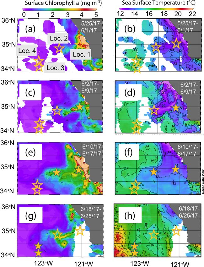
3062                                         H. L. Bourne et al.: Carbon export and fate beneath a dynamic upwelled filament

Figure 9. The 30 s averaged current velocities in u (east positive) and v (north positive) directions from 150 kHz narrow band ADCP data.
CFE depths during flux measurements are shown. Profiles denoted by black asterisks to right of each contour plot are averaged ADCP
velocities for the entire time span. Red points represent average CFE velocities over the course of each dive. Shaded boxes denote missing
data. Filled blue triangles are the averaged CFE velocities for all dives at a given depth. Panels (a), (b), (c), (d), and (e) Locations 1, 2a, 2b,
3 and 4 respectively.

2.4    New-production-based carbon export (POCNP flux)                      150 m are from Stukel and Landry (2020). These values are
       and particle interceptor trap flux                                   referred to as POCPIT flux.
                                                                               In this study, CFEs were programmed to dive deeper than
                                                                            100 m, and POCATN fluxes were lower than POCNP values
Euphotic zone new production (NP) measurements at loca-
                                                                            at all locations except at L4, the last occupation of the fila-
tions L1, L2, L3, and L4 (converted to carbon units) were
                                                                            ment; in this case POCATN flux exceeded POCNP by a factor
189 ± 21, 156 ± 77, 63 ± 33, and 19 ± 3 mmol C m−2 d−1 ,
                                                                            of > 2 at 250 m, suggesting a recent decline in carbon ex-
respectively (Kranz et al., 2020). We refer to these data
                                                                            port. Nitrate and beam attenuation coefficient (POC) changes
as POCNP flux. POC fluxes from deployments of surface-
                                                                            (Table 2) allow an estimate POCNP flux for the 9 d interval
drogued particle interceptor traps (PITs) traps deployed to

Biogeosciences, 18, 3053–3086, 2021                                                              https://doi.org/10.5194/bg-18-3053-2021
H. L. Bourne et al.: Carbon export and fate beneath a dynamic upwelled filament 3063
3 Results
3.1 Spatial context and water column environment
CFE deployment locations and times are summarized in
Table 1 (above). Table 2 summarizes mixed-layer and eu-
photic zone properties for each intensive study location. Fig-
ures A1b, 5 (above), A2b, and A3b show satellite-retrieved
surface chlorophyll fields from SNPP VIIRS with superim-
posed locations of CFE surfacing and CTD/optics profiles
and tracks of the surface-drogued particle interceptor trap
(PIT) array and of the drogued productivity (PROD) array at
locations L1–L4, respectively. At locations L1 and L4, the
Lagrangian CFEs tracked well with all deployed systems;
at L2, there was a divergent behaviour of CFEs, PIT, and
drifters with the CFE and PIT arrays remaining closest; at
L3, the CFE and PIT arrays maintained a similar track. At
all locations, CFE trajectories closely matched ADCP veloc-
ities (Fig. 9) and the patterns of flow suggested by sea surface
altimetry (Fig. 4).
Figure 11 shows time series depth plots of T , S, poten-
tial density (σθ ), chlorophyll fluorescence, transmissometer-
derived POC, and turbidity at locations L1 through L4. Fig-
ure 12 shows time series POC and S versus potential density
plots at L1 through L4 as well as spatial transects of POC and
Figure 10. Profiles of averaged T , S, potential density, beam atten-
salinity versus potential density. We reordered the time axis
uation coefficient (650 nm), and nitrate in the upper 150 m at loca- in these figures to make data from in-filament locations L1,
tions L1, L2a, L2b, L3, and L4. Error bars are ± 1 SD. L2, and L4 more logically related and separate from the out-
of-filament transitional waters at L3. L2 is split temporally
into L2a and L2b for reasons outlined below.
spanning the occupations of L2 and L4. We have confidence
in this calculation since a sediment trap array, deployed late 3.1.1 Location 1
in the study at L2b, tracked the water to L4 (Kranz et al.,
2020); furthermore, L2b and L4 salinity profiles were vir- The study site L1 was located in the middle of a 50 km wide
tually identical (Fig. 10), confirming that the surface water 500 m deep trough (Fig. 2) approximately 25 km offshore of
masses encountered at L2 were nearly the same as at L4. Morro Bay, CA. The SNPP VIIRS chlorophyll (Fig. A1b)
Following Johnson et al. (2017), we subtract 0–45 m stocks shows that early CFE and CFE-Cal deployments took place
of dissolved nitrate at L2b from L4 (Table 2) and multiply in close proximity to very-high-chlorophyll waters. Up-
this change by the molar ratio of photic layer plankton C/N. welling was active as evidenced by cold, high-salinity sur-
Johnson et al. (2017) used a C/N ratio of 6.6; we used a C/N face waters and low stratification (Figs. 10, 12). The 24 h
of 6.4 (Stukel et al., 2013). We chose 45 m as the integration mixed-layer depth (MLD24 ), defined by a potential density
depth as dissolved nitrate profiles at the two sites converged increase of 0.05 kg m−3 relative to surface values (Bishop
at this depth (Fig. 10) and also because 45 m was close to the and Wood, 2009), averaged 19 m (range from 13 to 25 m) and
euphotic zone depth at L4. The calculation yielded an aver- matched euphotic zone depth (16 ± 4 m) (Table 2). Mixed-
aged POCNP flux = 111.3 ± 32.2 (SD) mmol C m−2 d−1 over layer nitrate dropped from 10.2 to 5.4 µM over several days.
9 d, similar to measured POCNP at L2, but a factor of 6 higher CFE attenuance time series showed an early high flux event
than reported at L4 by Kranz et al. (2020). POC inventory (Fig. A1a). ADCP-derived currents (Fig. 9a) show strong
changes (Table 2) from L2b to L4 between the two times im- tidal fluctuation; however, there was a net southwest trans-
plied an average POC loss rate of 33 mmol C m−2 d−1 . Crus- port of water in the upper 50 m at a velocity of 0.06 m s−1 ,
tacean grazers have assimilation efficiencies of 70 %, with at 0.02 m s−1 between 100 and 200 m, and at 0.04 m s−1 be-
the remaining fraction voided as faecal pellets. Export from tween 200 and 300 m. Deployed instrument trajectories were
this POC loss would add ∼ 10 mmol C m−2 d−1 . Averaged consistent with ADCP results.
export from L2b to L4 sums to ∼ 120 mmol C m−2 d−1 .
https://doi.org/10.5194/bg-18-3053-2021 Biogeosciences, 18, 3053–3086, 20213064 H. L. Bourne et al.: Carbon export and fate beneath a dynamic upwelled filament
Table 2. Hydrographic and euphotic zone properties at CCE-LTER P1706 study locations.
Location Mean MLD zeu zeu zeu Mean σθ @ Mean Mean Stock Stock
MLD24 range (SAT) (PAR) (PAR) 0–20 m euphotic 0–20 m 0–20 m 0–45 m 0–45 m
(m) (m) (m) (m) range NO3 base salinity cp POC NO3
(m) (µM) (kg m−3 ) (PSU) (m−1 ) (mmol m−2 ) (mmol m−2 )
1 19 13–25 21 19 16 ± 4 7.76 25.5 33.748 0.943 685.8 625 ± 59
2a 26 18–36 29 25 25 ± 3 8.02 25.5 33.637 0.763 557.5 616 ± 19
2b 26 18–36 29 25 25 ± 3 7.82 25.5 33.636 0.454 410.2 522 ± 26
4 9 5–14 – 51 51 ± 6 3.15 25.0 33.595 0.159 111.1 371 ± 18
3 27 11–69 77 49 49 ± 7 1.89 25.8 33.160 0.088 103.9 124 ± 18
MLD24 : daily average mixed-layer depth based on σθ difference = 0.05 kg m−3 ; zeu : euphotic zone depth based on satellite (SAT) or CTD photosynthetically active radiation
(PAR) 1 % light level.
Figure 11. (a) Salinity, (b) temperature, (c) sigma theta (σθ ), (d) chlorophyll fluorescence, (e) transmissometer-derived POC, and (f) turbidity
time series from CTD casts. The time axis (in UTC days since 1 January 00:00 2017) has been reordered so that L1, L2, and L4 are grouped.
L3 is shifted to the right side of each panel. The white dashed line and red line (c) and (d) denote averaged 24 h mixed-layer depths and
euphotic zone depths, respectively. The chlorophyll fluorescence (d) depth axis is 150 m; the limit of detection was 0.02 units.
3.1.2 Location 2 aged 0–20 m nitrate was 8.6 and 7.8 µM during 2a and 2b,
respectively; salinity values were identical. Chlorophyll flu-
Site L2 was located 110 km offshore. MLD24 averaged 26 m orescence and transmissometer-derived POC decreased by a
and matched the euphotic zone depth of 25 ± 3 m. The base factor of 2 during observations at 2a and 2b (Figs. 11d and
of the euphotic zone was bounded by the σθ = 25.5 kg m−3 12a). During the later stages of CFE observations, SNPP VI-
isopycnal. The temperature and salinity profiles from CFE- IRS surface chlorophyll fields were almost uniform (1.8 to
1 and CFE-3 (Bishop, 2020c) were in close agreement with 2.5 mg chl a m−3 ; Fig. 5b).
CTD casts 25–30 (locations Fig. 5b), whereas the subsequent CFE-1 and CFE-3 were launched in a fast-moving part of
CTD cast data and CFE-1 and CFE-3 data diverge. The early the filament and transported to the WNW (Fig. 5b) and sep-
CTD casts revealed a stronger halocline and pycnocline, with arated from the surface-drogued PIT array and productivity
saltier, denser waters between about 25 and 150 m, indicat- drifter; 20 h later, CFE-Cals 2 and 4 similarly tracked to the
ing upwelling in this part of the time series (Figs. 10 and WNW on a parallel course to CFE-1 and CFE-3 (Fig. 5b).
11). We thus treat the first six CTD casts as representative When redeployed a day later near the drifter, CFE-Cals 2 and
of CFE deployment 2a and subsequent casts as 2b. Aver- 4 advected to the west but at a greatly reduced speed, indi-
Biogeosciences, 18, 3053–3086, 2021 https://doi.org/10.5194/bg-18-3053-2021H. L. Bourne et al.: Carbon export and fate beneath a dynamic upwelled filament 3065
Figure 12. (a) Transmissometer particulate organic carbon (POC) and (e) salinity – potential density time series during the intensive studies
at L1, L2a, L2b, L4, and L3. Also shown are cross-filament transects T1, T2, and T3 for POC (b, c, d) and salinity (f, g, h). Transect locations
are shown in Fig. 2. Transect T1 (UTC day 158) was located between L1 and L2; T2 (day 168) was sited between L2 and L4; and T3 crossed
the outer edge of the filament on day 174 after completion of work at L4. Distances are in kilometres. UTC days as defined in Fig. 10. The
arrows in (f) and (g) indicate the high-salinity surface water in the filament; its scale was ∼ 5 km wide at T1 and ∼ 25 km wide at T2.
cating that the upper 200 m had become decoupled from the Salinity of the upper 50 m at L3 decreased over time from
faster flow tracked by CFE-1 and CFE-3. During L2a, ADCP 33.35 to less than 33.2 PSU, indicating an increasing compo-
data showed a consistent net west-northwest current velocity nent of the southerly flowing low-salinity California Current
at 0.17 m s−1 in the upper 50 m, an increase to 0.29 m s−1 water (Schneider et al., 2005). Surface layer nitrate averaged
between 100 and 200 m, and 0.27 m s−1 between 200 and 1.9 µM. CFE flux indicators were low (Fig. A3a). Current
300 m (Fig. 9b); CFE motions were used to infer a veloc- flow was to the southeast at L3 with 0.30 m s−1 velocities
ity of 0.15 m s−1 at 500 m. During L2b, the current direc- in the upper 50 m, 0.14 m s−1 between 100 and 200 m, and
tion was to the west, but velocities were reduced at all depths 0.08 m s−1 between 200 and 300 m (Fig. 9d). CFE drift at
(0.04 m s−1 in the upper 50 m, 0.11 m s−1 between 100 and 500 m was 0.07 m s−1 . CFE trajectories followed the path of
200 m, and 0.12 m s−1 between 200 and 300 m; Fig. 9c). the PIT array but at a slower speed.
3.1.3 Location 3
3.1.4 Location 4
L3 was located 240 km offshore in transitional waters be-
tween the westward-extending filament and the surround-
ing southerly flowing waters of the California Current. The This site (235 km offshore) was located ∼ 35 km north of L3
MLD24 at L3 averaged 27 m (range 11–69 m). The euphotic in the western extension of the filament (Fig. 3g, h). Based
zone was at least twice as deep as the MLD24 (77 m NASA on the salinity signature of L2b and L4, the water masses
VIIRS; 49 ± 7 m from PAR profiles, Table 2). The base of were similar (Table 2, Fig. 10). SNPP VIIRS chlorophyll
the euphotic zone was bounded by the σθ = 25.75 kg m−3 data (Fig. A3b) show low and nearly uniform chlorophyll
isopycnal. CFE-1 and CFE-3 and CFE-Cal-2 were launched (0.25 mg m−3 ) in the vicinity of observations. Surface nitrate
but recalled within 24 h for repositioning as CTD cast data was depleted, and sea surface temperature had increased due
indicated a relatively strong influence of the filament. CFE- to solar heating (Figs. 3h, 10). MLD24 averaged 9 m; eu-
3 was lost at this time. CFE-1 and CFE-Cals 2 and 4 were photic depth was 51 ± 6 m. The euphotic zone base corre-
redeployed approximately 10 km to the south of the first de- sponded to the σθ = 25.0 isopycnal. ADCP currents were to
ployment locations. the northeast at 0.11 m s−1 in the upper 50 m, decreasing to
0.04 m s−1 between 100 and 200 m, and 0.02 m s−1 between
https://doi.org/10.5194/bg-18-3053-2021 Biogeosciences, 18, 3053–3086, 20213066 H. L. Bourne et al.: Carbon export and fate beneath a dynamic upwelled filament
by 250 m. At L3, in transitional waters, particles would lag
behind the motion of surface waters by 14 km by 150 m and
lag surface waters by 83 km on arrival at 500 m. At L4, parti-
cles settling at 100 m d−1 would lag behind the 50 m layer by
3.5 km on reaching 150 m and would have a total displace-
ment of 13 km by 500 m.
In summary, inferred lateral displacements were calcu-
lated relative to the direction of flow of surface waters as
particles sink from 50 m to deeper waters. The smallest net
Figure 13. Displacements (in kilometres) in the direction of mo- displacements of sinking particles was found at L1 (7 km,
tion of the filament for particles with a hypothetical sinking rate of 300 m), L4 (13 km, 500 m), and L2a (14 km, 500 m). Loca-
100 m d−1 as they sink from 50 m. Extreme displacements were cal- tion L3 in the transitional waters had the strongest net dis-
culated for transitional waters (L3) where sinking particles lagged placements (83 km) by 500 m, making a 1D interpretation of
behind the surface layer by as much as 85 km. Sinking particles particle flux most problematic at this location. An interesting
would lead the surface layer by 20 km at a depth of 250 m at L2a. feature of L2 is that particles at depth would lead the sur-
Calculated from ADCP velocities in Fig. 9. face layer. Displacements of particles sinking at a different
velocity, V , would scale by 100/V .
Particle flux profiles observed by the CFEs may reflect het-
200 and 300 m; at 500 m, a velocity of 0.03 m s−1 was calcu- erogeneous sources over the scales of displacement. If spa-
lated from CFE drift displacements. tial gradients of particle sources along the axis of the plume
A reasonable assumption is that the average salinity of are weak, then the vertical lead and lag effects will be in ef-
the surface layer (here defined as upper 20 m) at L2 and L4 fect smaller. SNPP VIIRS chlorophyll fields provide a mea-
is a result of binary mixing of recently upwelled L1 wa- sure of mesoscale chlorophyll variability at location L2. Im-
ter with the California Current water at L3. Using data in agery from 14 June during the early stages of sampling show
Table 2, we calculate that surface waters at L2a were an chlorophyll varying over a range of 3 to 1.75 mg chl m−3
81.1 : 18.9 % mixture of L1 and L3 waters; similarly, L2b along the path of the profiling CFEs. Imagery from 17 June
was 80.9 : 19.1 %, and L4 was 74 : 26 %. As the filament showed a variation of 2.5 to 1.75 mg chl m−3 (Fig. 5b) along
moved over 200 km offshore it remained mostly hydrograph- the same track. The two images for 14 and 17 June show
ically distinct. ranges of 2.25 to 2.75 and 1.75 to 2.25 mg chl m−3 , respec-
tively, in the vicinity of the later deployment of CFEs (waters
3.2 Sinking particle lateral displacements referred to as L2b). If chlorophyll is a metric of particle flux,
then spatially variable fluxes would be expected to vary by
One of the questions raised in particle flux measurement is as less than a factor of 2 at L2. Similar maps for L1, L3, and L4
follows: how well are fluxes at depth related to measured sur- (Figs. A1, A2, and A3) indicate the likelihood of heteroge-
face layer export? As an exercise we consider particles sink- nous fluxes at L1 and L3 but minimal heterogeneity at L4.
ing at a hypothetical rate of 100 m d−1 from 50 m to depths
of 150, 250, and 500 m and their lateral displacements dur- 3.3 Particle classes and size-dependent POCATN fluxes
ing sinking at the four locations. Figure 13 visualizes such
displacements. Figure 14 shows representative CFE imagery (selected from
CFE positions followed a near-linear trajectory in time at the 1250 images) taken at the four locations at depths of 70,
many locations despite drifting at different depths; trajecto- 125, and 250 m at L1 and at depths of 150, 250, and 500 m
ries were in close agreement with ADCP current velocities at the other locations. The dominant class of particles con-
(Fig. 9). The linearity of track allows a simple calculation tributing to export at each location varied. Shallow export
of displacements in the direction of motion. At L1, ADCP flux through 100 m at L1 was dominated by 7–10 mm long
velocity data (discussed in Sect. 3.1) indicate that particles optically dense anchovy pellets (Fig. 14); at L2 copepod pel-
sinking at 100 m d−1 would lag behind the surface layer by lets (Figs. 14, 6g, h, 8a) accounted on average for 50% of
7 km as they transited from 50 to 300 m. At L2a, particles the flux (range 10 % to 90 %; Fig. 7b) with > 1000 µm ag-
leaving 50 m would lead the surface layer by 11 km by the gregates (Figs. 6, 14) accounting for the rest. At L3 and L4,
time they arrived at 150 m; they would lead surface waters by export was dominated at all depths by > 1000 µm sized ag-
a total of 19 km by 250 m; particles would lag the 250 m layer gregates. Large > 1000 µm sized aggregates resembling dis-
by 4.5 km on reaching 500 m. Taken together, particles sink- carded larvacean houses were common at all sites at depths
ing from 50 m would have a net displacement of 15 km rela- 250 m and below. We infer their origin based on size and
tive to the surface layer. At L2b, in a weaker current regime, morphology. Such aggregates were also present in samples
sinking particles would lead the surface layer by 6 km during closer to the surface, though not typically as abundant.
transit to 150 m and have a total displacement lead of 12.5 km
Biogeosciences, 18, 3053–3086, 2021 https://doi.org/10.5194/bg-18-3053-2021You can also read