Challenges for machine learning in clinical translation of big data imaging studies
←
→
Page content transcription
If your browser does not render page correctly, please read the page content below
Challenges for machine learning in clinical translation of big data
                                                                      imaging studies
                                                  Nicola K. Dinsdalea,∗, Emma Bluemkeb , Vaanathi Sundaresana , Mark Jenkinsona,c,d ,
                                                                       Stephen M Smitha , Ana I. L. Nambureteb
                                          a
                                            Wellcome Centre for Integrative Neuroimaging, FMRIB, Nuffield Department of Clinical Neurosciences,
                                                                                    University of Oxford, UK
                                              b
                                                Institute of Biomedical Engineering, Department of Engineering Science, University of Oxford, UK
                                          c
                                            Australian Institute for Machine Learning (AIML), School of Computer Science, University of Adelaide,
                                                                                       Adelaide, Australia
                                           d
                                             South Australian Health and Medical Research Institute (SAHMRI), North Terrace, Adelaide, Australia
arXiv:2107.05630v1 [eess.IV] 7 Jul 2021

                                          Abstract
                                          The combination of deep learning image analysis methods and large-scale imaging datasets
                                          offers many opportunities to imaging neuroscience and epidemiology. However, despite the
                                          success of deep learning when applied to many neuroimaging tasks, there remain barriers
                                          to the clinical translation of large-scale datasets and processing tools. Here, we explore the
                                          main challenges and the approaches that have been explored to overcome them. We focus
                                          on issues relating to data availability, interpretability, evaluation and logistical challenges,
                                          and discuss the challenges we believe are still to be overcome to enable the full success of
                                          big data deep learning approaches to be experienced outside of the research field.
                                          Keywords: Neuroimaging, Deep Learning, Clinical Translation

                                          1. Introduction

                                                  Across neuroimaging, the majority of datasets have been limited to small-scale collec-
                                          tions, typically focusing on a specific research question or clinical population of interest.
                                          Recently, however, large scale ‘big data’ collections have begun to be collated, many of
                                          which are openly available to researchers, meaning that, if the acquisition protocol, de-
                                          mographic and non-imaging information of the data meets the requirements of the study,
                                          novel research can be completed without having to acquire new scans. The sharing of these
                                          large-scale datasets has had many benefits: not only do they enable the exploration of new
                                          research questions, they also enable reproducibility and quicker method prototyping.

                                              ∗
                                                  Corresponding Author - nicola.dinsdale@dtc.ox.ac.uk
                                          Preprint submitted to Neuron                                                              July 14, 2021
Existing large-scale datasets have been curated to explore different research questions
with varying numbers of subjects and imaging sites across studies. For instance, if the
research question were about lifespan and ageing, datasets to consider would include: IXI1
(n = 581), NKI-RS (Nooner et al., 2012) (n > 1000), UK Biobank (Sudlow et al., 2015)
(n = 100, 000), CamCAN (Taylor et al., 2017) (n = 700) and Lifespan HCP in Ageing
(Bookheimer et al., 2018) (n > 1200). Similarly, if one was interested in early development,
available datasets include: dHCP (Hughes et al., 2017) (n > 1000) and ABCD (Marek
et al., 2019) (n > 10, 000), or for research on young adults, one could consider: HCP Young
Adult (Van Essen et al., 2013) (n=1200), GSP (Holmes et al., 2015) (n = 1070) and CoRR
(Zuo et al., 2015) (n = 1629). Datasets also exist that explore specific clinical groups, such
as Alzheimer’s (OASIS 3 (Marcus et al., 2007) (n = 1098) and ADNI (Jack et al., 2008)
(n > 3500)), Autism (ABIDE (Di Martino et al., 2013) (n = 1112)), and schizophrenia
and bipolar disorder (CANDI (Frazier et al., 2008) (n = 103)). These datasets allow the
exploration of questions that would not be possible with traditional small-scale studies where,
for instance, the statistical power would not be sufficient to find significant results. For
instance, if we are interested in exploring individual differences from the average trajectory
rather than differences within-subject or group, we are likely to require a larger sample size
afforded by the large-scale datasets (Madan, 2021). Large-scale studies have also enabled the
characterisation of potential subtypes within patient samples – for example, (Young et al.,
2018) demonstrated heterogeneity and subtypes in atrophy patterns due to Alzheimer’s
disease using data from ADNI.
      UK Biobank (Sudlow et al., 2015) is the largest of these studies, with a goal of collecting
brain imaging data from 100,000 volunteers, including 6 MRI modalities, to study structure,
function, and connectivity. UK Biobank also contains large quantities of lifestyle, genetic
and health measures, which allow researchers to create models of population ageing and
model how genetic and environmental factors interplay with this process. For instance, the
atrophy of the hippocampus is a well-validated biomarker for Alzheimer’s disease, and so,
using the UK Biobank, a nomogram of hippocampal volume with normal ageing has been
created (Nobis et al., 2019), illustrating the progression with age and percentiles of expected
volume across the population.
      For population-based models to have maximal impact they need to be translatable – that
is, they need to have genuine clinical impact beyond the research field. Having created a
model of healthy ageing, when a patient arrives in the clinic we wish to be able compare

  1
      https://brain-development.org/ixi-dataset
                                                 2
their MRI scan to normative distributions. This would then allow us to identify whether the
patient was ageing differently to the population average, and potentially identify the need
for intervention. Unfortunately, comparing a scan to the normative model is not as simple
as merely acquiring a scan and making that comparison. First, research data differs from
clinical data in terms of quality, acquisition and purpose and, further, MRI data acquired on
different scanners or with different protocols may differ in characteristics to such an extent
that comparisons with the model are no longer valid. These ‘batch effects’ also cause a
harmonisation problem within many large studies, where data collected on different scanners
within the study contain bias introduced by the effects of the particular scanner hardware
and acquisition protocol on the image characteristics. Second, the populations may differ so
much that the patient falls outside of the population modelled, and it cannot be known if the
models will extrapolate. For instance, as UK Biobank spans subjects from 45-85 years of age,
any model developed on this data is unlikely to extrapolate well to subjects much younger
than that range. Third, logistical challenges make the deployment of the models difficult in a
clinical setting, potentially to the point where it is not currently possible for them to be used
outside of the research world, for instance the dependence on GPUs for processing which are
unlikely to be available. Further, many research studies utilise functional and diffusion MRI
which are often unavailable clinically due to the lack of expertise and equipment, and long
acquisition times being impractical (e.g., to match the quality or time taken over research
scans). Functional connectivity analyses, for instance, have become a prominent approach
for examining individual differences, driven by the availability of high quality data from the
large-scale studies. Ultimately, if this data cannot be acquired clinically, the utility of any
model is limited. Solutions to these problems, however, are beginning to be developed and
deep learning offers potential opportunities.
   Due to the growth in size of the datasets, deep learning models are now an option
for neuroimaging analysis, enabling us to explore new questions in a data-driven manner.
Applications of deep learning techniques to neuroimaging data have been explored in a
research setting, with increasing numbers of novel methods proposed year on year. Powered
by their ability to learn complex, non-linear relationships and patterns from data, deep
learning methods have been applied to a wide range of applications and have found success
in previously unsolved problems. However, challenges for applying deep learning models to
the clinical domain remain. These challenges limit the impact that big datasets such as the
UK Biobank are currently able to have on patient care, and work must be undertaken to
allow models to extend beyond the research domain. Recent developments in deep learning

                                                3
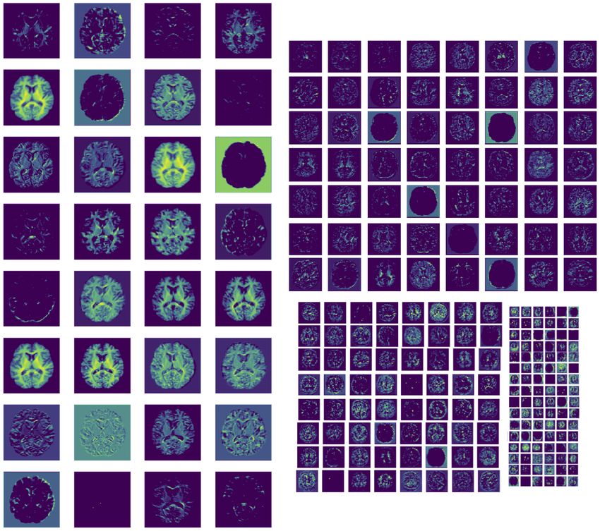
Figure 1: An example network architecture for a convolutional neural network (CNN) for a classification or
regression task.

have begun to tackle the problems faced, but further developments are needed. Here, we
will discuss the challenges being faced and current approaches being developed to mitigate
them, covering challenges around data availability, interpretability, model evaluation and
logistical challenges including data privacy. We will also identify and explore the barriers
we believe still need to be overcome.

1.1. Deep Learning Background
    To understand the challenges for clinical translatability of deep learning methods, we
first require an overview of how these methods approach problems – for a more detailed in-
troduction see, for example, (LeCun et al., 2015). We will only consider convolutional neural
networks (CNNs), which form the vast majority of deep learning methods currently applied
in medical imaging, an example architecture of which is shown in Fig. 1. The majority are
supervised approaches (LeCun et al., 2015), meaning that to explore the research question,
we need access to a dataset of images, X, and the set of known true labels, y, for the task
we wish to explore. This requires an understanding of the information that we expect to be
encoded within the images and an understanding of which questions are of interest, defined
as domain knowledge. Examples for the X and y data could be a structural scan with an
associated segmentation mask, or multiple modality data for X, with the label being disease
prognosis.
                                                    4
Having curated and appropriately preprocessed the data (for instance, skull stripping,
bias field correction, see e.g. (Manjón, 2017)) the task is then to design a neural network
architecture which we expect to be able to map from X to y through learning a highly
non-linear mapping function f (X, y; W ), where W are the trainable weights of the neural
network. The choice of architecture is highly influenced by a variety of factors: the task
being explored, the quantity of data available, and the computational power available, and
is again highly influenced by domain knowledge.
   Nevertheless, most networks are formed through the same basic building blocks. The
first are convolutional filters, which learn features of interest from the data, encoding spatial
relationships between pixels by learning the image features from small patches of the input
data, determined by the filter’s kernel size. These layers, then, complete feature extraction.
They contain the weights and biases which need to be learned during the optimisation
process, W = {w, b}, and stacks of these layers are placed at different spatial resolutions in
order for a range of different features to be extracted at each level of abstraction, allowing
us to create a rich understanding of the input data. During the forward pass of the back
propagation training procedure (LeCun et al., 1990a), each filter is convolved across the
width and height of the input volume. This means that the network learns filters which
activate when specific features are detected, and the exact nature of the features is learned
through a network optimisation procedure that updates the filter weights, in order to find
features that are useful contributors to the overall goal of predicting y.
   The next components are the activation functions which play a fundamental role in the
model training. The activation functions apply a non-linear transformation to the data,
after it has been weighted by the convolutional layers. This non-linearity provides a distinct
edge to CNNs, allowing them to learn the complex non-linear relationships (or mapping)
between the input and the output. Without the non-linear activation functions, CNNs would
be rendered as only linear models, despite the flexibility to learn the weights. Commonly
used activation functions include rectified linear units (ReLU, e.g., zeroing negative values
and keeping positive ones unchanged) (Glorot et al., 2011) and sigmoid (e.g., squashing
large values down to ceilings). Therefore, the features, zl , at layer depth l are given by
zl = ReLU (z(l−1) ∗ wl + bl ) and we can see that, due to the CNN’s sequential data flow,
the features at a given depth are a non-linear combination of the previous features and the
weights and biases. Therefore, despite the sequential nature of CNNs, without the activation
functions we would only be able to train linear models. Example extracted features, zl , after
the activation function, can be seen in Fig. 2.

                                               5
Figure 2: Example extracted features, zl , for brain age prediction (see (Dinsdale et al., 2021a)) at different
network depths and spatial resolutions. It can be seen that several different features are extracted and some
features are repeated, showing redundancy in filters.

                                                        6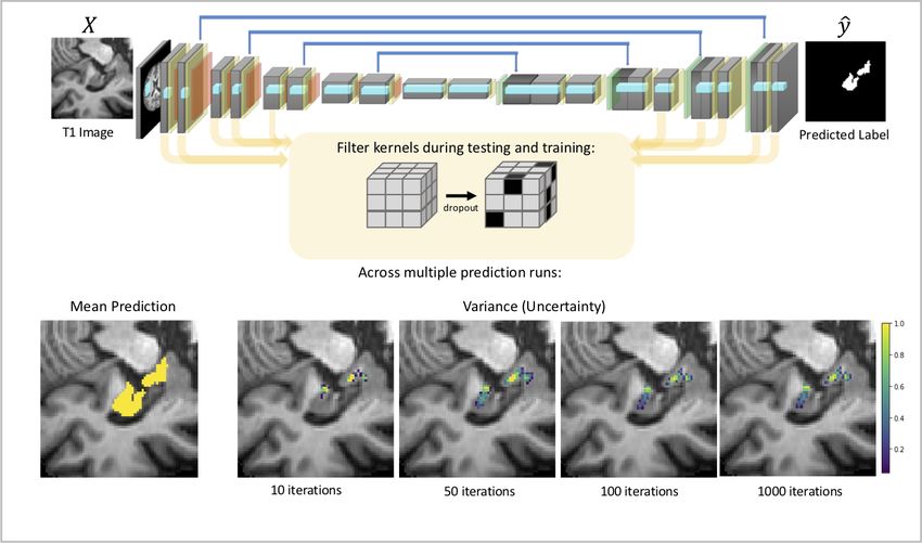
The networks then learn features at different spatial resolutions through the inclusion
of pooling blocks, which reduce the input over a certain region to a single value, thus sub-
sampling the data and condensing information. Pooling condenses the intensity-based infor-
mation, provides a basic invariance to rotations and translations, and has been demonstrated
to improve the object detection capability of convolutional networks. Learning features at
different resolutions allows the network to create a rich understanding of the input image,
aiding the mapping between the input data, X, and the output label, y.
   The final key components of neural networks are fully connected layers, which are essen-
tial to many classification or regression architectures. They are normally placed at the end
of a network, after the convolutional layers have extracted features from the data, and then
the fully connected layers learn how to classify these features. The activation map from
the final layer of the feature extraction is reshaped into a long vector instead of a volume
tensor. In fully connected layers, all nodes in one layer are connected to all the nodes in
the next, meaning that they are much more computationally powerful and expensive than
convolutional layers.
   By feeding the data through the network, we are able to create an output prediction.
To make these predictions accurate, the weights of the network must be optimised using a
process called back propagation (LeCun et al., 1990a), and normalisation techniques such as
batch normalisation are added to minimise the impact of outliers and help result generali-
sation (i.e. performance on new or unseen datasets)(Ioffe and Szegedy, 2015). To this end,
we evaluate a loss or cost function which determines the error in the network prediction
by comparing the prediction (ŷ) and the true label (y). The choice of the loss function is
task-dependent, and plays a crucial role in the final network performance. The optimisa-
tion algorithm is often stochastic gradient decent or a similar algorithm, which updates the
weights such that we reach a minimum in the loss space: that is, a model which minimises
the loss. The aim is to find the global minimum of the loss space, which is the place in
the loss space which most minimises the loss function. However, the optimisation can get
stuck in local minima, which are spots of low loss due to the non-convex nature of the loss
function, and so the learning rate (the step size taken during the optimisation process) must
be chosen to best help the model find the global minimum.
   Therefore, we have an optimisation problem, the performance of which is highly depen-
dent on two factors: first, the design decisions made about the network architecture and
the loss function; second, the data available to train the network. This optimisation pro-
cess determines the location of the decision boundary, that is which locations in the feature

                                             7
Figure 3: When Learning to classify samples (e.g., pixels or subjects - circles and squares), there is likely to
be a continuum between the classes and the decision boundary chooses where one class begins and another
ends. For subjects close to this decision boundary, it becomes critical as it determines the classification
given.

space will be allocated to which class and so which data points are allocated to each class,
as illustrated in Fig. 3.
    In computer vision, where most of the deep learning techniques have been developed,
very large datasets are available, with datasets commonly consisting of many millions of
data points (e.g., 2D training images with labels), and being relatively easy to curate, for
instance, by scraping the internet for images. In neuroimaging in general, data has to
be labelled by a domain expert rather than mechanically produced. This is one of many
differences between working in medical imaging and the general computer vision field, and
therefore, although many of the methods used were developed in vision-related fields, there
are challenges specific to working in the medical imaging or neuroimaging domain.

2. Data Availability

    For clinical translatability of deep learning techniques, data availability is a major limi-
tation. Despite the growth in the size of available datasets, the largest are still only of the
order of tens of thousands of imaging subjects, with a thousand images being commonly
regarded as a large dataset. For many specific tasks, datasets exist only in the order of
                                                       8
hundreds of subjects, due to many factors such as the monetary and time cost of acquiring
data, the difficulties in sharing and/or pooling data across sites, and the fact that, for some
conditions, there are insufficient patients to create a dataset of any great size (Morid et al.,
2021). For instance, the frequently explored Brain Tumour Segmentation (BraTS) dataset
(Menze et al., 2014) only has data from 369 subjects2 available for training, which is in
stark contrast to the popular datasets from computer vision such as ImageNet (Deng et al.,
2009) (1,281,167 training examples), CIFAR-10 (Krizhevsky et al., 2009) (50,000 training
examples) and MNIST (Lecun et al., 1998) (60,000 training examples) where many of the
methods are being developed. By simply looking at dataset sizes, it is clear that we are
likely to be underpowered for training neural networks. Highly parameterised, deep neural
networks are very dependent on the amount of available training data (Cho et al., 2015;
He et al., 2020), with performance generally improving as the number of data points is
increased, and they are far more affected by the amount of available training data than
classical machine learning techniques, due to the need to learn the useful features as well as
the decision boundary (He et al., 2020).
2.1. Maximising the impact of available data
There has, therefore, been an increasing focus on developing techniques to facilitate the
most effective use of the data available. A commonly used technique from computer vision
is the use of large natural image datasets (Raghu et al., 2019; Talo et al., 2018; Mehmood
et al., 2021), with ImageNet (Deng et al., 2009) being the most popular (Cheplygina et al.,
2019), to pre-train the network. Pre-training involves training the weights on a related
task with more available data, such that the optimisation starts from an informed place,
rather than a random initialisation. We can see why this might be useful by considering
the information learned by the network at the different stages (Olah et al., 2018): the early
layers learn features such as edges and simple textures, largely resembling Gabor filters – see
Fig. 2 – and are therefore very general and applicable across different images, regardless of
the target tasks (Yosinski et al., 2014). The deeper convolutional layers then tend to learn
features such as more complex textures and object parts, and the final layers learn features
which are far more task- and dataset-specific (e.g. fully connected layers learn discriminative
features for a classification task). Therefore, we can take a network pre-trained on the large,
canonical dataset, and either use the network to extract features which we then pass to a
classifier, requiring only the classifier to be trained, or, more commonly, we can fine-tune
2
Training Data for 2020 challenge
9(re-train) the deeper layers to the specific task. This requires less data, as not only are we
starting the optimisation process from an informed point in the parameter space, but also
the very earliest layers can often be frozen (kept at their value and not updated during
training), greatly reducing the number of weights in the model that need to be optimised.
This process is referred to as transfer learning and is a step frequently used to allow networks
to be trained with lower amounts of training data. Transfer learning can be performed across
data domain (dataset), task, or both, depending on the datasets available for pre-training.
The standard practice is to use the very large datasets of natural images for the pre-
training. However, natural images have very different characteristics from many medical
images, and thus the features learned are not necessarily the most appropriate for the tasks
we need to consider (Raghu et al., 2019). For instance, natural images are often stored as
RGB images, whereas MR images are encoded as greyscale. Similarly, in medical images the
location of structures could be informative, which is rarely true in natural images. Creating
pre-trained networks for medical images has therefore been a focus, with Model Genesis
(Zhou et al., 2019) creating a flexible architecture trained to complete multiple tasks, to
create features which aim to generalise across medical imaging tasks. Similarly, some works
pre-train on large datasets such as UK Biobank for tasks such as age or sex prediction,
where obtaining labels is relatively trivial (Lu et al., 2021) or on datasets for the same task
with a dataset where more labels are available (Kushibar et al., 2019; Bashyam et al., 2020;
Abrol et al., 2020). Here again, the aim is to learn features from the prediction task which
are useful for the task we are interested in: that is, features that generalise across tasks.
Other studies utilise self-supervised approaches, such as contrastive representation learn-
ing, where general features of a dataset are learned, without labels, by teaching the model
which data points are similar or different. These then act as the starting point for model
training on the smaller target dataset, rather than pre-training the model on a different
dataset. An example approach is presented in (Chen et al., 2020), where the data has
been augmented (small transformations applied to increase the size of the dataset, discussed
below) and then the network is trained to encode the original image and the augmented
image into the same location in the feature space (i.e., they make the same output predic-
tion), using a contrastive loss function (Hadsell et al., 2006), that learns features describing
the similarity between images. Different self-supervised methods and contrastive loss ap-
proaches have been developed (Henaff, 2020; Grill et al., 2020), and have begun to be applied
for medical imaging applications (Zhang et al., 2020a; Chaitanya et al., 2020), including for
segmentation of MRI scans of the brain (Zhuang et al., 2019b; Chen et al., 2019), increasing
10Figure 4: Example augmentations that might be applied to a MRI image. Standard augmentations, those
that come directly from computer vision approaches, and domain specific augmentations for neuroimaging
which focus on variation that would be likely to be seen within MR images.
the performance on tasks where a small amount of training data is available.
2.2. Data Augmentation
Convolutional neural networks, however, still ultimately require a reasonable amount of
data (100s or 1000s) in the target data domain, as at least some of the network parameters
must be fine-tuned to optimise the network for the specific dataset and task. Even though
the amount of data required is likely to be reduced (the degree to which it is reduced will
be determined by the similarity between the proxy task and target task (He et al., 2019;
Kornblith et al., 2019)) the amount still required may remain greater than is available for
the task we are exploring. In this circumstance, data augmentation is normally applied
(Simard et al., 1998; Chapelle et al., 2001), artificially increasing the size and diversity of
the training dataset through applying transformations, creating slightly perturbed versions
of the data.
These augmentations can take the form of basic transformations such as flips and ro-
tations (Krizhevsky et al., 2012; Simonyan and Zisserman, 2015) as standardly applied in
computer vision tasks, to more extreme examples such as mixup (Zhang et al., 2017) which
merges images from different classes together to form hybrid classes, or generative networks
such as conditional Generative Adversarial Networks (GANs), which are networks trained
to generate simulated data (Mirza and Osindero, 2014). Some example augmentations can
be seen in Fig. 4. While the vast majority of deep learning studies apply data augmenta-
tion during training, some studies explore this for neuroimaging specifically, and its effect
11on model performance. For instance augmentation can be achieved through GANs being
used to generate additional meaningful datapoints (Wu et al., 2020; Chaitanya et al., 2019;
Zhuang et al., 2019a) or registration to templates (Nguyen et al., 2020; Lyu et al., 2021),
which generate biologically plausible transformations of the data. Similarly, they can be
produced by identifying augmentations which are plausible across sites and scanners (Pérez-
Garcı́a et al., 2020; Billot et al., 2020a), such as applying bias field (scaling intensities by a
smoothly-varying random gain).
Existing literature suggests that performing augmentations, even transformations which
create images beyond realistic variation (Billot et al., 2020a), helps the network to gener-
alise better to unseen data at test time. Data augmentation must be handled with caution,
however, so that the transformations applied do not change the validity of the label asso-
ciated with the image. Consider, for instance, when trying to classify Alzheimer’s disease
from structural MRI: the key indicator could be the atrophy of the hippocampus and so,
if any transformations are applied during the augmentation process that affect this region
(e.g. local elastic deformations), care must be taken to ensure that the perceived level of
atrophy is not affected and, thus, the true label changed. Ensuring this requires high levels
of specific domain knowledge and therefore, for certain scenarios, limits the augmentations
which can be applied.
Other approaches to solving the shortage of available training data focus on breaking
the input data down into patches e.g. (Wachinger et al., 2018; Lee et al., 2020a) or slices
(where 3D data is available) with many studies treating MRI data as 2D inputs e.g. (Livne
et al., 2019; Henschel et al., 2020; Sinha and Dolz, 2020). This approach can vastly increase
the amount of available data and can be especially effective for segmentation tasks where we
have voxelwise labels. However, by fragmenting the image, these approaches lead to the loss
of global information. Although this can be compensated for to some degree using optical
flow (Zitnick et al., 2005) or conditional random fields (Kamnitsas et al., 2017b), patch-wise
or slice-wise approaches cannot necessarily be applied to classification tasks, where a single
label is provided for the whole image (which may not be valid for all slices) on a given
patch or slice of the image (Khagi et al., 2018). When these approaches can be applied, say
for a segmentation task, care must be taken when combining the patches at the output to
reconstruct a single output image, so that we do not suffer from artefacts at boundaries.
Fully 3D networks have been found in most cases to provide better results when they can
be implemented (Kamnitsas et al., 2017b).
122.3. Differences between datasets or data domain shift
Having sufficient data to train the model, however, is only the first difficulty being faced
by clinical application of these methods. Deep learning methods have a very high degree
of freedom which enables them to learn very complicated and highly non-linear mappings
between the input images and the labels, but this same high degree of flexibility comes at a
cost: deep learning methods are prone to overfitting to the training data (Srivastava et al.,
2014). Furthermore, while, a well-trained model should interpolate well to data which falls
within the same distribution as that seen during training, the performance degrades quickly
once it has to extrapolate to out-of-distribution data, and even perturbations which are not
noticeable by the human eye can cause the network performance to collapse (Papernot et al.,
2017). Considerable research effort within computer vision has focused on generalisability
from the dataset seen during training to the dataset only seen during testing, where both
datasets are drawn from the same distribution. For clinical translatability, we would need
generalisability from the training set to all other reasonable datasets, including those which
have not yet been collected.
If, for instance, we consider multisite datasets, such as from the ABIDE study (Di Mar-
tino et al., 2013), where attempts have been made to harmonise acquisition protocols and
to use identical phantoms across imaging sites, there is still an increase in non-biological
variance when we pool the data across the sites and scanners (Yu et al., 2018). A demon-
stration of this variance leading to performance degradation for a segmentation task is shown
in Fig. 5. Multiple studies have confirmed this variation, identifying causes (batch effects)
from scanner and acquisition differences, including scanner manufacturer (Han et al., 2006;
Takao et al., 2013), scanner upgrade (Han et al., 2006), scanner drift (Takao et al., 2011),
scanner strength (Han et al., 2006), and gradient non-linearities (Jovicich et al., 2006).
The removal of this scanner-induced variance is therefore vital for many neuroimaging
studies. The majority of deep learning approaches try either to produce harmonised images
(Cetin Karayumak et al., 2019; St-Jean et al., 2019; Dewey et al., 2019; Zhao et al., 2019), or
to remove the scanner-related information from the features used to produce the predictions
(Moyer et al., 2020; Dinsdale et al., 2021b). Both approaches aim for any results obtained
for use downstream to be invariant to the acquisition scanner and protocol. These meth-
ods succeed in removing the scanner effects from the predictions, but hold no guarantees
for scanners not seen during training, and, as the results are very hard to verify without
‘travelling heads datasets’ (images from the same subjects acquired on the scanners to be
harmonised) the results obtained from the generated harmonised images are hard to validate
13Figure 5: To demonstrate the effect of the difference between domain datasets or domain shift, we completed
tissue segmentation on data from three sites collected as part of the ABIDE (Di Martino et al., 2013) multisite
dataset. Although the data was collected as part of the same study, there are differences between the data
collected at different sites due to being collected on different scanners. The architecture used was a 3D
UNet (Cicek et al., 2016) with T1 as the input image, and only images from one site were used during
training. The predictions can be seen for example images for three sites, the one seen during training and
two unseen. It is clear that the segmentation for the site seen during training is good but suffers significant
degradation when applied to the unseen sites, despite them being collected for the same study and having
similar (normalised) voxel intensities, demonstrating the potential difficulties caused by domain shift.
14(Moyer et al., 2020).
The domain shift experienced when we have multisite data is much less than might be
expected when we move between research data and clinical data, or even just two datasets
collected independently. The domain shift here can come from two clear sources: the scanner
and acquisition, and the demographics (or pathologies) of the studies. Firstly, MRI scans
collected for research are often at a higher resolution and higher field-strength than clinical
scans. On the other hand, clinical scans are designed to be much more time efficient –
both in terms of acquisition time and in time required for visual inspection – and are often
collected at a lower resolution, often at a lower field strength. Research scans frequently
also have isotropic voxel sizes, whereas anisotropic voxels are still the norm in the clinic and
are present in the vast majority of legacy data (Iglesias et al., 2020a). Unfortunately, due to
the lack of training data already discussed, we are unlikely to be able to train sophisticated
models directly on clinical data.
Therefore, methods are being developed that consider this domain shift (e.g. between
clinical and research data), which focus either on domain adaptation approaches to create
shared feature representations for the different datasets, or in synthesising data to enable us
to use the clinical domain. Unlike the harmonisation paradigm, such approaches typically
do not wish to allow us to combine the datasets, but simply to be able to harness the
shared information from one domain for use in the other. Domain adaptation techniques
normally consider the situation where we have a large source dataset – say a research dataset
such as UK Biobank (Sudlow et al., 2015) – and a much smaller target dataset – say the
clinical dataset that we are actually interested in (Ben-David et al., 2010; Ganin et al.,
2015). Domain adaptation then asks the question: can a shared embedding be found which
is discriminative for the task of interest, while invariant to the domain of the data? This can
take the form of a fully supervised problem, where task labels are available for both datasets,
semi-supervised (Valverde et al., 2019), where only a small number of labels are available
for the target dataset, or unsupervised (Kamnitsas et al., 2017a; Perone et al., 2019), where
no labels are available for the target dataset. The vast majority of approaches perform
domain adaptation across domains only; however, some also consider adaptation across
related tasks (Tzeng et al., 2015) and have been applied for segmentation (Kamnitsas et al.,
2017a; Valverde et al., 2019; Perone et al., 2019; Sundaresan et al., 2021) and classification
problems (Guan et al., 2020). These methods are clearly closely related to transfer learning
from a large dataset, but a single feature representation is found for both source and target
dataset, rather than creating a new one for the target dataset. These methods perform well
15on the target data, but further work is required to enable them to adapt reliably to higher
numbers of datasets simultaneously.
Domain adaptation methods, at the extreme, essentially have the end goal that the
network would work regardless of the acquisition, which is an active area of research (Billot
et al., 2020b; Thakur et al., 2020; Billot et al., 2020c). The other approach which has been
explored is to use generative methods to convert the data from one domain to the other
(Iglesias et al., 2020b), such that the transformed data can be used in the existing model.
Any generated images must be carefully validated to ensure that they convey the same
information as the original and that the outcomes are the same.
Finally, research data is generally cleaner than clinical data. For instance, many de-
veloped algorithms require multiple input modalities and therefore, cannot be applied to a
subject if they do not have all the scanning modalities available (Chen et al., 2018). Missing
modalities, different fields of view, and incidental findings would all potentially lead to the
performance of the model being significantly degraded or the model simply not being appli-
cable. Approaches to deal with missing modalities exist (Zhou et al., 2020), but generally
still result in a significant degradation in performance, compared to when all modalities are
present. Similarly, models are likely to suffer performance degradation or exhibit unexpected
behaviour when presented with unexpected pathologies that were not present in the training
set (Guha Roy et al., 2018).
2.4. Data Composition and Algorithmic Biases
Finally, and potentially most concerning, is the consideration that the demographics of
study data frequently do not fully represent the population as a whole, and so a domain
shift is experienced when we attempt to move from the research domain to the clinical
domain. Research data is usually acquired with a certain study question in mind and
therefore subjects are selected so as to try to allow targeted exploration of that question.
Therefore, research datasets rarely contain subjects with co-morbidities, and subjects with
incidental findings would possibly be excluded from the study. For example, patients with
advanced Alzheimer’s disease are unlikely to be recruited for a general imaging study, due
to the ethical implications (Clement et al., 2019), such as the inability to consent and the
potential trauma of being scanned.
In addition, there exists a strong selection bias, both in relation to the people who
volunteer for studies and those who see the study through to the end, with studies having
demonstrated associations to age, education, ancestry, geographic location, and health status
(Karlawish et al., 2008; Clement et al., 2019). Furthermore, people with family connections
16to a given condition are more likely to volunteer for a study as a healthy control, leading to
certain genetic markers being more prevalent in a study dataset than in the population as a
whole (Hostage et al., 2013). Therefore, associations learned when considering research data
may not generalise, and care must be taken in extrapolating any model trained on these
datasets to clinical populations.
Therefore, any trained model will suffer from algorithmic bias: that is, the outcomes of
the model will potentially be systematically less favourable to, or have systematically lower
performance on, individuals within a particular group, where there is no relevant difference
between groups that justifies such effects (Paulus and Kent, 2020). Erroneous or unsuitable
outcomes will likely be produced for the groups who are less likely to be represented in
the training data. Algorithmic bias is therefore a function of the creator and the creation
process, and fundamentally, of the data which drove the model training. When considering
bias, there are two issues that must be considered: first, does the algorithm have different
accuracy rates for different demographic groups? Second, does the algorithm make vastly
different decisions when applied to different populations? As networks simply learn the
patterns in the data, any bias, such as racial bias (Williams and Wyatt, 2015), in the data
may be learnt and encoded into the models.
Inevitably, when considering complicated questions with extremely heterogeneous pop-
ulations, the datasets used to train the deep learning methods will be incomplete and in-
sufficient in terms of spanning all the possible modes of variability (Ning et al., 2020). For
instance, pathologies will occur against a background of normal ageing, with differences
being present between individuals due to both processes. Sufficiently encompassing all this
variation is infeasible, not only due to the number of subjects which would be required, but
also to the difficulty in recruiting subjects from some specific groups. There is, therefore,
often inadequate data from minorities, and consequently any model found through the opti-
misation process (which is usually selected as the model which performs best on the average
subject in the validation dataset) will probably be inadequate for these groups, especially
for conditions with higher rates in these groups (Wong et al., 2015). When models are
developed for clinical translation, therefore, the limitations of the models must be under-
stood: wherever groups are under-represented, the appropriateness of the application of the
model must be considered, and any limitations identified. Where these limitations mean
that minorities will receive a lower standard of care, the models are inappropriate.
17Figure 6: If we take a model trained to predict brain age (Dinsdale et al., 2021a) from T1 structural images
and present the network with an image of random noise, as it is unable to output an unknown class, the
network predicted the random noise to have an age of 65, around the average age of the subjects of the
dataset. While we clearly can identify the random noise image, there are many situations where the model
could be presented with an image outside of the distribution it was trained on, but would still output a
(meaningless) result, which would be much harder for a user to identify.
3. Interpretability
The performance degradation experienced with domain shift would be potentially less
problematic were it not for another problem associated with deep learning methods: that is,
models will output a prediction for any data fed in, but that prediction may not necessarily be
meaningful. Lacking a ‘do not know’ option, given any image of the correct input dimension,
a neural network will output a prediction, even if that prediction is meaningless or the input
is nonsensical. For instance, if a random noise image is fed into a network trained to predict
brain age, the network will predict an apparently valid age for the random noise (see Fig.
6). While in this example, visually identifying the pure-noise image is trivial, were the
network trained for a more complicated classification task, identifying erroneous results is
more difficult and requires large amounts of clinical and domain knowledge. This therefore
leads to the critical question, can the results be trusted?
Despite the assertion of Geoffery Hinton, head of GoogleBrain, that there is no need
18for AI to be interpretable3 , the majority would agree that, were deep learning and AI
methods to be used to determine patient care, they need to be interpretable and interrogable.
Interpretability is often defined as ‘the ability to provide explanations in understandable
terms to a human’. The explanations should, therefore, be logical decision rules which lead
to a given diagnosis or patient care being chosen, and the understandable terms need to
be from the domain knowledge related to the task. This is especially important because
neural networks have no semantic understanding of the problem. That is, they have no
understanding of the problem they are being asked to solve. Rather, they are blunt tools
which, given X and y, learn a mapping between the two. If there exists spurious information
in X which can aid in this mapping (or confounders), then this information will probably
be used, misleading the predictive potential of the network. Consider for instance, the case
where all subjects with a given pathology were collected on the same scanner. A network
could then achieve 100% recall (correctly identify all examples) for this pathology by fitting
to the scanner signal, rather than learning any information about the pathology (Winkler
et al., 2019). It would then, in all probability, identify a healthy control from the same
scanner as having the same pathology.
The effect of confounders would not be observed without further probing of the behaviour
of the trained model, and the probing of networks is non-trivial. This has led to neural
networks being commonly described as ‘blackbox’ methods. There is therefore a need for
interpretable networks, allowing both understanding and scrutiny of any decision made.
Approaches have broadly focused on two main areas: visualisation and uncertainty.
3.1. Visualisation
Visualisation methods generally attempt to show which aspects of the input image led
to the given classification, often by creating a ‘heat map’ of importance within the input
image. Many of these methods are post-hoc, taking a pre-trained model and trying to un-
derstand how the decision was made. Most commonly, these methods analyse the gradients
or activations of the network for a given input image, such as saliency maps (Simonyan
et al., 2014), GradCAM (Ramprasaath et al., 2017), integrated gradients (Sundararajan
et al., 2017), and layerwise relevance propagation (Binder et al., 2016). They have been
applied in a range of MRI analysis tasks to explain decision-making, such as in Alzheimer’s
disease classification (Böhle et al., 2019), brain age prediction (Dinsdale et al., 2021a), and
brain tumour detection and segmentation (Mitra et al., 2017; Takacs and Manno-Kovacs,
3
https://www.wired.com/story/googles-ai-guru-computers-think-more-like-brains/
19Figure 7: Schematic of the limitation of using saliency: when identifying the presence of white matter
hyper-intensities, the neural network might only need to focus on a few of them to make the prediction.
This would lead to not all of the white matter hyper-intensities being indicated in the saliency map and so
the prediction not matching the clinician’s expectation.
2018). Other methods are occlusion- (or perturbation-) based, where parts of the image
are removed or altered in the input image, then heat maps are generated which evaluate
the effect of this perturbation on the network’s performance (Zeiler and Fergus, 2014; Abrol
et al., 2020). Most of these methods, however, provide coarse and low resolution attribution
maps and can be extremely computationally expensive (Bass et al., 2020), especially when
working with 3D medical images.
These posthoc methods do not require any model training in addition to the original
network, however, they have been shown to be, in some instances, unable to identify all of
the salient regions of a class, especially in medical imaging applications (Bass et al., 2020;
Baumgartner et al., 2018). It has been shown that classifiers base their results on certain
salient regions, rather than the object as a whole, and therefore, a classifier may ignore a
region if the information there is redundant – i.e. if it can be provided by a different region
of the image, which is sufficient to minimise the loss function. Therefore, the regions of
interest highlighted by these methods may not fully match the expectations of a clinician
(see Fig. 7), and also the prediction results might be virtually unchanged if the network
was retrained with supposedly-salient areas removed. Generally, although many methods
have been developed to produce saliency or ‘heatmaps’ from CNNs, limited effort has been
focused on their evaluation with actual end-users (Alqaraawi et al., 2020). Furthermore,
these methods, at their best, only highlight the important content of the image, rather than
20uncovering the internal mechanisms of the model.
Attention gates are a component of the network, which aim to focus a CNN on the
target region of the image (the salient regions) by suppressing irrelevant feature responses
in feature maps during training rather than post-hoc. This focuses the attention of the
network onto the information critical for the specific task, rather than learning non-useful
information in the background or surrounding areas (Park et al., 2018; Wang et al., 2018; Hu
et al., 2018). These methods provide the user with attention maps, which again highlight
the regions of the input image driving the network predictions. However, these methods,
similarly to saliency or gradient based methods, may not highlight all of the expected regions
in the image. Attention gates have been applied to a range of medical image analysis tasks,
both for classification (Dinsdale et al., 2021a; Schlemper et al., 2019) and segmentation
(Schlemper et al., 2019; Zhuang et al., 2019b; Zhang et al., 2020). Other methods have been
developed to allow the visualisation of the differences between classes directly, rather than
analysing the model post-hoc (Bass et al., 2020; Lee et al., 2020b). Other methods aim to
increase their interpretability by breaking down the task into smaller, more understandable
tasks, such as first segmenting a region known to be a biomarker for a given condition, and
then classifying based on this region (Liu et al., 2020).
The methods discussed so far enable the visualisation of the regions of the input image
which drive the predictions, but they do not provide insight into how the underlying filters of
the network create decision boundaries. In addition, in brain imaging, the class phenotypes
are typically heterogenous and any changes they cause probably occur simultaneously, with
significant amounts of healthy and normal variation in shape and appearance, meaning
that interpretation of feature attribution maps to understand network predictions is often
difficult. Given the millions of parameters in many deep learning networks, despite our
ability to visualise individual filters and weights helping us to understand the hierarchical
image composition, it is very difficult to interrogate how decision boundaries are formed.
Therefore, there is a need to create networks which complete their predictions in more
understandable ways, without restricting the complex non-linearities in behaviour that are
necessary for good prediction performance.
3.2. Uncertainty
The use of uncertainties, then, is an approach which aims to address the problem that,
regardless of the input image, neural networks will always output a prediction, even when
they are very unsure of the prediction. An example is when the data falls far away from
the domain of data the network was trained on. Furthermore, the softmax values frequently
21Figure 8: Methods which use Monte Carlo dropout have dropout applied at training and test time, where
weights in the convolutional kernels are removed, which is approximated to represent the distribution of
possible model architectures at test time. To demonstrate this we trained a standard 3D UNet to complete
hippocampal segmentation, with a dropout value of 0.5 applied on all convolutional layers. The HarP dataset
(Frisoni and Jack, 2015) was used in this experiment, preprocessed as in (Dinsdale et al., 2019). For each
subject, we obtained a mean prediction and a uncertainty map, indicating the regions where the predictions
between models were the most varied and so approximated to be the least certain.
output by a neural network are not true probabilities (Gal and Ghahramani, 2016), and
networks often output high, incorrect softmax values, especially when presented with noisy
or ambiguous data, or when the data presented to them differs from the distribution of
the training data. Therefore, the development of models aware of the uncertainty in their
predictions is key for providing confidence and trust in systems – and this is not provided
by traditional deep learning algorithms.
Uncertainties in deep learning can be split into two distinct groups (Kendall and Gal,
2017): aleatoric uncertainty, the uncertainty due to the ambiguity and noise in the data, and
epistemic uncertainty, which is due to the model parameters. The majority of methods in the
literature focus on epistemic uncertainty, using Bayesian approaches to quantify the degree of
uncertainty. The goal here is to estimate the posterior distribution of the model parameters.
However, due to the very high dimensional parameter space, analytically computing the
posterior directly is infeasible. Therefore, most methods use Monte Carlo dropout (Gal
22and Ghahramani, 2016), demonstrated in Fig. 8, where dropout (Srivastava et al., 2014)
is applied to each of the convolutional layers and kept at test time, and thus the model
architecture is random at test time. Although other methods exist, in the majority of
approaches for medical imaging, the uncertainty is then quantified through the variance of
the predictive distribution, resulting from multiple iterations of the prediction stage with
dropout present at test time, as demonstrated in Fig. 8. This approach can be simply
applied to existing convolutional neural networks and in medical imaging has primarily been
used for segmentation tasks (Roy et al., 2018; Kwon et al., 2020), where the segmentation
is predicted alongside an uncertainty map. Other works have studied disease prediction,
where the uncertainty is associated with the predicted class (Jungo et al., 2018; Tousignant
et al., 2019) and image registration (Bian et al., 2020). However, care must be taken with
choice of the hyperparameters (the dropout probability and the number of iterations that
the variation is calculated over) to ensure that the model assumptions are reasonable.
Some methods focus on the aleatoric uncertainty instead, which is estimated by having
augmentation at test time (Ayhan and Berens, 2018; Wang et al., 2019). Understanding
of the uncertainty introduced by data varying from the training distribution is vital for
clinical translation of deep learning techniques: with the degree of variation present in
clinical data between sites and scanners, it is vital to understand what this variation adds to
predictions, both to allow it to be mitigated against, and to provide users with confidence
in the predictions. Unsurprisingly, there is a correlation between erroneous predictions and
high uncertainties, and so, this could be used to improve the eventual predictions (Jungo
et al., 2018; Herzog et al., 2020).
There is, however, need for further development of these methods to ensure that the
uncertainties produced are meaningful in all the circumstances in which they could be de-
ployed. For instance, further study is required to ensure that the uncertainty is meaningful
for all possible dataset shifts and to provide a calibration for the uncertainty values so that
they are comparable across methods (Thagaard et al., 2020; Laves et al., 2020). Further-
more, the uncertainty values are, also, only as good as the trained model, the assumptions
behind the uncertainty model, and are only meaningful alongside a well-validated model
which is sufficiently powerful to discriminate the class of interest.
3.3. Interrogating the Decision Boundary
For many applications in medical imaging, the output of the deep learning algorithm, if
applied clinically, could potentially directly influence patient care and outcomes. Therefore,
there is a clear need to be able to interrogate how decisions were made (Shah et al., 2019).
23For instance, if we reconsider Fig. 3, it is clear that the location of the decision boundary
could impact highly on the care for the patient if the classification was the presence or
absence of white matter hyper intensities. While visualisation methods allow inspection of
which regions of the image influenced the prediction, and uncertainties grant us an insight
to the confidence we should place in a given prediction, for many applications we need to
know precisely which characteristics led to a given prediction. This is also important to help
with the identification of algorithmic bias influencing the decision making.
One method of understanding the decision boundary is counterfactual analysis, which,
given a supervised model where the desired prediction has not been achieved, shows what
would have happened if the input to the model were altered slightly (Verma et al., 2020).
In other words, it identifies what altered characteristics would have led to a different model
prediction. However, applications to neuroimaging (Pawlowski et al., 2020), and even med-
ical imaging (Major et al., 2020; Singla et al., 2021) more generally, are currently few and
the utility across neuroimaging tasks needs to be explored.
4. Evaluation
4.1. Availability of Training Labels
The evaluation of metrics also requires labels – that is, a ground truth label created by
a domain expert. In medical imaging, the ground truth is regarded as labels created by
domain experts and these labels are key for training models, but do not necessarily form
part of standard clinical practice. Firstly, the labels are required for evaluation of the model
performance, and secondly, they are required to allow the training of supervised methods.
This, therefore, exacerbates the problem of the shortage of data as we need not only large
amounts of data, but we also need equal amounts of correct manual labels. These labels are
expensive to obtain, requiring large allocation of expert time to curate and expert domain
knowledge. Therefore, there is a need to develop methods which can work in data domains
where low numbers of labelled data points are available.
Few- and zero-shot learning methods work in very low data regimes and are beginning
to be applied to medical imaging problems (Feyjie et al., 2020). They are, however, very
unlikely to generalise well to images from other sites and scanners, as the variation seen will
not span the expected variation of the data but they can help begin to learn clusters within
subjects where few labels are available. Unsupervised domain adaptation has been applied
more widely, including for neuroimaging problems, to help cope with a lack of labels, with
24information from one dataset being leveraged to help us perform the same or a related task
on another dataset (Perone et al., 2019; Sundaresan et al., 2021).
Other methods to overcome the lack of available labels focus on working with approxima-
tions for labels, which are cheaper to acquire (Tajbakhsh et al., 2020). For instance, many
methods propose pre-training the network using auxiliary labels generated using automatic
tools (e.g., traditional image segmentation methods) and then fine-tuning the model on the
small number of manual labels (Guha Roy et al., 2018; Wang et al., 2020), or registration of
an atlas to propagate labels from the atlas to the subject space (Zhu et al., 2019). Other ap-
proaches are weakly supervised, utilising quick annotations such as image level labels (Feng
et al., 2017), bounding box annotations (Rajchl et al., 2017), scribbles (Dorent et al., 2020;
Luo et al., 2021) or point labels (McEver and Manjunath, 2020).
Other approaches to allow us to utilise deep learning when we have access to limited
numbers of training labels include active learning and omnisupervised learning, both try-
ing to make the most effective use of the limited number of labels available for a task.
Active learning aims to minimise the quantity of labelled data required to train the net-
work by prompting a human labeller only to produce additional manual labels where they
might provide the greatest performance improvements. This minimises the total number
of annotations that need to be provided, and provides better performance than randomly
annotating the same number of samples (Yang et al., 2017; Nath et al., 2021). In omnisu-
pervised learning (Radosavovic et al., 2018) automatically generated labels are created to
improve predictions, starting from a small labelled training set. By combining data diversity
through applying data augmentation, and model diversity through the use of multiple dif-
ferent models, a consensus of labels is produced, which can be used to train the final model.
For both approaches, the labels used are chosen using various different approaches such as
uncertainty (Gal et al., 2017; Venturini et al., 2020).
The difficulty in acquiring good quality manual labels, is of course, exacerbated by the
variance caused when we pool data, as discussed above. This increase in variance limits the
impact any produced labels can have, and so again, methods of pooling data across datasets
without getting an increase in variance due to the scanner effects will be necessary.
The labels themselves, however, will provide another source of variance (Cabitza et al.,
2019): when working with medical images, the labels are frequently complicated and am-
biguous (Shwartzman et al., 2020), often open to interpretation or with subjects having
multiple labels that could be attributed due to co-morbidities (Graber, 2013) but despite
25You can also read