Comprehensive Evaluation of the GF-4 Satellite Image Quality from 2015 to 2020
←
→
Page content transcription
If your browser does not render page correctly, please read the page content below
International Journal of
              Geo-Information

Article
Comprehensive Evaluation of the GF-4 Satellite Image Quality
from 2015 to 2020
Wei Yi 1, *, Yuhao Wang 1 , Yong Zeng 1 , Yaqin Wang 2 and Jianfei Xu 1

                                          1   Department of Remote Sensing Satellite Operation, China Center for Resources Satellite Data and
                                              Application, Beijing 100094, China; wangyuhao@spacechina.com (Y.W.); zengyong@spacechina.com (Y.Z.);
                                              xujianfei@spacechina.com (J.X.)
                                          2   China Land Surveying and Planning Institute, Beijing 100035, China; wangyq.14b@igsnrr.ac.cn
                                          *   Correspondence: yiwei@spacechina.com

                                          Abstract: GaoFen-4(GF-4) is the highest spatial resolution Earth observation satellite operating
                                          in geosynchronous orbit. Its fixed Earth observation location, rapid responsiveness, and wide
                                          observation range make it popular in disaster and emergency monitoring. To evaluate the GF-4 image
                                          quality in detail on a long-term basis, this study analyzes the image quality after the commissioning
                                          phase by focusing on ground sample distance (GSD) and geometric and radiometric quality. The
                                          theoretical calculation, geometric and radiometric measurements, and on-site experiments results
                                          show that (1) the GSD of the GF-4 image is ~50 m at the nadir point and increases gradually with
                                          the distance away from the nadir point, (2) most external geometric errors are within the design
                                          requirements of 4 km despite some exceeding the limit, and the internal geometric errors are tested
                                          within 1 pixel, and (3) image sharpness is generally stable but varies with the atmosphere condition

                                          and imaging time, and the radiometric response gradually degrades at the rate of less than 5.5%
                                   per year.
Citation: Yi, W.; Wang, Y.; Zeng, Y.;
Wang, Y.; Xu, J. Comprehensive            Keywords: GF-4; Earth observation satellite; geosynchronous orbit; assessment
Evaluation of the GF-4 Satellite Image
Quality from 2015 to 2020. ISPRS Int.
J. Geo-Inf. 2021, 10, 406. https://
doi.org/10.3390/ijgi10060406              1. Introduction
                                                An Earth observation satellite is one of the most convenient and efficient means to
Academic Editors: Wolfgang Kainz
                                          obtain land surface information at a global or regional scale. Most satellites are operating
and George P. Petropoulos
                                          in the repeat sun-synchronous orbit so they fly through the target place at the same
                                          local time within the scheduled time interval. Given the consistency of sun illumination
Received: 3 May 2021
                                          conditions, data obtained on different days are comparable [1,2]. However, if data are
Accepted: 8 June 2021
                                          needed instantly for a particular area, especially in locations where disasters occur, most
Published: 12 June 2021
                                          satellites cannot meet the demand. A geosynchronous orbit satellite can greatly fill the gaps
                                          and obtain high temporary and spatial resolution (~50 m) data at any time by adjusting
Publisher’s Note: MDPI stays neutral
with regard to jurisdictional claims in
                                          the satellite pointing. Many countries have launched geosynchronous satellites, most of
published maps and institutional affil-
                                          them with a spatial resolution greater than 250 m. Table 1 shows the spatial resolution of
iations.
                                          geosynchronous satellites launched in recent years. China has recently implemented the
                                          High-Resolution Earth Observation System or the GaoFen plan and launched a series of
                                          satellites to meet the demands of Earth observation and its application in China [3]. The
                                          plan includes seven civil Earth observation satellites, one of which is GaoFen-4 (GF-4),
                                          which has the highest spatial resolution instrument in the world.
Copyright: © 2021 by the authors.
Licensee MDPI, Basel, Switzerland.
This article is an open access article
distributed under the terms and
conditions of the Creative Commons
Attribution (CC BY) license (https://
creativecommons.org/licenses/by/
4.0/).

ISPRS Int. J. Geo-Inf. 2021, 10, 406. https://doi.org/10.3390/ijgi10060406                                     https://www.mdpi.com/journal/ijgi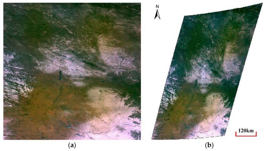
ISPRS Int. J. Geo-Inf. 2021, 10, 406                                                                                               2 of 15

                                       Table 1. Information of the latest geosynchronous satellites.

                                                            Latest                        Spatial        Country or
                                           Series                            Sensor                                     Launch Year
                                                           Satellite                    Resolution/m    Organization
                                         Meteosat       Meteosat-11          SEVIRI          500       European Union       2015
                                         Himawari       Himawari-9            AHI           1000           Japan            2016
                                          INSAT         INSAT-3DR           IMAGER          1000            India           2016
                                          GEOS           GEOS-17              ABI           1000          America           2018
                                          COMS          Cheollian 2B         GOCI-2          250        South Korea         2020

                                             The GF-4 satellite was successfully launched at the Xichang Satellite Launch Center,
                                       China on 29 December 2015. It is the first geosynchronous orbit satellite in China and is
                                       equipped with a starring area array Complementary Metal Oxide Semiconductor (CMOS)
                                       camera that exceeds a 400 km wide swath. The camera can provide a 50 m visible and near
                                       infrared image and a 400 m mid-infrared image; moreover, the former has five bands in
                                       panchromatic, blue, green, red, and near-infrared wavelength [4–6]. The spectral bands are
                                       optional in satellite tasks. Table 2 shows the parameters of the image. The design life of the
                                       GF-4 is 8 years, and the satellite has been safely and stably operated by the China Center
                                       for Resources Satellite Data and Application (CRESDA) for more than 5 years. The daily
                                       schedule is coded into digital instructions and sent ahead to the satellite by 1 to 2 days. In
                                       case of a natural disaster or emergency, the instructions can also be temporarily altered
                                       in a few minutes. Data are freely available to the public, and the relevant information is
                                       accessible at http://36.112.130.153:7777/DSSPlatform/productSearch.html (accessed on
                                       20 March 2021), with the interface in Chinese.

                                                    Table 2. Parameters of the GF-4 image.

                                                                        Spectral         Spatial        Quantity
    Satellite                 Image                 Band                                                                Width/km
                                                                       Range/µm       Resolution/m      Level/bits
                                                    PAN                0.45–0.90
                                                      B1               0.45–0.52
                      Panchromatic and
                                                      B2               0.52–0.60           50              10
      GF-4            Multispectral (PMS)                                                                                  400
                                                      B3               0.63–0.69
                                                      B4               0.76–0.90
                       Mid-infrared (IR)              B5                3.5–4.1           400              12

                                            The ground sample distance (GSD) is the first consideration in practice because it
                                       determines whether or not the targets can be identified in the image. Ground control
                                       points are essential when high geo-positioning accuracy images are required [6,7]. To
                                       examine the quantitative retrieval, radiometric and atmospheric corrections should be
                                       performed with calibration coefficients [8,9]. These coefficients can also be obtained from
                                       the CRESDA website. However, for a satellite with large-area capability such as the GF-
                                       4, the GSD varies considerably in different geolocations. Meanwhile, directly using the
                                       GSD is convenient if the geometric accuracy of the original image sufficiently matches the
                                       application requirements. The calibration coefficients of the previous year can also be used
                                       before those of the later year are released to the public if the radiometric response is stable.
                                       Hence, the stability and reliability of GF-4 images are of great importance for applications,
                                       a feature which is also the most concerning aspect for users.
                                            Several studies have been conducted from one perspective to another [4,10–13].
                                       Wang et al. analyzed the source of GF-4 geometric error and summarized the rule of
                                       error variation. The average external geometric accuracy was improved from 1750 m
                                       to 25 m, and the average internal geometric accuracy was improved from 3.5 pixels to
                                       0.4 pixels after geometric correction [4]. Wei et al. evaluated nine GF-4 images according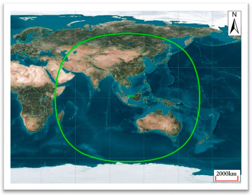
ISPRS Int. J. Geo-Inf. 2021, 10, 406                                                                                              3 of 15

                                       to 630 GCPs in coastal zones and offshore areas and obtained a geolocation uncertainty of
                                       1925 ± 976 m [10]. Li et al. proposed a framework to refine RPC parameters, decreasing
                                       the RMSE of the georeferencing from 3894.4 m to 86.7 m. These studies concentrated on
                                       the geometric quality of GF-4 images, while radiometric quality was rarely discussed in
                                       published literature. The commonly used method is to cross-calibrate the radiometric value
                                       of GF-4 images with a well-calibrated satellite as the reference sensor [13]. However, the
                                       image quality of the GF-4 satellite could vary because of the on-orbit life phases [14–17].
                                       That quality can also be affected by different factors, including the modification of camera
                                       parameters and the motion and jitter of the platform. The evaluation results even vary with
                                       the data acquired on the same day [5,18]. The individual image quality cannot represent
                                       the images in the entire on-orbit lifetime. Therefore, long-term image quality is essential
                                       for users to make better use of the data. For this reason, this article aims to evaluate the
                                       GSD variation with geolocations according to theoretical calculation, and summarize the
                                       geometric and radiometric characteristics over the past 5 years from an analysis of a large
                                       volume of data acquired from the launch.

                                       2. Evaluation of the GSD
                                            The GSD is equivalent to the spatial resolution of an image most of the time. It is also
                                       consistent unless the satellite altitude is greatly adjusted. For example, the GSD decreases
                                       with increasing altitude, and vice versa. For the spatial resolution, all pixels in an image
                                       should be the same after orthorectification. The spatial resolution of the GF-4 released to the
                                       public is 50 m in the visible and near infrared wavelengths and 400 m in the mid-infrared
                                       wavelength. That resolution is only correct for the image acquired at the nadir point or the
                                       neighboring areas. Figure 1 shows the nadir point located at the longitude of 105.6 on the
                                       equator and the scope areas it can capture.

                                       Figure 1. Area scopes that the GF-4 satellite can capture.

                                             The GSD is determined by the instant field of view (IFOV) of the detector, the Earth
                                       curvature, and the satellite altitude. Figure 2a is the schematic diagram of the GSD at
                                       the nadir point. S is the position of the satellite, N is the nadir point, R and L are the
                                       edges of the ground track of a detector, and O is the center of the Earth. According to the
                                       principles of the triangle function, the geocentric angle corresponding to the half of GSD
                                       can be calculated as
                                                                                  (Re + H ) sin θ
                                                                       β = arcsin                 −θ                                 (1)
                                                                                        Re
                                       where β is the geocentric angle, Re is the radius of the Earth, H is the satellite altitude, and
                                       θ is the half IFOV of a detector.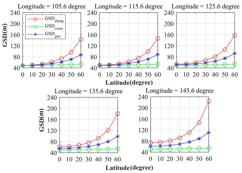
ISPRS Int. J. Geo-Inf. 2021, 10, 406                                                                                                   4 of 15

                                            Then, the GSD can be calculated with a geocentric angle as

                                                                                         (Re + H ) sin θ
                                                         GSDnadi r = 2Reβ = 2Re arcsin                   −θ                               (2)
                                                                                               Re

                                       Figure 2. The schematic diagram of the GSD. (a) the nadir point; (b) off the nadir point.

                                            According to Formula (2) and the designed IFOV value, the GSD is 48.62 m at the
                                       nadir point, an outcome which is better than the released spatial resolution.
                                            The GSD along the imaging direction (hereafter referred to as the along-track direction)
                                       equals that across the imaging direction (hereafter referred to as the across-track direction)
                                       at the nadir point, whereas they are inconsistent at other locations. Figure 2b shows the
                                       schematic diagram of the GSD in the along-track direction at the off-nadir point. The
                                       corresponding GSD can be calculated as

                                                                            GSDal ong = Re( β01 + β02 )
                                                                                                                                          (3)
                                                             = Re(arcsin (Re+ H )Resin(θ +α) + arcsin (Re+ H )Resin(θ −α) − 2θ )

                                       where
                                               (
                                                                                          (Re+ H ) sin(θ +α)          (Re+ H ) sin α
                                                   β01 = ∠ R0 ON − ∠ N 0 ON = arcsin        Re          − arcsin      Re        −θ
                                                     0       0        0              (Re+ H ) sin(θ −α)          (Re+ H ) sin α           (4)
                                                   β 2 = ∠ N ON + ∠ L ON = arcsin           Re          + arcsin     Re         −θ

                                       for which α is the viewing angle of the satellite.
                                            The GSD across the imaging direction is much simpler and can be calculated as

                                                                                            (Re + H 0 ) sin θ

                                                                GSDacr   oss   = 2Re arcsin                   −θ                          (5)
                                                                                                 Re

                                       where
                                                                                     sin β0
                                                                                   H 0 = Re                                  (6)
                                                                                     sin α
                                            In the two-dimensional orthorectified image, the resolutions of the sample and line
                                       in a pixel should be the same. To represent the resolution of a pixel, a geometric GSD is
                                       needed and is represented as
                                                                                   q
                                                                      GSDgeo =         GSDalong × GSDacross                               (7)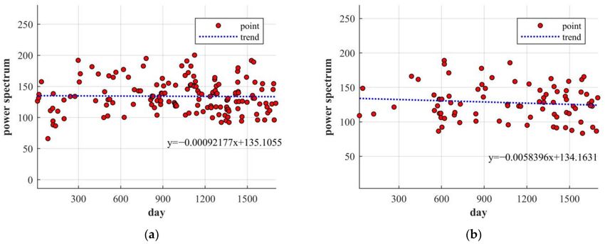
ISPRS Int. J. Geo-Inf. 2021, 10, 406                                                                                          5 of 15

                                            Figure 3 shows the variation of the GSD with the latitude starting from the equator,
                                       and with several longitudes as examples with an interval of 10 degrees. If the interval is
                                       –10 degrees or if latitudes are taken as examples to show the variation of the GSD with
                                       the longitude, the result is the same due to the symmetry of the sphere. The latitude and
                                       longitude ranges do not correspond to the limits that the GF-4 can capture, but the image
                                       distortion beyond the scope is enhanced. Thus, this work shows only the latitude from 0 to
                                       60 and the longitude from 0 to 40 off the nadir point.

                                          Figure 3. The variation of GSD with latitude and longitude.

                                             The GSD in the along-track and across-track directions notably differ. As the distance
                                       increases from the nadir, the GSD in the across-track direction varies little, compared with
                                       that in the along-track direction. When the latitude and longitude are 60 and 40 degrees off
                                       the nadir point, respectively, the variation in the across-track direction is only 1.12 times
                                       that of the nadir point, while it is more than 4.6 times in the along-track direction. The
                                       GSD variance in the longitude of 105.6 reveals the characteristics in one dimension. At the
                                       nadir point, GSDs in the along-track direction and the across-track direction are consistent,
                                       but the gap becomes gradually larger with the increase in latitude. At other points with a
                                       different longitude, GSDs in the along-track direction and the across-track direction are
                                       different even on the equator.
                                             The variation of the GSD also leads to the change of swath and coverage, which are
                                       smallest at the nadir point and largest near the limit of GF-4 capturing capability. This
                                       change is not completely proportional to the GSD due to its difference among pixels in
                                       the same image. Regarding the four corners of the image, the resample size of a corner far
                                       away from the nadir point is much larger than that near the nadir point, thereby causing
                                       the shape of the image to be a distorted diamond. Figure 4 shows the shape of the original
                                       Level 1A image and its orthorectification image in the northeast of China.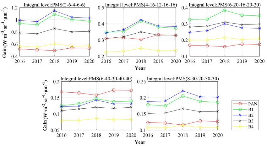
ISPRS Int. J. Geo-Inf. 2021, 10, 406                                                                                                 6 of 15

            Figure 4. Shape of the original Level 1A image (a) and its orthorectification image (b) in the northeast of China.

                                       3. Evaluation of the Geometric Quality of the Image
                                            Geometric quality can be divided into external and internal geometric accuracies.
                                       External geometric accuracy refers to the deviation between the coordinate positions
                                       of checkpoints and their actual positions, also known as absolute positioning accuracy.
                                       Internal geometric accuracy pertains to the deformation of an image which can be regarded
                                       as the consistency among pixels of the entire image or the relative positioning accuracy.

                                       3.1. External Geometric Accuracy
                                            External geometric accuracy is evaluated with level-1A data, and two additional data
                                       are needed. One is Digital Elevation Model (DEM) data extracted from STRM data [19],
                                       released by the U.S. Geological Survey (USGS), and with a spatial resolution of 30 m. The
                                       resolution is comparable with that of GF-4 data. The other is accurate geo-positioning
                                       reference data. Landsat is used here, with a positioning accuracy exceeding 15 m [20]. This
                                       value is precise enough to test the external geometric accuracy of GF-4 data because the
                                       root mean square error (RMSE) of the design requirement is 4 km.
                                            The data selection principle involves covering extensive areas under different terrain
                                       conditions and at least one scene per week to form a long-term dataset. As data before May
                                       2016 are under the commissioning phase, they are restrictively released to the public and
                                       are thus excluded from this work. The data should be of normal quality and cloud-free so
                                       as to facilitate checkpoint selection. The test processes of each scene are as follows:
                                            (1) A total of 20–30 checkpoints that were evenly distributed in the image were selected.
                                       Given the maturity of current image registration technology, this step can be done with
                                       auto-registration software.
                                            (2) Coordinate inverse calculation was conducted with reference data, RPC file, and
                                       DEM data to convert the positions of checkpoints in the reference image from the ground
                                       space to the image space, as represented by the sample and line.
                                            (3) The differences of the samples and lines between the reference image and the
                                       corresponding GF-4 image were calculated as
                                                                                 j     j     j
                                                                               Xi = x i − x i 0
                                                                                 j   j     j                                            (8)
                                                                               Yi = yi − yi 0

                                               j       j
                                       where Xi and Yi are the sample and line errors of the ith checkpoint in scene j, respectively;
                                        j      j                                                                                 j        j
                                       xi and yi are the sample and line of the ith checkpoint in scene j, respectively; xi 0 and yi 0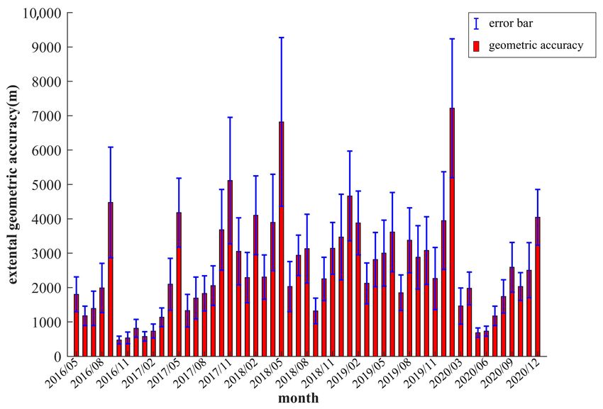
ISPRS Int. J. Geo-Inf. 2021, 10, 406 7 of 15
are the corresponding sample and line of the ith checkpoint converted from the ground
space to the image space.
(4) The mean error was calculated as the external geometric accuracy of the scene as
j n j j
1
µx = n ∑ ( xi − xi 0 )
i =1
j n j j
µy = n1 ∑ (yi − yi 0 ) (9)
ri=1
j 2
2
j
µi = µ x + µy
j j
where µ x and µy are the mean sample and line error of the scene j, respectively, and µi is
the external geometric accuracy of the scene j. The mean sample and line error represent
the errors in the along-track and across-track directions, respectively.
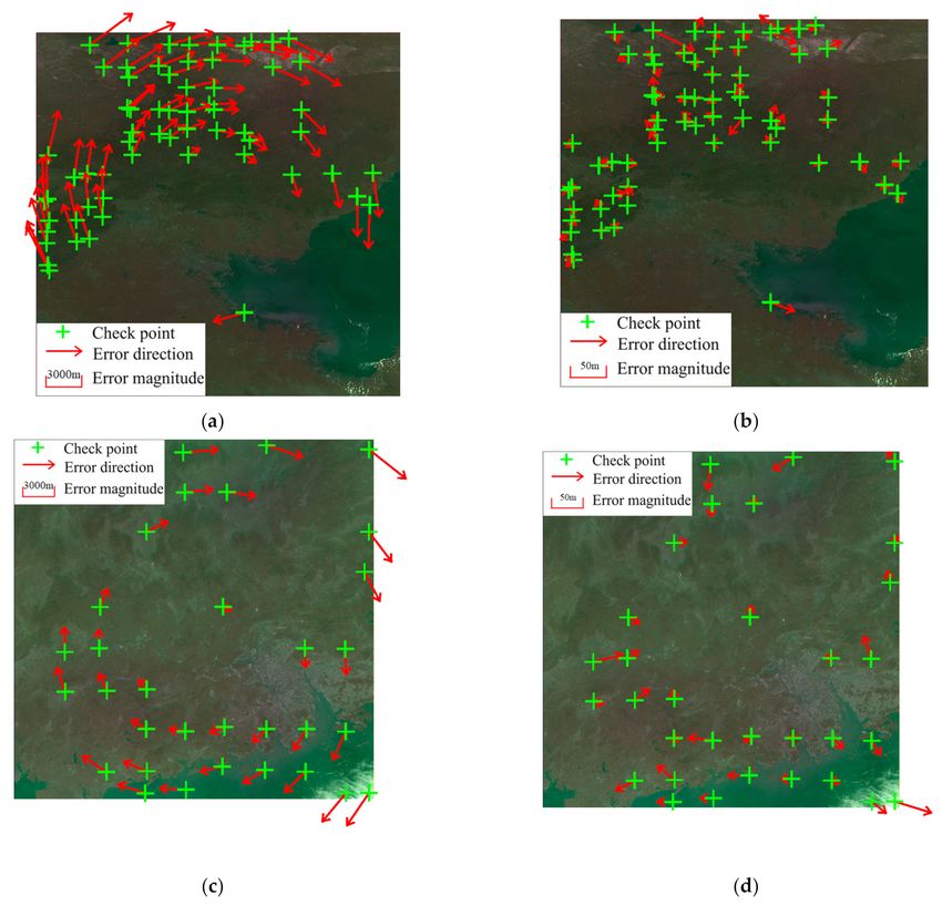
Figure 5 shows the error direction of each scene. From the directionality of the external
geometric accuracy, errors are distributed randomly in four quadrants during the on-orbit
phase, and the average error is approximately zero in either the along-track or cross-track
directions. Thus, no systematic error occurs, otherwise the values would be biased in
a certain direction. The RMSE indicates that 68.3% of the data should meet the design
requirement according to the probability distribution. The external geometric accuracy
is in accord with the expectation as the RMSE is 3.89 km. At the same time, CE90 is also
given as 5.67 km. Given that a few individual outliers were omitted in this study, a low
probability exists that the conclusion may not apply to all data. Although the external
geometric accuracy matches the design requirement, note that not all images have the same
geometric accuracy.
Figure 5. External geometric accuracies of selected GF-4 images.
The average external geometric accuracy of each month represents the absolute posi-
tioning accuracy variance with time (Figure 6). The trend of average external geometric
accuracy gradually increased at certain times, suddenly decreased at some points, and then
increased as usual. This situation arises because the quality control group detected the
deviation of external geometric accuracy when it started to exceed the limit and updated
the parameters of the rigorous geometric model in the ground data processing system so
as to improve the data quality. At the same time, the trend is not completely linear and
occasionally has some randomness, an occurrence which is related to the motion, jitter, and
measurement accuracy of the platform.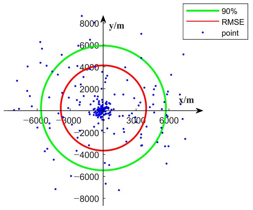
ISPRS Int. J. Geo-Inf. 2021, 10, 406                                                                                            8 of 15

                                       Figure 6. Variation of the external geometric accuracy with time.

                                       3.2. Internal Geometric Accuracy
                                            Internal geometric accuracy generally draws less attention than its external coun-
                                       terpart because its value is so small that it can be ignored. For the push broom image
                                       of a linear array camera, the internal geometric accuracy is considered as the RMSE of
                                       the residuals of checkpoints after removing the external geometric accuracy. However,
                                       for an area array imaging camera such as the GF-4, images are mainly acquired through
                                       the rotation of the satellite. Therefore, in addition to the external geometric accuracy, the
                                       rotation error should also be removed because it can be corrected by altering the rigorous
                                       geometric model. These two errors can be regarded as system errors. After removing them,
                                       the RMSE of residuals reflects the internal geometric accuracy.
                                            Internal geometric accuracy was measured and adjusted in the laboratory before the
                                       launch. The influence of temperature variance from the ground to space means that the
                                       shape of the detector may change slightly, thereby resulting in image distortion. If the
                                       internal geometric accuracy is less than 1 pixel, then the data application will be unaffected.
                                       As the space environment in space is much more stable than that on the ground, the
                                       variation would be minimal in the later phase if the distortion occurs in the early phase
                                       after the launch and was adjusted in the data processing flow. Therefore, only two images
                                       were selected for evaluation in this study. The date of one scene is shortly after the launch,
                                       and that of the other is at the end of December 2020. Figure 7 shows that the relative
                                       errors and direction of the checkpoints in the two images before and after the removal
                                       of system errors. Note that the length of the arrows serves only to enhance the visual
                                       effect and demonstrates the relative value of errors in an image and not the absolute value.
                                       Thus, no comparability occurs between images before and after the removal of external
                                       geometric accuracy.
                                            The errors are directional before systematic correction and randomly distributed after
                                       correction. At the same time, the absolute values of the internal geometric accuracy in
                                       the early phase are 0.67 and 0.57 pixels in the along-track and across-track directions,
                                       respectively, and that of the latest image are 0.54 and 0.65 pixels. All these values meet the
                                       requirement of less than 1 pixel.
ISPRS Int. J. Geo-Inf. 2021, 10, 406 9 of 15
Figure 7. The relative errors and their directions of checkpoints. Errors of an image (a) on 28 August 2016 before removing the
external geometric accuracy; (b) on 28 August 2016 after removing the external geometric accuracy; (c) on 21 December 2020
before removing the external geometric accuracy; (d) on 21 December 2020 after removing the external geometric accuracy.
4. Evaluation of the Radiometric Quality of an Image
Radiometric quality is satisfactory when it performs well in relation to image sharp-
ness and radiometric response. The modulation transfer function (MTF) and signal-noise
ratio (SNR) are commonly used to evaluate image radiometric quality [21,22], especially for
high-resolution images such as IKONOS or QuickBird. However, obtaining a large number
of data containing “knife-edge” targets or uniform areas is difficult because of the compar-
atively low resolution of GF-4 data. Therefore, a power spectrum is instead employed to
evaluate image sharpness and reflects the displacement of the focal plane [23]. Radiometric
calibration was conducted in the laboratory before the launch. Given the long transfer
length along the atmosphere and some other factors, the calibration coefficients should vary
from those obtained in the laboratory. The calibration team of CRESDA routinely updates
and releases the coefficients to the public after conducting annual on-site experiments.
4.1. Image Sharpness
The power spectrum transforms an image from the spatial to the frequency domain so
as to evaluate whether the focal plane of the optical system is displaced or not. The power
spectrum of an image is defined as:
| F (u, v)|2 = F (u, v) ∗ F ∗ (u, v) (10)ISPRS Int. J. Geo-Inf. 2021, 10, 406 10 of 15
where F(u,v) is the Fourier transform of image f(x,y), F ∗ (u, v) is the conjugate function of
F(u,v), u is the horizontal frequency, and v is the vertical frequency.
The power spectrums of two-dimensional images as calculated by the above formula
are not readily comparable to one another. Therefore, to show the trend of the power
spectrum, Formula (11) is typically used to convert a two-dimensional power spectrum
into a one-dimensional counterpart.
◦
1 θ =+180
nρ ∑ ◦
P(ρ) = | F (ρ, θ )|2 (11)
θ =−180
where F (ρ, θ) is the polar formulation of F (u,v), ρ is a radius, θ is an angle, and nρ is the
number of points on the ring with the radius of ρ.
To remove the effect of image size, the power spectrum can be transformed as
◦
θ =+180
1
Mρ × Nρ ∑ ◦
P(ρ) = | F (ρ, θ )|2 (12)
θ =−180
where Mρ is the samples of the image and Nρ is the lines of the image.
To compare a series of images, a variable is used to represent the power spectrum and
is defined as
Z0.5
I= P(ρ)dρ (13)
ρ =0
The image consisting of various land covers is more likely to be detected out of
focus, so images of cities and their neighboring areas are optimal for study. To ensure
the reliability of the evaluation, a long-term time series of images covering Chifeng and
Zhengzhou (which are located in the north and middle of China, respectively) are selected
as contrast experiments. The two cities have high acquired ratios of cloud-free images
which can provide more data for the evaluation. A total of 208 scenes (82 in Zhengzhou
and 157 in Chifeng) from May 2016 to July 2020 were available after strict selection and
filtration.
The scatter plot of the power spectrum and the day shows that simply comparing
the power spectrums of two images fails to truly reflect the change of image sharpness,
as shown in Figure 8. The focus of the optical system always slowly displaces after the
commissioning phase and should not have a sharp change in a short period according
to engineering experience. The imaging time of these images notably vary from the
morning to the afternoon. Hence, the difference between two images is caused not only
by defocusing, but also by the atmosphere condition, season variation, and acquisition
time. The mixed factors complicate the comparison of any two images, but we can also
find some characteristics from the statistical analysis of extensive data. First, the variances
of the power spectrums of the two study areas almost locate in the same value range (a
minimum above 50 and a maximum of approximately 200) and almost no abnormal value
occurs. From this viewpoint, the change of image sharpness is very stable. The average
power spectrum is also concentrated at around 135. Second, the trend analysis shows that
the power spectrums of the two study areas almost coincide. The intercepts of Chifeng and
Zhengzhou are 135.11 and 134.16, respectively, and the slope is negative around zero. If the
statistic scale of the slope is prolonged to a year, then the value is less than 0.1% annually.
This outcome indicates that the image sharpness degrades slightly because of defocusing
and that the degree is low or even negligible. Note that some minor differences arise in the
trend analysis of the slopes and intercepts between Chifeng and Zhengzhou. The main
reason for this result is that the amount of cloud-free data is insufficient. The amount of
data in Zhengzhou in the early years is quite limited. In theory, if a large volume of data is
accumulated in the upcoming years, then the gap should be minimal.ISPRS Int. J. Geo-Inf. 2021, 10, 406 11 of 15
Figure 8. Trend of the power spectrum with time in Chifeng (a) and Zhenzhou (b).
4.2. Radiometric Response
To monitor radiometric response characteristics, ground-based observation experiments
are conducted annually at the Dunhuang test site. The site (40◦ 50 32.8000 N, 94◦ 230 35.7800 E)
is located on the eastern edge of the Kumutage Penniform Desert (which is part of the
Gobi Desert in the northwestern area of China) and lies approximately 35 km to the west of
Dunhuang City, Gansu Province. The land surface covered by cemented gravels is optimal
for the radiometric experiments of satellite sensors [24,25].
The reflectance-based method synchronously measures the surface reflectance, atmo-
spheric data, and other parameters within 30 minutes before and after the flight over the
test site [26]. Ground reflectance is measured with a spectroradiometer device transported
across the entire site. The radiance of a certain band at the sensor is calculated by the 6S
radiative transfer model [27], the input with spectral response function, the solar and satel-
lite angle, and the atmospheric data collected at the same time as the ground reflectance
measurements. The calibration coefficient is then calculated according to the grey level of
image and radiance as
Ra − B
G= (14)
DN
where G is the gain of the radiometric response, B is the bias of the radiometric response, and
both are called calibration coefficients. Ra is the radiance of a certain band at the sensor, and
DN is the corresponding grey level of an image. B is assumed to be stable over these years
and set to be zero in the released version. Given the difference in the integral level settings
of a sensor, the ground tests and corresponding images should include as many possibilities
as possible. Five commonly used settings are shown in Table 3, including the G of visible
and near-infrared bands, and Figure 9 shows the variation of G during 2016 to 2020.
These details are available on http://www.cresda.com/CN/Downloads/dbcs/index.shtml
(accessed on 20 March 2021).
The annual average relative variation is used to evaluate the stability of the radiometric
response as
− Avei
Vi = Gi Ave × 100%
i
N
∑ Vi
(15)
i =0
V= N
where Vi is the variance of the calibration coefficient in the ith year, Avei is the average
value of the calibration coefficient of G, and V is the annual average relative variation.ISPRS Int. J. Geo-Inf. 2021, 10, 406 12 of 15
Table 3. The calibration coefficients of each band with different integral parameters from 2016 to 2020.
Integral Level Band 2016 2017 2018 2019 2020
PAN 0.5215 0.5061 0.4933 0.5395 0.5329
B1 0.94 0.9175 1.0904 1.0028 0.9767
PMS (2-6-4-6-6) B2 0.9885 0.9691 1.1484 1.0418 1.0278
B3 0.7847 0.7715 0.8558 0.8017 0.809
B4 0.5641 0.5512 0.6046 0.5655 0.5738
PAN 0.31 0.3151 0.3043 0.3327 0.3293
B1 0.3484 0.3511 0.4175 0.3803 0.3728
PMS (4-16-12-16-16) B2 0.3448 0.3641 0.4244 0.3863 0.3833
B3 0.3095 0.3207 0.3505 0.3299 0.331
B4 0.2257 0.2314 0.2494 0.2343 0.2363
PAN 0.1683 0.1647 0.159 0.1752 0.1733
B1 0.3263 0.3286 0.3833 0.3531 0.349
PMS (6-20-16-20-20) B2 0.2472 0.2578 0.2998 0.275 0.2719
B3 0.2806 0.2858 0.3109 0.2946 0.2988
B4 0.1997 0.1999 0.215 0.2038 0.2082
PAN 0.1678 0.1647 0.1577 0.1735 0.1725
B1 0.1252 0.1315 0.1468 0.1375 0.1395
PMS (6-40-30-40-40) B2 0.1226 0.1239 0.1427 0.1308 0.1312
B3 0.1102 0.1154 0.1205 0.1171 0.1203
B4 0.0796 0.0802 0.0858 0.0818 0.083
PAN 0.1235 0.1221 0.116 0.1288 0.1266
B1 0.1784 0.1749 0.2053 0.1887 0.1858
PMS (8-30-20-30-30) B2 0.1878 0.1903 0.2209 0.203 0.2013
B3 0.1515 0.1532 0.1664 0.1569 0.158
B4 0.108 0.1073 0.115 0.1084 0.1087
The integral level parameter is represented in the order of wavelength band PAN, B1,
B2, B3 and B4 (PAN-B1-B2-B3-B4). The most stable performance occurs under the integral
level parameter (8-30-20-30-30). The annual average relative variation has the lowest value
at 3.29%, and the corresponding values of panchromatic, B1, B2, B3, and B4 are 2.82%,
4.45%, 4.63%, 2.54% and 2.02%, respectively. The maximum value with the parameter
(4-16-12-16-16) is 3.95%, and the corresponding values of each band are 3.20%, 5.32%, 5.49%,
3.22% and 2.52%. The stability of each band also varies with different integration level
parameters. B4 seems to be the most stable band, for which the average annual relative
variation is less than 3%, followed by B3 and the panchromatic band. The uncertainty in the
experiment process is greater than the variance among different integral level parameters
or bands, and the maximum variance is only 5.5%. Thus, the changing rate is acceptable.
Many uncertainty factors can affect the accuracy, such as the operating specificity of the
spectroradiometer, the non-Lambertian characteristics, the uniformity of the test site, and
the change of the solar zenith angle during the measurement.ISPRS Int. J. Geo-Inf. 2021, 10, 406 13 of 15
Figure 9. The calibration coefficients from 2016 to 2020.
5. Discussion
In general, the image quality evaluation of a remote sensing satellite includes geo-
metric and radiometric quality [28]. Evaluation methods are common when it comes to
geometric quality, i.e., comparing the target image with high-precision reference map by
image registration technology. The external geometric accuracy of well-known geosyn-
chronous orbit satellites such as GEOS-8, Meteosat-1 and INSAT-3D are measured by the
above methods, and the accuracies are 4 to 6 km [29], 4 to 5 km [30] and 10 to 20 km [28],
respectively. From the results in this paper, the geometric accuracy of GF-4 images is
comparable with those of most geosynchronous orbit satellites, which shows the reliability
of the method and the results. Surprisingly, the geometric accuracy of Himawari-8 image
is close to 1 pixel. Note that the data are supposed to be geometrically corrected and then
released to the public. Radiometric evaluation methods also vary with different satellites.
The commonly used technique is SNR and MTF, especially for high-resolution images.
Given the comparatively low resolution of GF-4 images, data containing “knife-edge”
targets or uniform areas are difficult to obtain. Therefore, SNR and MTF are not used and
power spectrum is instead employed to evaluate image sharpness. The results reflect the
stability of the image sharpness and show no displacement of the focal plane. Moreover,
radiometric response is a key factor of image quality. The radiometric coefficients of most
satellites such as Landsat, Terra MODIS and EO-1 Hyperion [31,32] have been monitored
for many years, which shows that this method is well recognized. The cameras have
degraded in radiometric response by 10% since the launch of the EOS/Terra spacecraft [32],
and the degradation rate is greater than that of GF-4. GSD is also a frequently applied
image quality index for most satellites, and it varies considerably with geolocations [22].
Thus, the analysis of the GSD variation is useful for users before they consider GF-4 images
as an application data source. Given that the Earth’s curvature and satellite altitude are
constant, and we can deduce the IFOV according to the GSD at the nadir point, so the image
GSD variation with geolocations is evaluated by theoretical value instead of measuring it
in the image, which can also avoid the measuring errors in the actual images.
6. Conclusions
In this study, the evaluation of the quality of GF-4 satellite images is conducted from
three aspects: GSD, geometric quality, and radiometric quality. Theoretical description and
data analysis reveal the following conclusions.
The spatial resolution released to the public with 50 m in panchromatic and multi-
spectral bands and 400 m in mid-infrared is only true under the condition that the imageISPRS Int. J. Geo-Inf. 2021, 10, 406 14 of 15
is acquired at nadir point or at the neighboring areas. For other regions of interest, the
GSD increases gradually with the distance away from the nadir point. If the orthorectifica-
tion is implemented with the level 1A image, the spatial resolution parameters should be
determined by the longitude and latitude.
The geometric quality is evaluated from the external and internal geometric accura-
cies. The external geometric accuracy error directions evaluated on extensive images are
inconsistent, so the judgment can be made that no systematic error occurs. Most of the
errors are also within the design requirements of 4 km. The internal geometric accuracy
can be evaluated from the RMSE of the residual errors of the checkpoints after removing
the systematic errors. The images acquired in the early and latest phases show that the
accuracy is less than 1 pixel and meets the design requirements.
The radiometric quality of GF-4 images is evaluated in terms of image sharpness
and radiometric response. The long-term monitoring results reveal that the variances
of the power spectrum locate in a certain value range and indicates that the change of
image sharpness is stable. However, the absolute value of one scene may differ from
another because of the inconsistent imaging time and season or other affecting factors. The
radiometric response is evaluated by the radiometric calibration coefficients according to
annual on-site experiments. Moreover, the radiometric response of different bands and
integral level parameters perform well with little degradation.
Author Contributions: Conceptualization, writing—review and editing, supervision, project admin-
istration, Wei Yi and Yuhao Wang; methodology, validation, formal analysis, Yong Zeng; investigation,
data curation, visualization, Yaqing Wang; writing—original draft preparation, Jianfei Xu. All authors
have read and agreed to the published version of the manuscript.
Funding: This work was funded by the Qianxuesen Innovation Foundation of China Aerospace
Science and Technology Corporation (2020) and the National Natural Science Foundation of China
(71771024).
Institutional Review Board Statement: Ethical review and approval were waived for this study, due
to the data being sourced from an open platform.
Informed Consent Statement: Not applicable.
Data Availability Statement: Publicly available datasets were analyzed in this study. This data can
be found here: (1) images were provided by official website of China Center for Resources Satellite
Data and Application: http://36.112.130.153:7777/DSSPlatform/productSearch.html (accessed on
20 March 2021). (2) The calibration coefficients were also provided by official website of China Center
for Resources Satellite Data and Application: http://www.cresda.com/CN/Downloads/dbcs/index.
shtml (accessed on 20 March 2021).
Acknowledgments: The authors would like to thank the reviewers for their professional opinions
and the hard work of the editorial department, which greatly promoted the improvement of the
quality of the article. The authors would like to thank China Center for Resources Satellite Data and
Application for providing us with data support.
Conflicts of Interest: The authors declare no conflict of interest.
References
1. He, Y.; Xu, M.; Jia, X.; Armellin, R. High-precision repeat-groundtrack orbit design and maintenance for Earth observation
missions. Celest. Mech. Dyn. Astron. 2017, 128, 275–294. [CrossRef]
2. Saboori, B.; Bidgoli, A.M.; Saboori, B. Multiobjective Optimization in Repeating Sun-Synchronous Orbits Design for Remote-
Sensing Satellites. J. Aerosp. Eng. 2014, 27, 04014027. [CrossRef]
3. Li, D.; Wang, M.; Jiang, J. China’s high-resolution optical remote sensing satellites and their mapping applications. Geo-Spat. Inf.
Sci. 2020. [CrossRef]
4. Wang, M.; Cheng, Y.; Chang, X.; Jin, S.; Zhu, Y. On-orbit geometric calibration and geometric quality assessment for the
high-resolution geostationary optical satellite GaoFen4. ISPRS J. Photogramm. Remote Sens. 2017, 125, 63–77. [CrossRef]
5. Wang, M.; Cheng, Y.; Tian, Y.; He, L.; Wang, Y. A New On-Orbit Geometric Self-Calibration Approach for the High-Resolution
Geostationary Optical Satellite GaoFen4. IEEE J. Sel. Top. Appl. Earth Obs. Remote Sens. 2018, 11, 1670–1683. [CrossRef]ISPRS Int. J. Geo-Inf. 2021, 10, 406 15 of 15
6. Yang, B.; Pi, Y.; Li, X.; Wang, M. Relative Geometric Refinement of Patch Images Without Use of Ground Control Points for the
Geostationary Optical Satellite GaoFen4. IEEE Trans. Geosci. Remote Sens. 2018, 56, 474–484. [CrossRef]
7. Toutin, T. Review article: Geometric processing of remote sensing images: Models, algorithms and methods. Int. J. Remote Sens.
2004, 25, 1893–1924. [CrossRef]
8. Cai, L.; Bu, J.; Tang, D.; Zhou, M.; Yao, R.; Huang, S. Geosynchronous Satellite GF-4 Observations of Chlorophyll-a Distribution
Details in the Bohai Sea, China. Sensors 2020, 20, 5471. [CrossRef]
9. Chen, Y.; Sun, K.; Li, D.; Bai, T.; Huang, C. Radiometric Cross-Calibration of GF-4 PMS Sensor Based on Assimilation of Landsat-8
OLI Images. Remote Sens. 2017, 9, 811. [CrossRef]
10. Wei, Y.; Zhang, Z.; Mu, B.; Li, Y.; Wang, Q.; Liu, R. Geolocation Accuracy Evaluation of GF-4 Geostationary High-Resolution
Optical Images over Coastal Zones and Offshore Areas. J. Coast. Res. 2020, 102, 326–333. [CrossRef]
11. Han, L.; Gao, K.; Dou, Z.; Zhu, Z.; Wang, H.; Fu, X. On-Orbit MTF Estimation for GF-4 Satellite Using Spatial Multisampling on a
New Target. IEEE Geosci. Remote Sens. Lett. 2020, 17, 17–21. [CrossRef]
12. Li, P.; Sun, K.; Li, D.; Sui, H.; Zhang, Y. An Emergency Georeferencing Framework for GF-4 Imagery Based on GCP Prediction
and Dynamic RPC Refinement. Remote Sens. 2017, 9, 1053. [CrossRef]
13. Yang, A.; Zhong, B.; Wu, S.; Liu, Q. Radiometric Cross-Calibration of GF-4 in Multispectral Bands. Remote Sens. 2017, 9, 232.
[CrossRef]
14. Martin-Neira, M.; Oliva, R.; Corbella, I.; Torres, F.; Duffo, N.; Duran, I.; Kainulainen, J.; Closa, J.; Zurita, A.; Cabot, F.; et al. SMOS
instrument performance and calibration after six years in orbit. Remote Sens. Environ. 2016, 180, 19–39. [CrossRef]
15. Wenny, B.N.; Helder, D.; Hong, J.; Leigh, L.; Thome, K.J.; Reuter, D. Pre- and Post-Launch Spatial Quality of the Landsat 8
Thermal Infrared Sensor. Remote Sens. 2015, 7, 1962–1980. [CrossRef]
16. Schwerdt, M.; Schmidt, K.; Klenk, P.; Ramon, N.T.; Rudolf, D.; Raab, S.; Weidenhaupt, K.; Reimann, J.; Zink, M. Radiometric
Performance of the TerraSAR-X Mission over More Than Ten Years of Operation. Remote Sens. 2018, 10, 754. [CrossRef]
17. Jiang, B.; Liang, S.; Townshend, J.R.; Dodson, Z.M. Assessment of the Radiometric Performance of Chinese HJ-1 Satellite CCD
Instruments. IEEE J. Sel. Top. Appl. Earth Obs. Remote Sens. 2013, 6, 840–850. [CrossRef]
18. Crowley, C.; Kohley, R.; Hambly, N.C.; Davidson, M.; Abreu, A.; van Leeuwen, F.; Fabricius, C.; Seabroke, G.; de Bruijne, J.H.J.;
Short, A.; et al. On-orbit performance of the Gaia CCDs at L2. Astron. Astrophys. 2016, 595, 17. [CrossRef]
19. Reuter, H.I.; Nelson, A.; Jarvis, A. An evaluation of void-filling interpolation methods for SRTM data. Int. J. Geogr. Inf. Sci. 2007,
21, 983–1008. [CrossRef]
20. Gill, T.; Collett, L.; Armston, J.; Eustace, A.; Danaher, T.; Scarth, P.; Flood, N.; Phinn, S. Geometric correction and accuracy
assessment of Landsat-7 ETM+ and Landsat-5 TM imagery used for vegetation cover monitoring in Queensland, Australia from
1988 to 2007. J. Spat. Sci. 2010, 55, 273–287. [CrossRef]
21. Crespi, M.; De Vendictis, L. A Procedure for High Resolution Satellite Imagery Quality Assessment. Sensors 2009, 9, 3289–3313.
[CrossRef] [PubMed]
22. Ryan, R.; Baldridge, B.; Schowengerdt, R.A.; Choi, T.; Helder, D.L.; Blonski, S. IKONOS spatial resolution and image interpretabil-
ity characterization. Remote Sens. Environ. 2003, 88, 37–52. [CrossRef]
23. Tao, S.; Jin, G.; Zhang, X.; Qu, H.; An, Y. Wavelet power spectrum-based autofocusing algorithm for time delayed and integration
charge coupled device space camera. Appl. Opt. 2012, 51, 5216–5223. [CrossRef] [PubMed]
24. Zhang, H.; Zhang, B.; Chen, Z.; Huang, Z. Vicarious Radiometric Calibration of the Hyperspectral Imaging Microsatellites
SPARK-01 and-02 over Dunhuang, China. Remote Sens. 2018, 10, 120. [CrossRef]
25. Gao, C.; Zhao, Y.; Li, C.; Ma, L.; Wang, N.; Qian, Y.; Ren, L. An Investigation of a Novel Cross-Calibration Method of FY-3C/VIRR
against NPP/VIIRS in the Dunhuang Test Site. Remote Sens. 2016, 8, 77. [CrossRef]
26. Thome, K.J. Absolute radiometric calibration of Landsat 7 ETM+ using the reflectance-based method. Remote Sens. Environ. 2001,
78, 27–38. [CrossRef]
27. Vermote, E.F.; Tanre, D.; Deuze, J.L.; Herman, M.; Morcrette, J.J. Second Simulation of the Satellite Signal in the Solar Spectrum,
6S: An overview. IEEE Trans. Geosci. Remote Sens. 1997, 35, 675–686. [CrossRef]
28. Jindal, D.; Prakash, S.; Sanghvi, J.; Kartikeyan, B.; Krishna, B.G. INSAT-3D Quality Analysis System (i3dQAS). In ISPRS Technical
Commission Viii Symposium; Dadhwal, V.K., Diwakar, P.G., Seshasai, M.V.R., Raju, P.L.N., Hakeem, A., Eds.; ISPRS: Hannover,
Germany, 2014; Volume 40–48, pp. 257–263.
29. Ellrod, G.P.; Achutuni, R.V.; Daniels, J.M.; Prins, E.M.; Nelson, J.P. An assessment of GOES-8 imager data quality. Bull. Am.
Meteorol. Soc. 1998, 79, 2509–2526. [CrossRef]
30. Jones, M.; Colombeski, N.C. Image quality control in the Meteosat Ground Processing System. Int. J. Remote Sens. 1981, 2, 331–349.
[CrossRef]
31. Helder, D.; Thome, K.J.; Mishra, N.; Chander, G.; Xiong, X.; Angal, A.; Choi, T. Absolute Radiometric Calibration of Landsat
Using a Pseudo Invariant Calibration Site. IEEE Trans. Geosci. Remote Sens. 2013, 51, 1360–1369. [CrossRef]
32. Bruegge, C.J.; Val, S.; Diner, D.J.; Jovanovic, V.; Gray, E.; Di Girolamo, L.; Zhao, G. Radiometric stability of the Multi-angle
Imaging SpectroRadiometer (MISR) following 15 years on-orbit. In Earth Observing Systems Xix; Butler, J.J., Xiong, X., Gu, X., Eds.;
International Society for Optics and Photonics: Bellingham, WA, USA, 2014; Volume 9218.You can also read