Computers, Environment and Urban Systems - Infoscience
←
→
Page content transcription
If your browser does not render page correctly, please read the page content below
Computers, Environment and Urban Systems 85 (2021) 101549
Contents lists available at ScienceDirect
Computers, Environment and Urban Systems
journal homepage: www.elsevier.com/locate/ceus
Estimating quality of life dimensions from urban spatial pattern metrics
Marta Sapena a, b, Michael Wurm b, Hannes Taubenböck b, c, Devis Tuia d, e, *, Luis A. Ruiz a
a
Geo-Environmental Cartography and Remote Sensing Group, Department of Cartographic Engineering, Geodesy and Photogrammetry, Universitat Politècnica de
València, Camí de Vera, s/n, 46022 Valencia, Spain
b
German Aerospace Center (DLR), German Remote Sensing Data Center (DFD), Oberpfaffenhofen, 82234 Wessling, Germany
c
Institute for Geography and Geology, Julius-Maximilians-Universität Würzburg, 97074 Würzburg, Germany
d
Laboratory of Geo-Information Science and Remote Sensing, Wageningen University, 6700, PB, Wageningen, the Netherlands
e
Environmental Computational Science and Earth Observation Laboratory, Ecole Polytechnique Fédérale de Lausanne, 1950 Sion, Switzerland
A R T I C L E I N F O A B S T R A C T
Keywords: The spatial structure of urban areas plays a major role in the daily life of dwellers. The current policy framework
Spatial metrics to ensure the quality of life of inhabitants leaving no one behind, leads decision-makers to seek better-informed
Socio-economic variables choices for the sustainable planning of urban areas. Thus, a better understanding between the spatial structure of
Local climate zones
cities and their socio-economic level is of crucial relevance. Accordingly, the purpose of this paper is to quantify
Quality of life
this two-way relationship. Therefore, we measured spatial patterns of 31 cities in North Rhine-Westphalia,
Remote sensing
Germany. We rely on spatial pattern metrics derived from a Local Climate Zone classification obtained by
fusing remote sensing and open GIS data with a machine learning approach. Based upon the data, we quantified
the relationship between spatial pattern metrics and socio-economic variables related to ‘education’, ‘health’,
‘living conditions’, ‘labor’, and ‘transport’ by means of multiple linear regression models, explaining the vari
ability of the socio-economic variables from 43% up to 82%. Additionally, we grouped cities according to their
level of ‘quality of life’ using the socio-economic variables, and found that the spatial pattern of low-dense built-
up types was different among socio-economic groups. The proposed methodology described in this paper is
transferable to other datasets, levels, and regions. This is of great potential, due to the growing availability of
open statistical and satellite data and derived products. Moreover, we discuss the limitations and needed con
siderations when conducting such studies.
1. Introduction Lavalle, 2014; Taubenböck et al., 2012). The quality of life and sustain
able development of urban and peri-urban areas depend on the successful
How we organize space in urban areas has a decisive influence on management of their growth. Both are common goals in cities around
how we live and what effects this has on our closest environment: what the world. They are described in multiple dimensions: ‘quality of life’ is a
kind of mobility we choose, how large our ecological footprint is, how broad concept assessed on various factors ranging from living conditions
close we are to utilities, or what access we have to jobs or leisure fa and employment to experience of life. It is usually represented by a
cilities. These are just a few of the many exemplary factors that influence multiple set of indicators such as income, deprivation rate, education
the quality of life and the sustainability by its spatial design. attainment, employment rate, life expectancy, air quality, etc. (Eurostat,
This is especially relevant in cities, as the world population is 2017; OECD, 2017). Also ‘sustainable development’ is addressed by the
becoming urban. The share of people living in urban areas has been United Nations in their 2030 Agenda for Sustainable Development. It
growing in the last decades and this trend is expected to continue collects seventeen Sustainable Development Goals (SDGs), which aim at
(United Nations, 2018). Heretofore, population growth has been ending poverty by means of promoting economic growth, addressing
accompanied by a significant increase of the urban layout, triggering social needs, while protecting the environment and fighting climate
environmental and socio-economic consequences (e.g. Haase, Kabisch, change.
& Haase, 2013; Ribeiro-Barranco, Batista e Silva, Marin-Herrera, & Urban form is constituted by spatial and socio-economic processes
* Corresponding author at: Laboratory of Geo-Information Science and Remote Sensing, Wageningen University, 6700, PB, Wageningen, the Netherlands.
E-mail addresses: marta.sapena-moll@dlr.de (M. Sapena), michael.wurm@dlr.de (M. Wurm), hannes.taubenboeck@dlr.de (H. Taubenböck), devis.tuia@wur.nl
(D. Tuia), laruiz@cgf.upv.es (L.A. Ruiz).
https://doi.org/10.1016/j.compenvurbsys.2020.101549
Received 9 April 2020; Received in revised form 31 August 2020; Accepted 20 September 2020
0198-9715/© 2020 The Authors. Published by Elsevier Ltd. This is an open access article under the CC BY license (http://creativecommons.org/licenses/by/4.0/).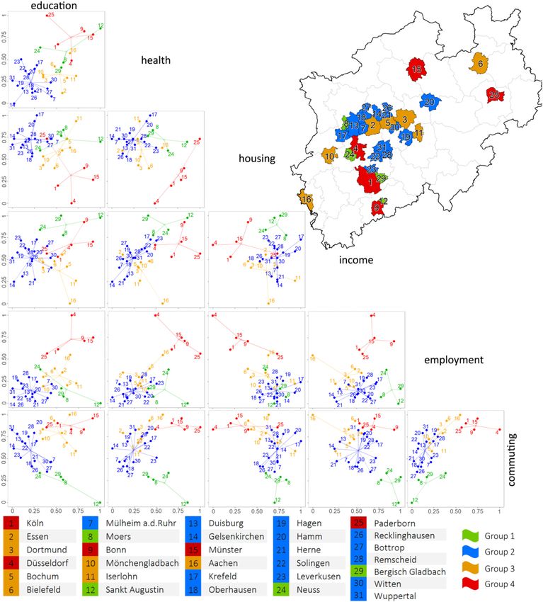
M. Sapena et al. Computers, Environment and Urban Systems 85 (2021) 101549
developed over time and space (Abrantes et al., 2019; Salat, 2011). It is economic databases, studies aiming to quantify the relations between
accepted in scientific literature to wield a powerful influence on shaping the spatial structure of urbanized areas and the quality of life of in
societies (Oliveira, 2016; Salat, 2011; Tonkiss, 2013). Urban form is a habitants or the well-known SDGs are still scarce. Methods based on the
key element for understanding urban systems as it drives where people quantification of spatial patterns by means of spatial metrics and the
live and work and how the interaction is spatially structured (e.g. clustering of urban areas based on their socio-economic performance (e.
Grimm, Cook, Hale, & Iwaniec, 2015; Taubenböck, 2019). However, it is g.: Abrantes et al., 2019; Sapena, Ruiz, & Goerlich, 2016; Schwarz,
not self-evident to establish a universal link between the urban spatial 2010) have shown to be suitable for the combined analysis of spatial and
structure, here considered as the organization of urban areas in terms of socio-economic variables in urban areas as well as for their relation.
the distribution of physical structures and human activities (Krehl & In this framework, the general objective of this work is to understand
Siedentop, 2019), and quality of life. Accordingly, in this study we want better the relationship between the spatial structure of cities and the
to explicitly investigate this relation between urban structural features socio-economic level of city dwellers. For this reason, we explore the
and socio-economic parameters, and whether quality of life can be value of the LCZ, as urban structural types, in relation to quality of life
interpreted based on spatial and statistical methods. indicators at the city level. First, we quantify the relationships between
Urban areas with similar physical appearance tend to feature similar socio-economic variables and the spatial distribution of LCZ. Then, we
social, economic, and environmental characteristics (Patino & Duque, group cities according to their similar levels of quality of life and
2013; Taubenböck et al., 2009; Wurm & Taubenböck, 2018). Conse describe their spatial structure.
quently, several authors have described qualitatively and quantitatively
these influences. Concerning social factors, many relevant concerns such 2. Data
as crime, public safety, gentrification, health, and poverty, have been
linked to diversity and configuration of land uses, road network pat 2.1. Study area
terns, or remote sensing derived variables (e.g. Hankey & Marshall,
2017; Jacobs, 1961; Lehrer & Wieditz, 2009; Patino, Duque, Pardo- We selected North Rhine-Westphalia (NRW) as a study case for its
Pascual, & Ruiz, 2014; Sandborn & Engstrom, 2016; Wurm et al., socio-economic relevance in Europe, reinforced by the availability of
2019). In terms of economic issues, wealth indicators were positively statistical data. The historical and political background of many cities
related to the diversity of land uses, and productivity and innovation located in this Federal State is similar, which diminishes external in
were influenced by density, centricity, and urban size (e.g. Tapiador, fluences in our analysis. We base our study on a sample of 31 cities in
Avelar, Tavares-Corrêa, & Zah, 2011; UN-Habitat, 2015). For the envi NRW as consistent spatial and socio-economic databases are available
ronmental dimension, the identification of land cover and urban struc there. The location and identification of cities is presented below in
tural types allowed for instance determining urban heat islands or green Fig. 2.
area facilities, which contributed to climate change studies (Bechtel Regarding the Federal State of NRW, it is the most populous of the
et al., 2019; Stewart & Oke, 2012), while pollution, energy use, and sixteen German states, accounting for 21.7% of the total population in
transport means have also been related to different properties of urban Germany (Eurostat, 2019). The Ruhr industrial region, in NRW, is a
form, such as density, diversity or centrality of land use (e.g. Anderson, competitive industrial region of Germany. NRW is an economic centre in
Kanaroglou, & Miller, 1996; Hankey & Marshall, 2017). However, there Europe, with a regional GDP of € 672 billion in 2016 (21.4% of the
are few studies that measure this widely agreed linkage between the German GDP). However, the per capita level is slightly below the na
spatial structure of cities and their socio-economic status in a quanti tional level. Nowadays, the economy of NRW is based on small and
tative manner. These studies mostly rely on earth observation data to medium-sized enterprises, hosting more than 20% of companies in
extract the physical information, such as buildings, roads, land-use/ Germany, and providing work to near 80% of the active population
land-cover (LULC) and their spatial distribution, or structure and (European Commission, 2019).
texture features. This approach has been applied so far to model
neighborhood deprivation (Venerandi, Quattrone, & Capra, 2018), 2.2. Socio-economic variables
poverty (Duque, Patino, Ruiz, & Pardo-Pascual, 2015; Jean et al., 2016;
Wurm & Taubenböck, 2018), income and property value (Taubenböck For the socio-economic analysis we used the City statistics database
et al., 2009), and demographic, living conditions, labor and transport (https://ec.europa.eu/eurostat/web/cities/data/database). This data
factors (Sapena, Ruiz, & Goerlich, 2016). These examples present pre base was originally created with the purpose to provide information that
vious attempts to identify links between urban spatial structure and supports more evidence-based decisions in planning and managing tasks
socio-economic parameters. (Eurostat, 2016). The City statistics project covers several aspects of
Insofar, the investigation of these relations has been possible due to quality of life – i.e., demography, housing, health, economic activity,
the increasing accessibility of open databases and earth observation labour market, income disparity, educational qualifications, environ
products. On the one hand, satellite images allow for increasing capa ment, climate, travel patterns, tourism, and cultural infrastructure - for
bilities to provide high-resolution geoinformation. In this context, LULC cities and their commuting zones in Europe (Eurostat, 2018). At the city
data have been an important source of information for urban studies; level, it contains 171 variables and 62 indicators for more than one
however, it lacks three-dimensional information of urban structures, thousand cities that have an urban core of at least 50,000 inhabitants.
considered a fundamental aspect in such studies (Wentz et al., 2018). The data are available at different dates from 1990 onwards. In this
Therefore, the characterization of cities into urban structural types and study the city level is the basic spatial unit. At this level a rich source of
land cover, with Local Climate Zones (LCZ) (Stewart & Oke, 2012) as data for comparative studies in Europe is provided.
one concept, has great potential in its relation with socio-economic For the purpose of this study, we selected a set of socio-economic
functions (Bechtel et al., 2015). LCZ have additional inherent informa variables and indicators for 31 cities in NRW for the year 2009
tion on the physical composition of cities compared to other LULC leg (Table 1), to coincide with the date of the satellite images used for LCZ
ends by their density, building types, heights, greenness and their land classification. When data from 2009 were not available, the previous or
cover that are worth to explore. Besides, it is a conceptually consistent, subsequent year was used instead. Subject to the availability of data, we
generic, and culturally-neutral description and thus a replicable classi selected indicators of five dimensions of ‘quality of life’ covered in the
fication system. On the other hand, global, national and local institutes database – education, health, living condition, labor and transport. We
provide more and more statistical data for different dates and spatial linked the dimensions to the SDGs policy commitments, as was previ
levels. Notwithstanding all the urban theories relating these two com ously done by the OECD (2017) to evidence the global efforts that are
ponents, and the growing availability of both, spatial and socio- being made to reduce inequalities in the socio-economic level of citizens
2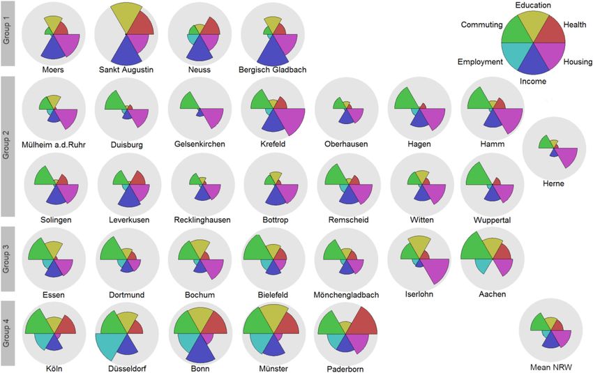
M. Sapena et al. Computers, Environment and Urban Systems 85 (2021) 101549
Table 1
Description of the selected socio-economic variables (dependent variables in the models from Table 5) representing five dimensions of quality of life and their link to
the Sustainable Development Goals (SDGs).
Dimension Name Description SDGs
Education education The proportion of population (aged 25–64) with lower secondary as the highest level of SDG 4 (education)
education
Health health Crude death rate per 1000 inhabitants SDG 3 (health)
Living housing Average price for buying an apartment in euros SDG 1 and 11 (poverty and sustainable cities)
conditions income Median disposable annual household income in euros
affordability Ratio reflecting the ability of a city to pay for housing. Housing price compared to income.
Labor employment Number of employments per 1000 inhabitants (work place-based) SDG 8 (decent work and economy)
Transport transport The share of journeys to work by car or motor cycle (%) SDG 9 and 11 (Infrastructure and sustainable
commuting People commuting out of the city per 1000 residents cities)
(Table 1). extracted for each cell (Table 2) to train the classifier. A ground truth of
2658 cells was defined by photointerpretation, where the cognitive
2.3. Earth observation and ancillary data perception of an interpreter was used to define the predominant LCZ.
The classifier was based on random forests, a method building
For classification of the physical structures describing the cities’ several decision trees with heavy randomization of features (Breiman,
spatial structure we rely on remotely sensed and geospatial data 2001). The initial result was then further improved by making the model
extracted from three data sources: aware of two spatial relationships between cells using a Markovian
Random Field formulation (see Tuia, Moser, Wurm, & Taubenböck
- High-resolution remote sensing imaging: a Rapid-Eye mosaic for the (2017)): (1) By predicting with higher probability co-occurrence of
year 2009 was constructed for the whole area. This satellite provides neighboring LCZ that attract or repel each other spatially; (2) By fa
images at 6.5 m resolution (orthorectified and resampled to 5 m) voring a map respecting a rank-size distribution of urban settlements,
with five spectral bands (red, green, blue, near infrared and red according to Zipf’s law.
edge). For testing the relationships between socio-economic and spatial
- 3D model: A normalized digital surface model (nDSM) was derived structure of cities, we extracted a large set of spatial pattern metrics,
from 135 individual Cartosat-1 stereo images (collected between henceforth referred to as spatial metrics, related to attributes such as
2009 and 2013) and processed according to Wurm, d’Angelo, Rein density, aggregation, shape, etc., using the spatial module of the soft
artz, & Taubenböck (2014) to retrieve above ground heights. ware tool IndiFrag (Sapena & Ruiz, 2015). This tool computes spatio-
- GIS layers from OpenStreetMap: the amenities and road layers from temporal metrics that quantify spatial patterns and their changes from
the open repository of geospatial data was used (downloaded in thematic maps. We used the LCZ classification as a base to characterize
2014, openstreetmap.org). the spatial structure of cities. The level of analysis to extract the spatial
metrics was the city level that corresponds to the level in which the
socio-economic variables are provided. Therefore, we computed all
3. Methods
spatial metrics included in IndiFrag, obtaining one set of metrics per LCZ
class for the spatial level of the city, and another set of metrics for the
3.1. Patterns describing the spatial structure of cities
city, regardless of the LCZ classes. Then, we standardized the values of
For the derivation of the spatial patterns describing the spatial
structure of cities, we applied the LCZ framework that allows charac
terizing the morphologic appearance of cities in a conceptually consis Table 2
Description of the geo-spatial variables for each cell from remote sensing and
tent manner. It comprises several urban structural and land covers types
GIS data.
with uniform surface cover, structure, material and use (Stewart & Oke,
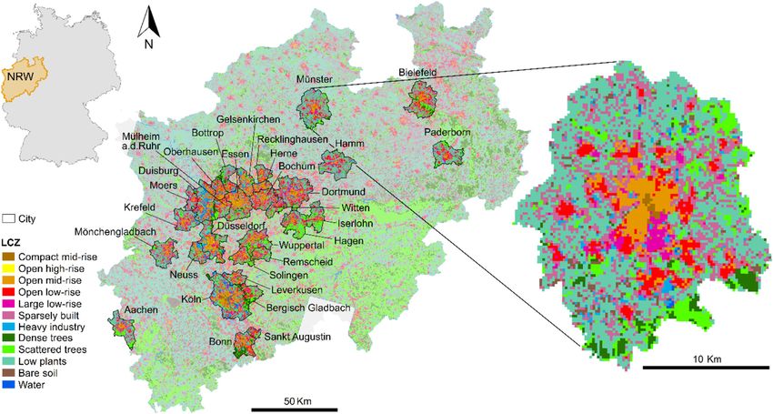
2012). Out of the 17 original LCZ classes, 12 were present in the region Source Type Description No. of
variables
(Fig. 1). The spatial pattern describes the distribution of phenomena
across space, e.g., concentration, dispersion, clustered patterns, etc. Remote Bands Mean and standard deviation of the pixel 10
sensing values. Data were atmospherically
(Getis & Paelinck, 2004). In particular, we refer to the arrangement of
corrected and haze removed.
urban structural types and land covers within cities. Texture Co- and occurrence features (local 60
For the classification of LCZ, we followed the protocol presented in standard deviation, average,
Tuia, Moser, Wurm, & Taubenböck (2017). We modelled LCZs on a grid homogeneity, entropy, dissimilarity,
composed of cells of size 200 × 200 m. In total, 89 variables were correlation, contrast and angular
moments).
3D Mean and standard deviation for both 5
nDSM and buildings only. The number of
buildings was also added as a feature.
Land Percentage of the area occupied by 4
cover buildings, trees, grassland and impervious
surfaces. The land cover is issued from an
object-based classification on a Rapid-Eye
mosaic (Montanges, Moser, Taubenböck,
Wurm, & Tuia, 2015).
GIS Roads Total line length for highway, primary, 7
secondary, tertiary roads, residential streets,
streams and rivers, smoothed with a
Gaussian kernel at the cell level.
POIs Counts for POIs cafes, restaurants and rail 3
stations, smoothed with a Gaussian kernel
Fig. 1. Summary of the LCZ classes present in NRW (from Stewart & Oke,
at the cell level.
2012). LCZs 2 to 10 are built-up classes, LCZs A to G land cover types.
3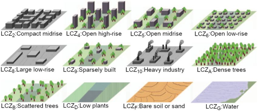
M. Sapena et al. Computers, Environment and Urban Systems 85 (2021) 101549
the metrics as the mean divided by the standard deviation, in order to 4. Results
obtain comparable regression coefficients and avoid influence of mea
surement units. 4.1. Spatial analysis of cities
When working with spatial metrics and a great diversity of structural
types, it is common to find redundant information since metrics depend In Table 3 we present the composition of the training/test sets and
on similar variables, cover similar spatial patterns, or can be comple the per-class and overall accuracies obtained for the LCZ classification.
mentary to each other (Reis, Silva, & Pinho, 2015; Schwarz, 2010). Per-class accuracy is given by the user’s and producer’s accuracy, where
Therefore, feature selection is a fundamental step (Genuer, Poggi, & the number of correct classified cells in a class divided by the total
Tuleau-Malot, 2015), as the high correlation of features may introduce number of cells classified as that class is the user’s accuracy (commission
noise in the process and affect the accuracy of results. In particular, error), and if divided by total number of cells of a class in the ground
regression models need the independence of predictors to minimize the truth is the producer’s accuracy (omission error) (Congalton, 1991). The
multicollinearity, which makes the model unstable. We followed three region was split in two parts (North and South) and training was per
consecutive approaches for the objective selection of metrics. First, we formed on the Northern region, while testing was performed on the
discarded the non-discriminative spatial metrics, those with a coefficient Southern to avoid positive biases related to spatial co-location of cells.
of variation lower than 5%. Second, we conducted a correlation analysis We obtained an overall accuracy of 83%, which is slightly lower than in
to identify redundancies in the spatial information. We omitted those Tuia, Moser, Wurm, & Taubenböck (2017), most probably due to the
metrics showing strong correlations to others (Pearson correlation co larger amount of testing samples used in this study. With the exception
efficient > 0.8), keeping one metric per group of correlated metrics. of the LCZ2 “Compact midrise” class and the LCZ5 “Open midrise” all the
Third, we applied a recent method proposed by Genuer, Poggi, & other classes are classified with more than 70% accuracy. Moreover, the
Tuleau-Malot (2015), called Variable Selection Using Random Forests average accuracies of 76.5% and 82.7% also show that the errors are not
(VSURF) that selects a specific subset of metrics adapted to each socio- systematic on the small classes. In Fig. 2 we illustrate the LCZ classifi
economic variable. This is based on measuring the relevance of every cation for the 31 sample cities in NRW. The detailed example of the city
metric in relation to each socio-economic variable using a random forest of Münster reveals how the structural variety of the built and natural
regression. We kept one subset of metrics for each socio-economic var landscape is captured by the LCZ classification.
iable (the different subsets of selected metrics are reported in Table 4). Concerning the spatial metrics, in total 22 global metrics per city and
24 class metrics per LCZ and city were calculated. Since our classifica
3.2. Estimating socio-economic and spatial pattern links tion map had 12 LCZ classes, 310 metrics were obtained at city level.
After the correlation analysis, a reduced subset of 72 uncorrelated
A model was obtained for each socio-economic variable from Table 1 metrics remained. This subset was the input in VSURF for each socio-
applying stepwise multiple linear regression analysis, using the subset of economic variable, obtaining one group of metrics per socio-economic
spatial pattern metrics previously selected as independent variables. We variable with sizes between 19 and 31 metrics (Table 4). This output
applied a min-max normalization transforming the socio-economic was part of the input in the following section as explained below.
variables in a range between zero and one as follows: zi = (xi-min(x))/
(max(x)-min(x)), where x = (x1, …,xn), xi is the ith original value and zi is 4.2. Models of socio-economic variables
the normalized value. For education, health, housing, affordability,
transport, and commuting the normalization was inversed and thus, In Table 5 we show the results of the eight fitted models, one for each
higher values mean better conditions for all variables. The number of socio-economic variable. The numerical goodness-of-fit indicators show
independent variables was restricted to a maximum of four spatial that the models are statistically significant (p-value < 0.05) and explain
metrics to avoid overfitting, considering the limited number of obser from 43% to 82% of the variability (R2) of the socio-economic variables
vations (cities) in our dataset. The residuals were tested for normality by means of the spatial structure of cities, with RMSEs ranging from 0.10
using the Shapiro-Wilk test (Shapiro & Wilk, 1965), and for statistical to 0.17. The values of the model of housing were normalized with a
significance by requiring p-values to be lower than 0.05. Leave-one-out logarithmic transformation to obtain a normal distribution of the re
cross-validation was employed to evaluate the models. We estimated siduals and improve the adjustment (Table 5). The spatial metrics
the root mean squared error (RMSE) and the coefficient of determination included in each model and their associated coefficients allow inter
(R2) to summarize the proportion of variance explained by the model, preting which and to what extent spatial patterns explain the modelled
and thus the goodness-of-fit. variable (Table 5). As they are all standardized to z-scores prior to the
To verify whether the level of ‘quality of life’ in cities is reflected in analysis, their direct contribution is represented by the regression
their urban spatial structure we conducted a two-step analysis: (1) we coefficients.
used the k-Means clustering method to group cities according to their The relationships we found between the spatial structure of the cities
values of socio-economic variables, representing variables from five in this region and the socio-economic variables are as follows: cities with
dimensions of quality of life considered in our study (Table 1), out of a better level of education have less open, and thus more continuous,
nine (Eurostat, 2017). Using the Elbow method (Ketchen & Shook, built-up (PU), however, the distribution of open midrise is more scat
1996) we found an appropriate number of groups. Consequently, we tered (DEMp5), dense tree patches are furthest away from the city center
created and described four clusters that group cities based on their socio- (DimRA), and there is a higher density of open high-rise buildings (DC4).
economic similarities. Moreover, we represented the ‘quality of life’ for In terms of health, the model relates a lower death rate in cities with a
each city and group using star plots, as well as the average of the region, fragmented and distant distribution of sparsely built (DEM9) and scat
which facilitates the interpretation of the different groups of cities; (2) tered tree (DEMB) patches. Conversely, larger and less fragmented areas
we applied a stepwise discriminant analysis for selecting a relevant and of heavy industry (IS10) are usually present in cities with higher levels of
reduced set of spatial metrics - based on their significance - that better death rates. On the one hand, a compact shape of open midrise (C5),
separates the cities into these groups. Afterwards, the values of the scattered from city centers towards the suburban areas (DEP5) with a
spatial metrics, and thus the spatial structure of cities, were interpreted compact midrise core (TM2) is related to lower prices of housing. On the
for each group. other hand, income is higher in cities with bigger extensions of open low-
rise (TEM6), clustered dense trees (ISA), and contiguous areas of sparsely
built with very few open areas (P9). Regarding the ability to pay for
housing based on income, the model is similar to housing model (TM2
and C5), except that the affordability is inversely proportional to the
4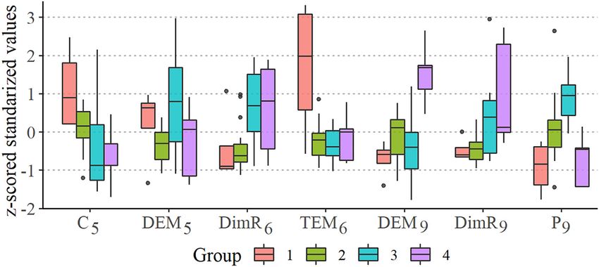
M. Sapena et al. Computers, Environment and Urban Systems 85 (2021) 101549
Table 3
Numerical results of the LCZ classification and number of samples used for train/test steps. User’s and producer’s accuracy and global statistics.
Code LCZ No. samples (train/test) User’s accuracy Producer’s accuracy
Land cover LCZ A Dense trees 186 / 114 76.99% 76.32%
LCZ B Scattered trees 118 / 107 74.77% 74.77%
LCZ D Low plants 169 / 131 81.41% 96.95%
LCZ F Bare soil or sand 108 / 192 97.33% 94.79%
LCZ G Water 194 / 106 98.85% 91.13%
Built-up LCZ 2 Compact midrise 82 / 39 45.59% 79.49%
LCZ 4 Open high-rise 13 / 26 100% 3.85%
LCZ 5 Open midrise 124 / 72 67.95% 73.61%
LCZ 6 Open low-rise 152 / 48 88.10% 77.08%
LCZ 8 Large low-rise 100 / 101 91.01% 80.20%
LCZ 9 Sparsely built 153 / 55 81.67% 89.10%
LCZ 10 Heavy industry 148 / 192 88.62% 90.83%
Average accuracy – 82.69% 76.51%
Overall accuracy – 83.08%
kappa – 0.81
Fig. 2. Location of NRW in Germany (left). Result of the classification for the NRW region highlighting the classification in the analyzed cities (middle). Detailed
example of the classification for Münster (right).
fragmentation of open low-rise (IS6). Therefore, the ability to pay is 4.3. Categorization of cities
lower in bigger cities with a compact midrise core surrounded by frag
mented clusters of open low-rise structures. Fig. 3 shows the clustering of cities according to their socio-economic
In relation to the economic aspects (employment), open low-rise similarities using the normalized values of six socio-economic variables
located towards the periphery of the city (DimR6) and a fragmented (we excluded the share of journeys to work by car or motor cycle since
and distant distribution of sparsely built (DEM9) are characteristic of statistics were available only from 29 cities and the ability to pay for
cities with higher employment rate, moreover, LCZ patches are bigger, housing since housing and income were included instead). The indi
which means more continuous LCZ classes and, in general, less isolated vidual plots show the location of cities by means of the bi-dimensional
small patches (TEM). Concerning transport, fragmented cities (TEM) in spaces defined by each pair of socio-economic variables. Cities are
small continuous clusters (GC), with higher proportion of sparsely built identified by means of a number and color. The map depicts how cities
areas (DC9) and a lower number of large low-rise areas (DO8) commute and groups are distributed in the region. It can be seen that the first
more by car or motor cycle. Meanwhile, citizens living in cities associ group (green) is easily identified by means of income and commuting
ated with more compact areas of sparsely built structural type (C9) levels (income and commuting plots in Fig. 3). While education discerns
commute more out of the city (commuting). The way in which open low- the second group (blue, education plots in Fig. 3), the identification of
rise is allocated affects commuting patterns. The higher the number of the third group (orange) is not straightforward. However, the fourth
compact clusters (LPF6 and IS6) the more the commuting proportion. (red) can be identified by means of death rate, price of buying an
apartment and employment rates (health, housing, and employment
5
M. Sapena et al. Computers, Environment and Urban Systems 85 (2021) 101549
Table 4
Description of the selected spatial metrics (independent variables in the models from Table 5). The significant relations between metrics and socio-economic variables
according to VSURF, are shown in the intersection of the rows and columns. The characters show whether metrics computed at the class level (with their LCZ short
codes, see Table 3), at the city level (X), or lack of relation (− ). Formulas can be consulted in Sapena and Ruiz (2015, 2019). Patch means a group of contiguous pixels
with the same LCZ class.
Spatial metric Description Education Health Housing Income Affordab. Employ. Transport Commut.
Compactness (C) Measures the shape complexity of the LCZ class. – F A,F,5,9 – A,F,5,9 A,F,5,9 A,5,9 A,F,5,9
Class density (DC) The ratio between the LCZ class area and city area. 2,4,10 D, A,F, 6 A,F, 9 6,9 6
F,5,9 G,2,5,6,9 G,2,5,6
Density-diversity Sum of the ratios between the areas of every LCZ class – – X – – X X X
(DD) and the largest LCZ class. Informs about the richness
and heterogeneity.
Patch nearest Mean Euclidean distance between the nearest patches B,5 A, 10 9 10 5,9 5,9 9
neighbor (DEM) from the same LCZ class (km). B,8,9
Pixel nearest Mean Euclidean distance between the nearest pixels A,5,6 D,6 8 A A D – A
neighbor from the same LCZ class (km).
(DEMp)
Wei. Standard Area-weighted mean distance of patches from the – A,5 – 5 A,6 A D,6 8
distance (DEP) same LCZ to their centroid (km). Informs about the
concentration degree.
Object density The number of patches of the same LCZ divided by the 6,9 B,5,6 D,5 – D D,5 D,8 D,5
(DO) area of the city.
Urban density The ratio between the built-up area (LCZ2-10) and the – X – – – X X –
(DU) city area.
Radius dimension Measures the centrality of the LCZ classes with respect A,6,9 A,B,G A,6,9 G,8,9 6,9 6,9 A,6,9 6,9
(DimR) to the city center given.
Coherence deg. The probability that two random points are in the X – X – X X X X
(GC) same patch in a city.
Shape index (IF) A normalized ratio of patch perimeter-area in which 2 – 2 – 2 – 2 2
the complexity of patch shape is compared to a square
of the same size.
Splitting index (IS) The number of patches when dividing the LCZ class X,G F,10 X,6 A,6 X,6 X,6 X,6 X,6,10
into equal size parts with the same division.
Leapfrog (LPF) The proportion of isolated pixels with respect to the 6 5,8 A,B A 5,6 – 5,6 5,6
entire LCZ class.
Urban− /porosity The ratio of open space (area of holes within the built- X – 5,9 X,9 5 – 5 5
(PU, P) up area or LZC class) compared to the city or LCZ area
(Reis, Silva, & Pinho, 2015).
Contrast (RCB) The sum of the segment lengths of pixels adjacent to D D A X – X,D D –
different LCZ, divided by the perimeter.
Effective mesh size Measures the connectivity. Low values mean 2 6,8 2,8 2,6,8 2,6,8 X,2,8 X,2,8 X,6
(TEM) fragmentation (ha).
Object mean size Average size of the patches from a LCZ class (ha). 2,4,9 F,G,9 2 G,2,4 F,2 – 2,9 2
(TM)
Table 5
Multiple linear regression models for the normalized socio-economic variables, where higher values mean better conditions for all variables (dependent variables, DV),
using the spatial metrics (independent variables (IV) in bold, with the LCZ class in the subscript). The intercept, coefficients of IV, leave-one-out cross-validation
coefficient of determination (R2), the root mean square error (RMSE), the p-value of the model, and the number of observations or cities (Ob) are shown. The acronyms
of LCZ and spatial metrics can be found in Tables 3 and 4, respectively.
DV Intercept IV 1 IV 2 IV 3 IV 4 R2 RMSE p-value Ob
6
Education 0.407 0.159⋅DEMp5 0.119⋅DimRA − 0.110⋅PU 0.077⋅DC4 54.87 0.174 7.7⋅10− 31
6
Health 0.389 0.130⋅DCF 0.102⋅DEMB 0.081⋅DEM9 0.081⋅IS10 49.78 0.175 9.9⋅10− 31
5
Log(housing) 0.536 0.138⋅C5 0.093⋅P9 − 0.060⋅TM2 0.057⋅DEP5 50.61 0.151 1.2⋅10− 31
5
Income 0.560 0.112⋅TEM6 − 0.092⋅ISA − 0.057⋅P9 43.4 0.165 2.7⋅10− 31
6
Affordability 0.580 − 0.088⋅TM2 0.076⋅C5 − 0.067⋅IS6 53.98 0.153 3.9⋅10− 31
7
Employment 0.281 0.108⋅DimR6 0.108⋅DEM9 0.093⋅TEM 56.84 0.157 2.0⋅10− 31
6
Transport 0.457 0.236⋅TEM − 0.149⋅GC 0.114⋅DO8 − 0.057⋅DC9 51.22 0.166 5.1⋅10− 29
11
Commuting 0.637 − 0.222⋅C9 0.100⋅LPF6 0.078⋅DEM9 − 0.059⋅IS6 82.29 0.101 7.4⋅10− 31
plots in Fig. 3). comparison with the rest of the groups, and a close to 15% commute out
The interpretation of groups by their mean values (i.e.: group cen of the city. Group 3, which most closely approximates to the mean values
troids using the non-scaled socio-economic variables, Table 6), shows of the region (Table 6), clusters seven cities; in this group the education
that group 1 is formed by four cities with medium and low rates of level and health are medium, the price of buying an apartment is high in
mortality and low-education, the prices of buying an apartment are the contrast with the lower income levels (i.e., low capacity to pay for
lowest in contrast to the highest income levels (i.e., the capacity to pay housing), however, the employment rate is medium-high and there are
for housing is higher), however, the low employment is balanced by the low commuting rates. Finally, group 4 gathers five cities with the lowest
highest commuting level to work out of the city. Group 2 accounts for the proportion of the low-educated population, lower rates of mortality, and
majority of cities (15 out of 31). This group is characterized for having the highest prices for buying an apartment accompanied by high-income
lower education and employment together with higher death rates, the values; however, the huge discrepancy suggests housing prices are less
prices for buying an apartment and the income are medium-low in affordable, the employment rate is the highest of the region and the level
6
M. Sapena et al.                                                                                                 Computers, Environment and Urban Systems 85 (2021) 101549

Fig. 3. Clustering of cities into four groups using the scaled socio-economic variables. The individual scatter plots show: the location of the cities according to each
pair of socio-economic variable (row and column, e.g.: the top-left plot corresponds to ‘education’ and ‘health’), the centroid of each group, and the distance of cities
to their centroid. The map locates spatially the clusters and combined with the table identifies the cities (identification number, group and name of the city). It
compares cities relatively based on to their socio-economic performance and groups them according to their similarities.

Table 6
Mean of non-scaled socio-economic variables (centroids) and number of cities per group. The last row shows the mean values of the NRW region.
  Group            Cities     Education (%)         Health (n◦ /1000)        Housing (€)         Income (€)        Employment (n◦ /1000)          Commuting (n◦ /1000)

  1                4          27.59                 9.92                     91,875              23,975            426.01                         215.27
  2                15         37.24                 11.89                    91,933              20,900            421.49                         148.49
  3                7          29.44                 11.36                    104,000             19,700            498.79                         112.94
  4                5          26.37                 9.01                     134,400             22,200            686.05                         97.82
  NRW              31         32.48                 11.05                    101,500             21,235            482.20                         140.91

                                                                                    7
M. Sapena et al. Computers, Environment and Urban Systems 85 (2021) 101549
Fig. 4. Multi-dimensional quality of life star plots of cities by group. Values are relative, as the socio-economic variables were min-max normalized between zero and
one. For education, health, housing, and commuting the normalization was inversed and thus, higher values mean better conditions. The legend (top right) shows the
maximum value of each socio-economic variable, equal to one, and its name related to the position and color. The mean values of the NRW region are represented in
the bottom right. The gray background shows the maximum reachable value.
of commuting out of the city is the lowest. relationships, we selected the spatial metrics that best identify these
By representing the cities multi-dimensionally using the socio- groups. We started from the subset of metrics selected with the VSURF
economic values by means of star plots (Fig. 4), the shape of each city method. Five spatial metrics for three structural types were the most
becomes an indicator of its ‘quality of life’ (here based on five di influential in terms of grouping cities into different levels of quality of
mensions), the more complete (i.e., the area of the gray circle is covered) life. Those metrics were: the distance between sparsely built and open
the better. Group 1 shows high levels of commuting out of the city, ed midrise structures patches within the city (DEM9 and DEM5), the num
ucation, health, house affordability, and income, but very few employ ber of open areas within the sparsely built patches (P9), the connectivity
ments (work place-based). This shape can be related to satellite cities and size of open low-rise patches (TEM6), the compactness of open
with good quality of life (regarding education, health and living con midrise (C5), and the centrality (proximity to the city center) of sparsely
ditions) but a less desirable situation in terms of sustainability due to the built and open low-rise (DimR9 and DimR6). The spatial patterns that
high commuting shares, to balance against the low employment rate. In better differentiate between the derived levels of quality of life can be
group 2 we find the lowest values of education and health in the region, analyzed by representing the values of these metrics for each socio-
commuting is medium-high and housing is affordable compared to in economic group in box-and-whiskers plots (Fig. 5). The spatial pat
come levels, however employment is quite low. There are similarities terns that better represent the cities in group 1 are the presence of the
with the first group in the values of employment and housing, however, biggest continuous areas of open low-rise, the highest compact shapes of
the analysis of the rest of variables suggests that this group has the open midrise patches but spatially scattered, and the compact distribu
lowest quality of life relative to the entire region. Group 3 presents the tion of sparsely built close to the city centers. For group 2, the metrics
lowest values of income in the region, and health is slightly lower than portray an even distribution of the sparsely built areas through the city,
that of the mean NRW value. However, the remaining socio-economic with fragmented and centralized open low-rise. Group 3 shows open
variables are quite close to the mean values, which may suggest a midrise structures scattered across the city, plus high values of open
quality of life close to the NRW average. Finally, group 4 has the lowest areas in the sparsely built environment, close to each other but farther
values of commuting out of the city, while education, health, employ from the urban cores, pointing that these urban structures are located in
ment and income are considerably high and, as a counterpart, housing is the surrounding areas of the city centers that are mainly occupied by
less affordable. Additionally, this can be considered the most sustainable high and medium rise types. Finally, cities in group 4 are especially
group in terms of commuting shares. Thus, according to the analyzed characterized by a compact nucleus of open midrise structures, with
dimensions, it could be objectively said that it shows the highest quality irregular shape, combined with fragmented distribution of sparsely built
of life in the region. far from the urban cores, probably as they are located in the outskirts of
The spatial structure of urban spaces, as mentioned in the intro the city, as well as the fragmented and decentralized distribution of open
duction, is related to this measured ‘quality of life’. To explore such low-rise (Fig. 5). That is, cities in group 4 have a compact urban core
8M. Sapena et al. Computers, Environment and Urban Systems 85 (2021) 101549
Fig. 5. Box-and-whiskers plot illustrating the standardized values of the spatial metrics for each socio-economic group of cities. Where: C = compactness, DEM =
patch nearest neighbor, DimR = radius dimension, TEM = effective mesh size, and P = porosity. The subscript shows the LCZ: 5 = open midrise, 6 = open low-rise
and 9 = sparsely built.
becoming gradually less compact as the distance to the core increases, higher automobile dependency in low-dense Italian cities. The positive
eventually with low-dense structures located in the outskirts. For relation of low-dense cities with higher incomes and commuting shares,
example, Münster (detailed example from Fig. 2) present this spatial especially by car or motor cycle, is likely to be linked to preferences of
pattern, with a compact midrise core (orange), with decentralized high-income households to live in less dense areas despite the higher
fragmented clusters of open low-rise (red) intermixed with a scattered travel cost. Additionally, the proportion of employment showed a pos
and isolated distribution of sparsely built (pink). itive relation to the homogeneity of structural types, they seem to be
more organized, that may suggest that cities with more jobs are planned
5. Discussion in a more uniform spatial distribution, with the exception of the sparsely
built that tends to be more fragmented in these cities. Other authors also
Our study in the cities of North Rhine-Westphalia in Germany shows found relationships between spatial metrics and percentages of land uses
the interrelation of urban spatial structure with quality of life di with employment sector statistics (Ghafouri, Amiri, Shabani, & Songer,
mensions. Our findings show that the education, mortality, income, 2016).
employment, and other quality of life indicators can be partially The socio-economic variables used in this study cover several di
explained by urban spatial pattern metrics extracted from urban struc mensions of quality of life (Eurostat, 2017). Therefore, grouping cities
tural types and land covers. No more than four metrics were needed to according to the socio-economic variables allowed us identifying
explain more than 40% of the variability of the socio-economic levels in various levels of quality of life within the analyzed cities. One group
cities with a similar economic and historical background for a given presented the lowest level in the region, but it does not necessarily mean
time. For example, the level of education tended to be better in more that the quality of life is poor because we are comparing relative values.
compact cities but also in cities with low-dense structures (i.e., open On the contrary, two groups stood out for having better levels of quality
low-rise and sparsely built), which correspond to major cities and their of life. These groups differ in commuting patterns, housing affordability,
satellite cities in NRW, respectively. This link can be related to higher- and employment rates, and coincide with major cities and satellite cities.
educated people moving to bigger cities seeking better job opportu Despite having a good quality of life, satellite cities here identified with
nities, and eventually moving to satellite cities. This seems to differ with low-dense built structures, are unsustainable in terms of commuting and
a study where higher education levels were found in low-dense urban transport choices, besides low-dense cities are more inefficient in the use
areas against high-dense areas in North America (Batchis, 2010). Cities of land, energy and resources (Bhatta, 2010). We also found common
with distant agglomerations of sparsely built areas and vegetation, spatial patterns related to the built-up structural types in cities that had
combined with fewer and more scattered industry areas showed fewer similar levels of quality of life, which again suggests the two-sided
death rates. In this sense, Oliveira (2016) compiled case studies that impact of spatial structure of cities on their socio-economic levels. We
related walkability, diversity of land uses, and urban form with an should note here that this specific morphology found for cities in NRW
improvement in health habits. The positive relation between death rate for a given date do not necessarily have the same relations in other areas.
and bigger areas of heavy industry, besides higher shares of death in Context is - as Tonkiss (2013) argues - all in this debate. However,
cities from groups 2 and 3, could be related to the fact that most of these similar correlations between urban spatial structures and economical
cities are located in the highly industrialized Ruhr region, where death functions have been previously discussed in the literature. For instance,
rates are high (Kibele, 2012). Apartments in cities of NRW with midrise Mouratidis (2018) found a positive relation between social well-being
structures (compact in the core and open towards the suburbs) and and high density, short distances to the center, and land use diversity.
patches of dense tree are prone to be more expensive. We also found that Venerandi, Quattrone, & Capra (2018) modelled deprivation to popu
income is measured higher in cities with a larger share of continuous and lation density, higher proportion of bare soil and regular street patterns,
homogeneous areas of very low-dense built-up areas (i.e. sparsely built while other authors predicted indicators of wealth, poverty and crime
and open low-rise structural types), a spatial pattern that is especially through satellite data (Irvine, Wood, & McBee, 2017). Studies relating
seen in the satellite cities in NRW. Similarly, we found that commuting urban spatial structures with socio-economic values are usually focused
out of the city is higher in cities with more clusters and more compact in single dimensions, such as education, poverty, transport, air pollu
areas of these low-dense built-up structural types, and the share of tion, health, energy consumption, etc. (e.g.: Batchis, 2010; Duque et al.,
people choosing to commute by car or motor cycle is higher in less 2015; Hankey & Marshall, 2017; Sandborn & Engstrom, 2016; Wurm
diverse and low-dense cities, which could be related to more mono et al., 2019). Only a few of them analyze various indicators (e.g.: Irvine,
functional and dispersed cities. This tendency is widely discussed in the Wood, & McBee, 2017; Sapena, Ruiz, & Goerlich, 2016) or combine
literature, for example, Travisi, Camagni, & Nijkamp (2010) found them (Tapiador, Avelar, Tavares-Corrêa, & Zah, 2011). In contrast, we
9M. Sapena et al. Computers, Environment and Urban Systems 85 (2021) 101549
tackled several aspects individually related to the quality of life and also of cities and their socio-economic levels, in this paper we quantified
in a combined way. We found that cities with a higher socio-economic their relationships by means of statistical models. This supports the
status in NRW have a core with spatially compact midrise structures, hypotheses that assume that the spatial structure of cities reflects social
while on the periphery there are small groups of low-rise structures and and economic indicators of their inhabitants, and eventually influence
sparsely structures disaggregated with a high proportion of open green their quality of life. The applied methodology can be used as a tool to
spaces. However, we are fully aware that the urban spatial structure of obtain empirical evidences as well as learning from past trends and
cities does not define or fully explain their success, since there are many understanding the present to design a better future.
other factors that play an important role. However, in the region
analyzed, cities with similar spatial appearance also had similar socio- 6. Conclusions
economic levels; this is a strong indication that the spatial structure of
the cities do influence socio-economic performance. It should also be The spatial structure of urban spaces is related to the quality of live
recalled that correlation does not imply causation, and thus the variation and sustainability of our cities. This is clearly confirmed by this analysis
of a spatial pattern does not necessarily improve the socio-economic of cities in NRW. We extracted the spatial structure of cities using spatial
level of a certain area, although, it will certainly alter its state (Lehrer pattern metrics from a LCZ classification based on machine learning
& Wieditz, 2009; Williams, 2014). algorithms applied to multimodal geospatial data. These attributes
We also faced some limitations. We based the relations on a large and explained the variability of quality of life related indicator, which are
consistent set of variables. However, a comprehensive set of variables is linked to six out of seventeen SDGs. Moreover, grouping cities into
inexistent which means that we are not able to depict the manifold in different levels of quality of life showed common spatial patterns within
terrelationships holistically. Moreover, it is worth noting that we did not the groups. We ascertained that the spatial structure of cities has a strong
include external influences in the models, such as policies, individual influence on their socio-economical functions, but does not fully deter
historical background, etc. While of course, every city is unique, the mine them.
overall urban spatial structure of the analyzed cities is comparable to a In times of increasing availability of socio-economic and spatial data
certain extent, thus reducing these influences. However, when con (e.g. from remote sensing) in ever-increasing spatial resolutions, there is
ducting a global analysis, externalities should be considered, as well as a huge demand for systematic research in this direction. Of particular
measuring the spatial stratified heterogeneity (Wang, Zhang, & Fu, interest is research that systemizes these relations in dependence of
2016) to test whether the variables are distributed unevenly across context, that is policies, culture, demography, etc., for a more general
different parts of the study area, in which case it would be convenient to and quantifiable knowledge of the influence of the urban spatial struc
perform different models. Besides, it was not possible to model some ture on socio-economic parameters of cities and their people – this paper
socio-economic factors such as the ‘proportion of economically active testifies to this.
population’ or the ‘share of persons at risk of poverty after social Although this study accounts for cities in NRW in a specific period,
transfers’ with the spatial distribution of LCZs, and thus they were not and thus is not globally representative, results show a trend that is worth
included in the analysis. Regarding the data used in this study, it is investigating further. This is feasible due to the growing availability of
important to mention the following: on the one hand, the urban spatial data for both local and global levels. Moreover, the methods applied in
patterns of cities were extracted by means of spatial pattern metrics. this study are directly transferable to other regions and datasets, which
When working with spatial metrics, diminishing redundancies by would broaden the analysis and derived conclusions. Additionally, the
removing duplicated information and the selection of the most signifi increase of the temporal scale would allow gaining knowledge of how
cant variables is of great importance (Sapena & Ruiz, 2019; Schwarz, urban growth affects cities and urban areas spatially and socio-
2010). Another consideration is that the accuracy and spatial resolution economically, and inversely the influence of socio-economic policies
of the image classification (here measured with 83% overall accuracy) and evolution on the urban growth patterns, as well as quantifying their
affects to the spatial metrics, this fact needs to be considered when interrelationships. The analysis of the relationships of urban developing
extracting conclusions of such studies. On the other hand, the socio- processes, e.g. the effect of city design choices on urban fabric, is of high
economic data used in this study have a great potential for compara interest for future research and will provide a valuable source of infor
tive studies in Europe, but as mentioned, the average values at city level mation for supporting policy makers and city planners to ensure the
disregard internal socio-economic variations assuming that cities are quality of life and sustainable development in urban areas.
homogeneous. Another limitation is the use of only five aspects of
quality of life based on eight indicators, instead of a larger subset of Declaration of Competing Interest
socio-economic variables to enrich the analysis. Although these vari
ables were able to represent a significant part of the different levels of None.
quality of life in the region, we were subject to the availability of data.
Moreover, data quality and spatial units should be considered (Schwarz,
Acknowledgements
2010; Venerandi, Quattrone, & Capra, 2018). Whereas remote sensing
and GIS derived products, such as the LCZs classification, have no
This research has been partially funded by the Spanish Ministerio de
boundary or time-scale limitations, socio-economic statistics are usually
Economía y Competitividad and European Regional Development Fund
restricted by administrative boundaries and census dates. Nevertheless,
(CGL2016-80705-R) and by the Swiss National Science Foundation
there is a recent tendency to provide these data in a different format,
(PP00P2-150593).
such as gridded datasets that swap irregularly shaped census boundaries
to a regular surface (EFGS, 2019). These new datasets will serve as an
References
opportunity to conduct studies that are not restricted by administrative
boundaries. Abrantes, P., Rocha, J., Marques da Costa, E., Gomes, E., Morgado, P., & Costa, N. (2019).
The quality of life of the population and the sustainable development Modelling urban form: A multidimensional typology of urban occupation for spatial
of urban areas are in the spotlight (OECD, 2017). Improving the un analysis. Environment and Planning B: Urban Analytics and City Science, 46(1), 47–65.
Anderson, W. P., Kanaroglou, P. S., & Miller, E. J. (1996). Urban form, energy and the
derstanding of the spatial structure of urban areas, the demographic, environment: A review of issues, evidence and policy. Urban Studies, 33(1), 7–35.
social and economic levels of these areas and their interrelations con Batchis, W. (2010). Urban sprawl and the constitution: Educational inequality as an
tributes to planning the development of cities with a view to meeting the impetus to low density living. The Urban Lawyer, 42, 95–133.
Bechtel, B., Alexander, P. J., Böhner, J., Ching, J., Conrad, O., Feddema, J., … Stewart, I.
global policy objectives set out in the New Urban Agenda (UN-Habitat, (2015). Mapping local climate zones for a worldwide database of the form and
2016). In order to unravel the interactions between the spatial structure function of cities. ISPRS International Journal of Geo-Information, 4(1), 199–219.
10You can also read