Constraint-Following Approach for Platoon Control Strategy of Connected Autonomous Vehicles

Hindawi
Journal of Advanced Transportation
Volume 2022, Article ID 8623410, 15 pages
https://doi.org/10.1155/2022/8623410

Research Article
Constraint-Following Approach for Platoon Control Strategy of
Connected Autonomous Vehicles

 Mengyan Hu , Ying Gao , Xiangmo Zhao, Bin Tian , and Zhigang Xu
 School of Information and Engineering, Chang’an University, Xi’an, Shaanxi, China

 Correspondence should be addressed to Ying Gao; gaoying888@chd.edu.cn

 Received 22 November 2021; Revised 11 January 2022; Accepted 15 January 2022; Published 7 February 2022

 Academic Editor: Zhenzhou Yuan

 Copyright © 2022 Mengyan Hu et al. This is an open access article distributed under the Creative Commons Attribution License,
 which permits unrestricted use, distribution, and reproduction in any medium, provided the original work is properly cited.

 The current platoon control strategies of connected autonomous vehicles (CAVs) focus on controlling the fixed intervehicle
 distance, i.e., the string stability of the platoon system. Here, we aimed to design a CAV platoon control strategy based on a
 constraint-following approach to solve the problem of platoon starting. As the resistance of the vehicle during driving varies with
 time, this study regarded the CAV platoon system as a changing dynamic system and introduced the Udwadia–Kalaba (U–K)
 approach to simplify the solution. Apart from adding an equality constraint, unlike most other studies, this study imposed a
 bilateral inequality constraint on the intervehicle distance between successive CAVs to prevent collisions. Meanwhile, a dif-
 feomorphism method was introduced to transform the bounded state into an unbounded state. The proposed control strategy
 could render each CAV compliant with both the original imposed bilateral inequality constraint and the equality constraint. The
 former avoids collisions, and the latter indicates the string stability of the designed CAV platoon system. The effectiveness of the
 proposed controller was verified by numerical experiments. The gap errors tend to converge to zero, which is not amplified by the
 propagation of traffic flow.

1. Introduction the surroundings and govern the speed of the vehicle to
 improve ride comfort. V2V and vehicle-to-infrastructure
With the increasing growth of the automobile industry, (V2I) communications enable CAVs to extend their visi-
urban transportation networks are experiencing significant bility [10]. When a group of CAVs travels with a short
issues in a variety of areas. It can easily cause speed intervehicle spacing or gap, a platoon is formed [11]. CAVs
breakdown, traffic flow oscillation, and congestion in con- can share information and adopt more aggressive control
verging portions of traffic flow in fragile highway systems for strategies, thereby yielding better traffic throughput and
many cars [1]. In recent years, public interest in research on increasing traffic efficiency [12, 13]. In addition, driving in a
intelligent transportation systems has grown faster. platoon can change the aerodynamic forces on vehicles,
 Autonomous vehicles are designed to free drivers from thereby improving fuel economy [14–16]. Compared to
driving tasks and are expected to improve traffic safety and individual autonomous vehicles, CAVs in a platoon have
efficiency when connected through vehicle-to-vehicle (V2V) greater potential to improve traffic performance because
communication, i.e., connected autonomous vehicles they can share information and coordinate their behavior to
(CAVs). They also have great potential for dealing with ensure shorter intervehicle distances safely [4, 17–19], as
traffic problems [2, 3]. Autonomous vehicles that use ad- illustrated in the field tests [20, 21]. With V2I communi-
vanced sensing, communication, and control technologies cation between roadside units and autonomous vehicles,
have the potential to increase road capacity and improve traffic stability can be improved [22]. Hence, the study of the
traffic operations [4–6]. An adaptive cruise control system, CAV platoon system is of great significance.
one of the earliest autonomous vehicle systems, has already The earliest concept of an autonomous vehicle platoon
entered the market [7–9]. It uses on-board sensors to detect system was proposed in 1939 [23], however, it has aroused

2 Journal of Advanced Transportation

great interest since 1986 [24]. Thereafter, an increasing string stability of the CAV platoon under the premise of
number of studies on intelligent transportation systems have sufficient safety. To this end, we, firstly, formulated a
been conducted. Among them, control design is one of the nonlinear longitudinal dynamic model for each vehicle,
most important issues in intelligent transportation systems. considering the possible time-varying uncertainties, and we
Stankovic et al. [25] proposed a decentralized overlapping obtained a multivehicle dynamic system. Subsequently, we
control law for the platoons of intelligent vehicle systems. In incorporated an equality constraint and a bilateral inequality
particular, they adopted a reduced-order observer and constraint into the dynamic system. The former was set to
feedback map to design the control law. Lee et al. [26] used a ensure that spacing error between the current platoon state
fuzzy sliding algorithm to build a platoon controller to and the final platoon state would converge to zero. The latter
compensate for the effect of uncertainty. Thus, the exact was adopted to restrict the intervehicle distance within an
models of vehicles are not required. Antonelli et al. [27] appropriate range during the entire process to guarantee
separated the control architecture into two task-oriented safety. The U–K approach was utilized to render an explicit
stages. Therefore, the vehicle kinematic model is required to control force for the specific dynamic system constructed in
construct the control law to complete the task. Ghasemi et al. this study. As the original U–K approach cannot handle
[28] proposed a hybrid controller consisting of a feedback inequality constraints, the diffeomorphism method [42] was
linearization controller and a decentralized bidirectional applied to free the inequality constraint by transforming the
controller for successive vehicles maintaining a constant bounded state to an unbounded state. Thus, the U–K ap-
space. Other recent studies can be found in [29–32]. Lee and proach could be used. Finally, the Lyapunov stability theory
Kim [33] present a control algorithm for a platoon of ve- was employed to verify the performance of the proposed
hicles. The headway distance to the preceding vehicle and its control strategy. We proved that the proposed control force
changing rate along with the velocity of the leading vehicle could render uniform boundedness (UB) and uniform ul-
are used to derive the headway control laws without using timate boundedness (UUB) performance for the unbounded
headway information from other vehicles. Desjardins and state. The main difference between this study and other
Chaib-Draa [34] proposed a novel approach for the design of works is that the complicated platoon control problem was
autonomous vehicle controllers based on modern machine- treated as a constraint-following problem, and the U–K
learning techniques, which used function approximation approach was used to simplify the solution of this specific
techniques along with gradient-descent learning algorithms problem.
as a means of directly modifying a control policy to optimize The remainder of this paper is organized as follows: the
its performance. To guarantee the string stability of a vehicle basic theory of the U–K approach is introduced in Section 2.
platoon, Kayacan [35] proposed a multiobjective H-infinity The platoon model of a specific situation considering pa-
control formulation for adaptive cruise control and coop- rameter uncertainty is detailed in Section 3. Subsequently,
erative adaptive cruise control structures. Wen et al. [36] longitudinal dynamic models for a CAV platoon are in-
proposed a useful string stable CCVP algorithm to guarantee troduced, and the control strategies based on the U–K
the string stability and zero steady-state spacing error for the approach are designed with and without parameter un-
platoon, where the controller gain of the platoon is further certainty in Section 4. The simulation experiments are
complemented by additional conditions. designed to verify the performance of the controllers, fol-
 Platoon control strategy as one of the most significant lowed by a discussion of the simulation results in Section 5.
aspects is studied by many researchers for decades. The Finally, the findings are concluded along with some future
motion of the CAV platoon in this study was regarded as a research directions in Section 6.
dynamic system because the aerodynamic resistance of each
vehicle varied continuously, and it was necessary to dy- 2. U–K Approach
namically adjust the tractive force of each vehicle to com-
pensate for the changing resistance to ensure the stability of In this section, we discuss the fundamental equations of the
the platoon system. To control the dynamic system, Udwadia U–K theory, which are the foundation of our research. This
and Kalaba [37] developed a constraint-following approach, theory can be divided into the following three steps [37]:
in which constraints are integrated into system dynamics in
the form of “constraint force” and introduced a series of
explicit and legible equations to solve the control law of a 2.1. Unconstrained System. In nature, all motions follow
dynamic system subject to equality constraints. Because of Newton’s second law, and the generalized form of the
its simplicity, the Udwadia–Kalaba (U–K) approach has equation of motion can be described as follows:
been applied to various dynamic control problems and has F � ma, (1)
shown good practicability [38–40]. However, the original
U–K approach was designed to cope with equality con- where F is the total force exerted on the system, m is the
straints. Hence, the problem of dealing with bilateral in- mass, and a is the acceleration.
equality constraints remains challenging [41]. The Newton equation connects the force, mass, and
 To summarize, this study investigated the platoon acceleration of the system. Lagrange introduced the concept
control strategy for CAVs in the context of longitudinal of generalized coordinates and used the D’Alembert prin-
motion. Our purpose was to design a CAV platoon control ciple to obtain an equation that is equivalent to Newton’s
strategy, apply it to the platoon starting, and ensure the second law. It is called the Lagrangian equation. The motion

Journal of Advanced Transportation 3

equation of U–K mechanics for an unconstrained system M(q, t)€ _ t) + Qc (q, q,
 q � Q(q, q, _ t), (7)
can be obtained by Newtonian or Lagrangian mechanics,
which can be written in the form of where Qc is the constraint force causing the change in ac-
 celeration, which can be regarded as a set of control forces
 M(q, t)€ _ t),
 q � Q(q, q, (2)
 acting on the unconstrained system.
where M is a positive definite inertia n × n matrix, q is the In the Lagrangian motion equation, Qc represents the
coordinate and is an n -vector, q_ is the velocity, q€ is the ideal constraints according to the D’Alembert principle.
acceleration, t is the independent variable and generally Nonideal constraints are usually not taken into consider-
refers to time, and Q is the force [43] exerted on the system. ation. In the U–K equation, the ideal and nonideal con-
 From (2), the generalized acceleration a(q, q, _ t) of the straints are considered in the system, and Qc can be written
unconstrained system at time t can be obtained. in the form of

 q€ � M− 1 (q, t)Q(q, q,
 _ t) � a(q, q,
 _ t). (3) Qc (q, q,
 _ t) � Qcid (q, q,
 _ t) + Qcnid (q, q,
 _ t), (8)

 where Qcid and Qcnid indicate the ideal and nonideal con-
 straint force vectors, respectively.
2.2. Constraints. There are inevitably some constraints
presented in the system that need to be considered. These Remark 3. In the U–K equation, if ideal constraints were the
constraints can be roughly divided into two types: m only constraints involved in the system, which means that
holonomic and n nonholonomic constraints. The former can the third term in (8) equals to zero (Qcnid � 0), (8) would be
perform second-order differentiation in the form of homogeneous with the Lagrangian motion equation.
 Udwadia and Kalaba developed the nominal explicit
 φi (q, t) � 0, (i � 1, 2 . . . m), (4)
 expressions [44] of Qci d and Qcnid .
and the latter can perform first-order differentiation in the Qcid � M1/2 B+ (b − Aa),
form of (9)
 Qcnid � M1/2 I − (B)+ B M− 1/2
 C,
 _ t) � 0,
 φj (q, q, (j � 1, 2 . . . n). (5)
 where B � AM− 1/2 , a � QM− 1 , “+” represents “Moor-
 Given that (4) and (5) are sufficiently smooth and e–Penrose” generalized inverse [45], and C is an n -vector
consistent, we can obtain the nominal generalized form of governed by the proposed system.
the constraints by differentiating φi (q, t) twice and differ- Upon substituting (8)–(11) in (7), the general equation of
 _ t) once with regard to time t, which is given
entiating φj (q, q, motion in U–K mechanics can be obtained as follows:
by
 1/2 +
 q �Q+M
 M€ B (b − Aa) + M1/2 I − (B)+ B M− 1/2
 C.
 _ t)€
 A(q, q, _ t),
 q � b(q, q, (6)
 (10)
where A is a constraint matrix in the shape of m × n, q€
denotes the quadratic differential of the generalized coor-
dinates, and b is an m-dimensional vector. Remark 4. Udwadia and Kalaba demonstrated that the
 constraint force allows all the constraints to be strictly met at
 every moment with minimum control cost [37]. Lagrangian
Remark 1. It is undoubted that differential operations will multipliers, which are always challenging to obtain, do not
lead to the loss of some information, such as constants. In arise in the system motion (10). With the control input
fact, the initial condition of the system state usually satisfies τ � Qc , system (10) satisfies constraint (6), including both
zero-order or holonomic constraints, as shown in (4), which ideal and nonideal constraints.
means that the lost information is retained in the initial
condition. It was demonstrated in [40].
 3. Modelling of CAV Platoon System
Remark 2. The constraint equation used in Lagrangian Consider that a platoon system consists of n vehicles, in-
mechanics is in the form of zero-order (4) or first-order (5), cluding a leading vehicle, and n − 1 following vehicles in the
whereas the U–K equation is established based on the same lane, as shown in Figure 1. This platoon system is
second-order constraints in the form of (6). It is decoupled homogeneous. It means that all the vehicles are of the same
and unaffected by Lagrangian multipliers, which simplifies type. The red one is the leading vehicle, and the remaining
the solution of the Lagrangian motion equation. n − 1 white vehicles follow each other. These vehicles are all
 CAVs and are equipped with in-vehicle sensors, whose state
 information (such as velocity, acceleration, and location
2.3. Constrained System. The equation of motion with coordinates) can be measured during the driving process. In
constraints can be obtained by combining (2) and (6). addition, these vehicles follow the predecessor–follower (PF)
Additional “generalized forces of constraints” are applied to communication topology, which means that the preceding
the system. Therefore, the actual motion equation of the vehicle can send its state information exclusively to its
constrained system can be written as follows: closest follower. These n vehicles are parking at these

4 Journal of Advanced Transportation

 ds ds dt dt

 m j+1 j j-1 1 n i+1 i i-1 1

 i Vehicle sequence Heading

 j Parking sequence Parking space

 V2V communication
 Figure 1: General platoon manoeuvre.

m(m ≥ n) designated parking spaces, and the red rectangle position, speed, and acceleration. All of the above infor-
represents the first parking place, i.e., the parking place of the mation can be obtained from (13). For example, ei contains
leading (red) vehicle. The remaining n − 1 white vehicles are position-related information, e_ i speed-related information,
parking in n − 1 black parking spaces behind the red vehicle. and e€i acceleration-related information because the position
The parking distance between the ith and ith + 1 vehicles is of the vehicle is regarded as continuous during driving.
ds (ds ≤ dt ). During the normal operation of the platoon, it is Therefore, ei is continuous and can perform a differential
considered that the distance between the ith and ith + 1 operation with respect to time t.
vehicles can regularly maintain dt . When performing the By substituting (13) in (11), the error dynamic equation
starting process, the initial intervehicle distance ds will reach for the ith vehicle is obtained, which is as follows:
a string stability of intervehicle distance dt (dt ≠ ds ) as this 
process continues. In this section, the general platoon model Mi e€i (t) � τ i − Ci vi (t) vi (t) − Fi − Mi xi− 1 (t). (14)
is established based on nonlinear vehicle dynamics, con-
straints on the system, and possible time-varying parametric By rewriting (14) in the form of generalized U–K me-
uncertainties. chanics, we get
 Mi e€i (t) � Qi (e, e, t) + Qci (e, e, t), (15)

3.1. Vehicle Dynamics Model. The position of the kth vehicle where Qi (e, e, t) � − Ci vi (t)|vi (t)| − Fi − Mi xi− 1 (t) is the
is denoted by xk , based on geodetic coordinates. Therefore, force exerted on the ith vehicle, and Qci (e, e, t) represents the
the nonlinear longitudinal vehicle dynamic model for the control input τ i mentioned in Remark 4, which is expected
ith (1 ≤ i ≤ n) vehicle can be described by to be solved.
 vi (t) � x_ i ,
 (11) Remark 5. (15) is explicitly nonlinear because the resistance
 Mi v_i (t) � τ i − Ci vi (t) vi (t) − Fi ,
 caused by air and road friction is nonlinear. In the present
where t ∈ R denotes time, Mi ∈ R represents the mass of the study, linearity can be treated as a special case of nonline-
ith vehicle, vi ∈ R is the velocity of the ith vehicle at time t, arity. Hence, all theories developed can be applied to linear
τ i ∈ R denotes the control input (i.e., the control law to be systems as well.
designed for the ith vehicle), − Ci vi (t)|vi (t)| ∈ R is the
nominal aerodynamic resistance, and Fi ∈ R is the nominal
resistance force, acceleration resistance, and other external 3.2. Generic Constraints on the System. For this specific
disturbances acting on the ith vehicle. The functions Ci (·) platoon-starting problem, we separate the overall constraints
and Fi (·) are both continuous. into two parts: constraints in the starting process and
 In a platoon system, the spacing between the two constraints after the starting process. For the former part,
consecutive vehicles is the most noteworthy. The actual two situations should be avoided. (I) The ith vehicle starts
space between the ith vehicle and its preceding vehicle can be slowly, and the ith − 1 vehicle starts quickly, which may cause
calculated as follows: das
 i to be too small or even zero (i.e., collision). (II) The i
 th
 th
 vehicle starts quickly, and the i − 1 vehicle starts slowly,
 das
 i (t) � xi− 1 (t) − xi (t) − li− 1 , (12) which may cause das as
 i+1 to be too small as a result of di being
 as
 too large. To this end, di should be maintained within a
where li− 1 denotes the length of the ith − 1 vehicle. reasonable range. Therefore, we have
 The desired space between the ith vehicle and its pre-
ceding vehicle is defined as dds
 i . Thus, the space error can be dmin ≤ das ds ds
 (16)
 i ≤ dmax ⟶ di − dmax ≤ ei (t) ≤ di − dmin .
calculated as follows:
 For the constraints after the starting process, each vehicle
 ei (t) � dds as ds
 i − di (t) � di − xi− 1 (t) + xi (t) + li− 1 . (13)
 is expected to travel at a constant car-following distance, i.e.,
 For each vehicle in the platoon system, the adjustment of das ds
 (17)
 i � di ⟶ ei (t) � 0.
its own state depends not only on its own state but also on its

Journal of Advanced Transportation 5

 Apart from (17), the acceleration of each vehicle should Afterward, the control with and without parameter uncer-
be zero. Therefore, the following equality constraint is im- tainty was designed and proved to be available.
posed on the platoon system.
 η1i ei (t) + η2i e_ i (t) � 0 (18) 4.1. Constraints Transfer. Diffeomorphism [41, 42, 47] is
 By solving (18), ei (t) can be obtained as follows: adopted to address this bilateral inequality problem because
 it can remove the inequality constraint (16) from the two-
 η1i side-bounded space, thereby leading to an unbounded space.
 ei (t) � ei t0 exp − t . (19) The definition of diffeomorphism [42] is expressed as fol-
 η2i
 lows: given two state spaces X and Y, there is an invertible
 map T: X ⟶ Y between them, and its inverse is
 T− 1 : Y ⟶ X, as long as T satisfies the following rules:
Remark 6. η1i and η2i are scalar constants. It is clear that, for
any given initial state ei (t0 ), ei (t) will converge to zero as t is (I) Both T and T− 1 are k times continuously
sufficiently long if constraint (18) is strictly satisfied. differentiable.
Moreover, e_ i (t) will also converge to zero by adjusting η1i (II) The correspondence between X and Y is exclusive.
and η2i . It should be noted that the position-related infor-
mation and velocity-related information are contained in The purpose is to choose an appropriate function T to
ei (t) and e_ i (t), respectively. With this specific constraint transform the bilateral inequality constraint from its original
imposed on the ith vehicle of the platoon system, when ei (t) coordinate space ei to a new and unbounded coordinate
and e_ i (t) converge to zero, η1i ei (t) + η2i e_ i (t) � 0 will be space, which means that T satisfies the following properties:
satisfied. When η1i ei (t) + η2i e_ i (t) � 0 is achieved, both ei (t)
and e_ i (t) converge to zero. ⎨ ei ∈ dds
 ⎧ ds
 i − dmax , di − dmin ,
 ⎩ (23)
 By rewriting (18) in the form of (6), we get the following: T: zi ∈ R.
 e � b(e, e_ , t),
 A(e, e_ , t)€ (20) It is obvious that the independent variable ei is bilateral
 bounded, and the variable zi after transformation is un-
where A � 1 and b � − η1i /η2i e_ i (t) refer to the specific
 bounded. It is noticeable that the sigmoid functions satisfy
problem in this study.
 the property of (23). Therefore, we choose the following
 function T for ei :
3.3. Generic Parameter Uncertainty. In this section, the 1
 T: zi � k1i ·ei +k2i
 + k3i , (24)
parametric uncertainty is considered in system (14), where 1+e
Ci and Fi can be redescribed [46] as follows:
 where k1i , k2i , and k3i are coefficients to be determined, k1i and
 i (e, e_ , σ, t) � Ci (e, e_ , t) + ΔCi (e, e_ , σ, t),
 C k2i can be calculated by substituting (23) in (24), and k3i
 (21) represents the flexibility of diffeomorphism, which varies
 i (e, e_ , σ, t) � Fi (e, e_ , t) + ΔFi (e, e_ , σ, t),
 F according to the specific situation of the control problem.
 After transformation, ei can be rewritten as follows:
where ΔCi and ΔFi are uncertain portions, and σ ∈ Rp is an
 1
uncertain parameter, which might vary with time. In the real e i � T− zi . (25)
world, σ is always bounded. Therefore, Σ is used to represent
the possible bounding of σ. It is also assumed that the By differentiating (25) once and twice, respectively, we
functions C i , ΔCi , F
 i , and ΔFi are continuous. It should be get the following:
noted that Σ is tight but unknown.
 By substituting (21) in (15), the motion equation con- zT− 1 zi 
 e_ i � · z_ i ,
sidering parametric uncertainty can be rewritten as follows: zzi
 (26)
 Mi e€i (t) � Q c (e, e, t),
 i (e, e, t) + Q (22)
 i z2 T− 1 zi 2 zT− 1 zi 
 ei � · z_ i + · zi .
 i � − C
where Q i vi (t)|vi (t)| − F
 i − Mi xi− 1 (t). zz2i zzi

 By substituting (25) and (26) in (18), the constraints can
4. Vehicle Longitudinal Motion Controller be described as follows:

In Section 3.2, constraint (16) is a bilateral inequality con- 1 zT− 1 zi 
 T− zi + · z_ i � 0. (27)
straint and cannot be rewritten in the form of (6). Therefore, zzi
the U–K approach cannot be directly applied to solve this
problem because the control force established by U–K may By rewriting (27) in the form of (20), we get the
violate (16) even if it satisfies (18). In this section, a model following:
that converts bilateral inequalities into equations is intro- ^
 A(z, _ t)z � b(z, z,
 z, _ t), (28)
duced so that the U–K approach can be employed.

6 Journal of Advanced Transportation

 ^ � A · zT− 1 (zi )/zzi and b � b − Az2 T− 1 (zi )/zz2 · z_ . 2
where A i i c � τ i � Q
 c � M ^ 1/2 B
 + ( b − A 
 ^ a),
 Q i i,i d
 On account of the nature of diffeomorphism, the con- ������ (30)
straints of (28) are consistent and equivalent to (16) and (20),
 a2 + b 2 ,
including only equality constraints regarding zi . Therefore,
 1/2
the U–K approach can be directly applied to solve this ^M
 �A
 where B ^− M
 and a � Q ^ − 1.
problem.
 Theorem 1. If system (29) is subject to the constraint force in
4.2. Control without Parameter Uncertainty. In this study, it (30), then the motion of the system will satisfy the equality
was assumed that, in system (15), the tires of each vehicle in ^ � b.
 constraint in (28), i.e., Az
the fleet do not slide relative to the ground. Therefore, no
nonideal constraint is involved in this platoon system. Only Proof: it is obvious that B is one-dimensional in this
ideal constraints are considered, and the motion equation of particular problem and is also consistent. Therefore, we
this platoon system regarding zi without parameter un- introduce the subsequent characteristics of the Moor-
certainty considered can be expressed as follows: .
 e–Penrose generalized inverse of B
 Mz 
 ^ � Q(z, c (z, z,
 _ t) + Q
 z, _ t), (29) B
 B + � I, (31)

where M^ � M · zT− 1 (zi )/zzi and � Q − M · z2
 Q where I is a unit matrix, which is one-dimensional of this
 −1 2 _2
T (zi )/zzi · zi . specific situation.
 The explicit expression of the control force τ i can be Therefore, by combining system (29) and the constraint
written as follows: force (28), we get the following:

 ^ �A
 Az ^M^ − 1 Q c 
 +Q

 ^M
 �A ^ − 1 Q ^ 1/2 B
 +M + ( b − A 
 ^ a) 

 B + I
 ^M
 �A ^ − 1Q
 + B;B^B^B^B^B^B^B^B^︷A
 ^M^ − 1/2 B b − ︷A
 ^M^ − 1/2 B
 +A
 ^M^ − 1Q
 (32)
 √√√√√√√√√√√√ √√√√√√√√√√√√ 
 I
 − 1 − 1
 ^M
 �A + b − A
 ^ Q ^M 
 ^ Q

 � b.

 ^ −i 1 Q
 zi � M i (z, z, ^ 1/2
 _ t) + M + ^ i + λi M
 i Bi bi − Ai a
 ^ i βi 
 Because of the property of diffeomorphism, the equality
constraint in state space zi has the same form as (18), i.e., (36)
 1
 η1i zi (t) + η2i z_ i (t) � 0. (33) ^ − 1 bi ηi z_ i + λi βi .
 �A i
 η2i
 Our goal is to construct a feedback force F2 that steers
the actual position to meet the desired trajectory, i.e., the We choose the following Lyapunov function candidate
constraint (33). Here, we use βi to represent the deviation for the ith vehicle.
between the actual position and the desired position of the ith
vehicle, which can be defined as follows: 1^ 2
 Vi � M β (37)
 2 i i
 lim βi � η1i zi (t) + η2i z_ i (t) ⟶ 0, (34)
 t⟶ts
 By differentiating (37) and combining (34) and (36), we
where ts is a large abstract value, which is determined get the following:
according to the specific situation of the control problem. ^ i βi β_ i
 V_ i � M
 The system will work as expected under the following
control law. ^ i βi η1i z_ i (t) + η2i zi (t) 
 �M (38)
 c
 Q � F1 + F2 , (35) � ^ i β2i .
 λi M
 i

 ^ i βi
where F1 � τ i represents the constrained force, F2 � λi M It is explicit that Vi is positive definite, and V_ i is negative
[42] indicates the feedback force, and λi is a scalar constant. definite in view of λi < 0. V_ i � 0 if and only if βi � 0.
 By substituting (35) in (29), the motion equation of the Therefore, systems (29) and (28) are asymptotically
ith vehicle can be obtained as follows: stable. □

Journal of Advanced Transportation 7

4.3. Control with Parameter Uncertainty. By substituting the vehicle (by nature) that considers time-varying pa-
(21) in (22), we obtain the overall external force exerted on rameter uncertainty.

 Q i vi (t) vi (t) − F
 i � − C i − Mi xi− 1 (t)
 
 � − Ci (e, e_ , t) + ΔCi (e, e_ , σ, t) vi (t) vi (t) − Fi (e, e_ , t) + ΔFi (e, e_ , σ, t) − Mi xi− 1 (t) (39)
 
 � − Mi xi− 1 (t) − Ci (e, e_ , t)vi (t) vi (t) − Fi (e, e_ , t) − ΔCi (e, e_ , σ, t)vi (t) vi (t) − ΔFi (e, e_ , σ, t).

 By substituting (26) and (39) in (22), the motion
equation with parameter uncertainty can be obtained as
follows:

 − 1 − 1
 zT− 1 zi zT− 1 zi z2 T− 1 zi 2
 zi � − xi− 1 (t) − · z_ i
 zzi zzi zz2i
 − 1
 zT− 1 zi 
 + M · c 
 − Ci vi (t) vi (t) − Fi − ΔCi vi (t) vi (t) − ΔFi + Q i
 zzi
 − 1 − 1 2 − 1 − 1
 zT− 1 zi − 1 − 1
 c − zT zi xi− 1 (t) − zT zi z T zi · z_ 2
 � M · Q i i (40)
 zzi zzi zzi zz2i
 − 1 − 1 
 zT− 1 zi zT− 1 zi zT z 
 − M · Ci · z_ i + x_ i− 1 (t) i
 · z_ i + x_ i− 1 (t) + Fi 
 zzi zzi zzi 
 − 1 − 1 
 zT− 1 zi zT− 1 zi zT z 
 − M · ΔCi · z_ i + x_ i− 1 (t) i
 · z_ i + x_ i− 1 (t) + ΔFi .
 zzi zzi zzi 

 In this section, the parameter uncertainty is considered Identically, F2 has the same form as in (35).
to build the control law. As mentioned in (35) of Section 4.2, ^ i βi .
the control law contains two parts: constraint force and F2 � λi M (43)
feedback force. In this section, an additional force should be In Section 4.2, we demonstrated that F1 + F2 can sta-
applied to eliminate the parameter uncertainty, i.e., the last bilize the platoon control system. Therefore, the purpose of
term in (40). Therefore, the control law considering pa- this section is to construct the adaptive control force F3 to
rameter uncertainty is defined as follows: handle the time-varying parameter uncertainty.
 c � F1 + F2 + F3 ,
 Q (41) In Section 3.3, we mentioned the relationship between σ
 i
 and Σ. Hence, the following assumption is introduced.
where F3 is the so-called adaptive control force, which aims
to compensate for parameter uncertainty, F1 is constraint
 Assumption 1. There exists a known function
force, and F1 � τ i still holds, i.e.,
 i (·): R × R × R × R ⟶ R+ , when σ i ∈ Σi , for all vectors
 ^ 1/2 B
 F1 � M + ( b − A 
 ^ a) (zi , z_ i , σ i , t) ∈ R × R × R × R, such that
 1 − 1
 zT− 1 zi zT− 1 zi 
 �M + − ηi z_ i − A
 ^ 1/2 B ^Q ^ − 1 
 M max M · ΔCi · z_ i + x_ i− 1 (t) 
 η2i σ i ∈Σi zzi zzi
 (44)
 1 2 − 1 − 1 
 
 ^ ηi z_ i − Q
 �−M + M · z T zi · z_ 2
 i
 zT zi 
 · _ i + x_ i− 1 (t) + ΔFi ≤ Πi zi , z_ i , σ i , t .
 z
 η2i zz2i (42) zzi 
 1 
 ^ ηi z_ i + Ci vi (t) vi (t) + Fi
 �−M 2
 ηi
 Remark 7. (44) represents the parameterization of the
 2 − 1
 z T zi 2 worst-case effect of uncertainty. As mentioned in Section
 + Mi xi− 1 (t) + M · · z_ i . 3.3, the specific parameter uncertainty is unknown, whereas
 zz2i
 its boundary can be restricted by the known function Πi (·)

8 Journal of Advanced Transportation

 We now propose the adaptive control force F3 as follows Theorem 2. Considering Assumption 1 and the system
[42]: motion (40), the adaptive control (41) yields the following
 ^ i ci μi Πi , performance [41, 43]:
 F3 � M (45)
 (I) UB: for any ri > 0, there exists di (ri ) < ∞ such that, if
where, βi is any solution with βi (t0 ) ≤ ri , then βi (t) ≤ di (ri ) for
 1 all t ≥ t0 .
 ⎪
 ⎧
 ⎪
 ⎪ , if μi > ϵ1 ,
 ⎪
 ⎪ μ (II) UUB: for any ri > 0 with βi (t0 ) ≤ ri , there exists
 ⎪
 ⎨ i
 ci � ⎪ di > 0 such that βi (t) ≤ di for any di > di as
 ⎪
 ⎪ t ≥ t0 + T(di , ri ), where T(di , ri ) < ∞.
 ⎪
 ⎪ 1 
 ⎪
 ⎩ , if μi ≤ ϵi , (46)
 ϵi
 Proof: . similar to (37), we choose the Lyapunov function
 μi � βi Πi candidate.
 1^ 2
 Vi � M β. (47)
 � η1i zi (t) + η2i z_ i (t) Πi , 2 i i
and ϵi > 0 is a scalar constant. Differentiating (47) and combining (34) and (40), we
 obtain the derivative of Vi in the form of (48).

 ^ i βi η1i z_ i (t) + η2i zi (t) 
 V_ i � M

 βi η1i zT− 1 zi 2 − 1
 c − Mi xi− 1 (t) − Mi z T zi ·_z2
 � 2 2 Mi z_ i (t) + Q i i
 ηi ηi zzi zz2i
 − 1 
 zT− 1 zi zT z 
 − C i · z_ i + x_ i− 1 (t) i
 · z_ i + x_ i− 1 (t) + Fi 
 zzi zzi 
 − 1 
 zT− 1 zi zT z 
 − ΔCi · z_ i + x_ i− 1 (t) i
 · z_ i + x_ i− 1 (t) + ΔFi 
 zzi zzi 
 (48)
 βi η1i zT− 1 zi z2 T − 1 z i 2
 � M i _
 z i (t) − M x
 i i− 1 (t) − M i ·_zi
 η2i η2i zzi zz2i
 − 1 
 zT− 1 zi zT z 
 − Ci · z_ i + x_ i− 1 (t) i
 · z_ i + x_ i− 1 (t) − Fi + F1 
 zzi zzi 
 − 1 
 β zT− 1 zi zT zi 
 + 2i − ΔCi · z_ i + x_ i− 1 (t) · z_ i + x_ i− 1 (t) − ΔFi 
 ηi zzi zzi 

 βi βi
 + 2 F2 + 2 F3 � J1 + J2 + J3 + J4 .
 ηi ηi
 
 β zT− 1 zi 
 i
 J2 ≤ 2 · M · Π z , z_ , σ , t . (50)
 It can be noticed that there are four terms in (48), and
 η i zzi i i i i
Ji (i � 1, 2, 3, 4) correspond to them. By substituting (42)
into J1 , we get the following: By substituting (43) into J3 , we have
 J1 � 0. (49) 1 ^ 2
 J3 � λi Mi βi . (51)
 By subjecting this to Assumption 1, we have η2i

Journal of Advanced Transportation 9

 By combining (45) and (46), we get 5. Numerical Simulation
 βi ^
 J4 � M i ci μ i Π i In this section, simulations are performed in MATLAB to
 η2i verify the effectiveness of the proposed platoon control al-
 gorithm. The simulations are divided into two categories
 μ2i ^ corresponding to sections 5.1 and 5.2, respectively, i.e., the
 � M i ci ,
 η2i simulation without parameter uncertainty and the simula-
 (52) tion with parameter uncertainty. It is also assumed that all
 ⎪
 ⎧
 ⎪ μi ^ the vehicles are CAVs and deployed with the same controller
 ⎪
 ⎪
 ⎪ 2 Mi , if μi > εi ,
 ⎪ as proposed in this study, and the leading vehicle is driven by
 ⎨ ηi
 ⎪
 �⎪ humans. For each vehicle in the CAV platoon, their
 ⎪
 ⎪ workflow is shown in Figure 2.
 ⎪
 ⎪
 ⎪ μ2i ^ 
 
 ⎩ ε η2 Mi , if μi ≤ ε.
 ⎪
 i i
 5.1. Simulation Results without Parameter Uncertainty. In
 By combining (48)–(52) for |μi | > εi , we get
 this section, we enforce the proposed controller (35) on the
 _ 1 ^ 2 βi zT− 1 zi proposed platoon system without parameter uncertainty.
 
 Vi ≤ 2 λi Mi βi − 2 · M · Π z , z_ , σ , t The tire friction coefficient and resistance force are regarded
 ηi ηi zzi i i i i
 (53) as scalar constants and are listed in Table 1 along with some
 relevant parameters.
 μ 
 + 2i M ^ i � 1 λi M
 ^ i β2i ; In this case study, the initial speed of the CAV platoon
 ηi η2i was 0 km/h, and it gradually increased to 100 km/h. The
 desired intervehicle distance dt was set to 15 m. The in-
 for |μi | < ϵi we get
 equality constraint for the intervehicle distance was [12 m,
 1 β zT − 1
 z 18 m]. The errors of the initial intervehicle distance between
 V_ i ≤ 2 λi M 2 i
 ^ i βi − · M · i Π z , z_ , σ , t 
 consecutive CAVs were randomly chosen in the range
 ηi ηi
 2 zzi i i i i
 (54) [− 2 m, 2 m]. As mentioned above, the leading vehicle is
 μ2 ^ 1 ^ 2 ϵi ^ driven by humans and has a constant acceleration of 2 m/s2.
 + i 2M i � 2 λi Mi βi − Mi . The performances of other CAVs in the platoon under the
 ϵi ηi ηi 4η2i proposed controller (38) are shown in Figures 3–6.
 As shown in Figure 3, the initial intervehicle distance
 Since εi > 0, the following equation is satisfied for all |μi |.
 between consecutive vehicles is chaotic, with larger and
 1 ^ 2 ϵi ^ smaller ones. As this process continues, the distance between
 V_ i ≤ 2 λi M i βi − Mi . (55)
 ηi 4η2i them gradually becomes stable, which means that the CAV
 platoon under the proposed controller (35) will reach string
 By referring to the standard arguments of [43], the UB of stability.
the system can be obtained as follows: Similar to the trajectories in Figure 3, Figure 4 shows the
 Ri , if ri ≤ Ri , historical difference between the actual intervehicle distance
 di ri � (56) and the desired intervehicle distance of each CAV. It can be
 ri , if ri > Ri , noticed that each spacing error finally converges to zero,
 ��������
 ^ i.
where Ri � εi /4η2i M meaning that the gap error is eliminated by the proposed
 Furthermore, UUB mentioned in [42] also follows with controller (35). Under the premise of ensuring safety, the
the following: spacing errors of all vehicles were mainly eliminated after
 approximately 9 s. Furthermore, in the process of elimi-
 di � Ri , nating the spacing error, the driving state of each CAV tends
 to be homogeneous. As shown in Figure 5, the speed of each
 ⎪
 ⎧
 ⎪ 0, if ri < di CAV also becomes almost the same after approximately 9 s,
 ⎪
 ⎪
 ⎪
 ⎪ which proves the efficiency of the proposed controller (35).
 ⎪
 ⎪ (57)
 ⎨ 2 2
 otherwise,
 T di , ri � ⎪ ri − di ,
 ⎪
 ⎪
 ⎪
 ⎪ 5.2. Simulation Results with Parameter Uncertainty. As
 ⎪
 ⎪ 2 ϵ ^
 ⎪ 2λi di − i2 M
 ⎩ i, mentioned above, the parameter uncertainty is unknown,
 2ηi
 □ however, its bounds meet Assumption 1. In the next sim-
 ulations, it is assumed that Assumption 1 is satisfied with the
 following:
Remark 8. It is clear that λi and ϵi are scalar constants, and
V_ i is negative for a sufficiently large |βi |. It means that the Πi zi , z_ i , σ i , t � 0.5 · z_ i + 0.05 · zi . (58)
deviation βi will reduce once it becomes sufficiently large.
The boundary of βi is determined by η2i and M ^ i , and the In addition, the possible time-varying parameter uncer-
control parameters may determine the sizes of UB and UUB. tainty, as mentioned in Section 3.3, always occurs in the tire

10 Journal of Advanced Transportation

 Position Resistance Traction
 Start Move
 Confirmation Calculation Calculation

 Figure 2: Workflow of the vehicle in the CAV platoon.

 Table 1: Parameters of the vehicles in platoon.
M (kg) C (N·s2/m2) F (N) l (m)
1500 0.5 300 4.6

 400

 350

 300

 250
 Position (m)

 Chaotic
 200

 150
 Steady
 100

 50

 0
 0 2 4 6 8 10 12 14
 Time (s)
 Vehicle1 Vehicle6
 Vehicle2 Vehicle7
 Vehicle3 Vehicle8
 Vehicle4 Vehicle9
 Vehicle5 Vehicle10
 Figure 3: Position history under proposed controller (35).

 1.5

 0.1
 1
 0

 -0.1
 0.5 12 14
 Gap error (m)

 0

 -0.5

 -1

 -1.5
 0 2 4 6 8 10 12 14
 Time (s)

 Vehicle2 Vehicle7
 Vehicle3 Vehicle8
 Vehicle4 Vehicle9
 Vehicle5 Vehicle10
 Vehicle6
 Figure 4: Gap error history under proposed controller (35).

Journal of Advanced Transportation 11

 30
 28
 25
 25

 22
 20 12 14

 Velocity (m/s)
 15

 10

 5

 0
 0 2 4 6 8 10 12 14
 Time (s)

 Vehicle1 Vehicle6
 Vehicle2 Vehicle7
 Vehicle3 Vehicle8
 Vehicle4 Vehicle9
 Vehicle5 Vehicle10
 Figure 5: Velocity history under proposed controller (35).

 10
 9
 8
 7
 Acceleration (m/s2)

 6
 3
 5 2.5
 2
 4 1.5
 1
 3 12 14

 2
 1
 0
 -1
 0 2 4 6 8 10 12 14
 Time (s)

 Vehicle1 Vehicle6
 Vehicle2 Vehicle7
 Vehicle3 Vehicle8
 Vehicle4 Vehicle9
 Vehicle5 Vehicle10
 Figure 6: Acceleration history under proposed controller (35).

friction coefficient and resistance force. We randomly choose These experimental results are similar to those of case 1
its values, which are listed in Table 2. Uncertainty for each in Section 5.1. It can be observed from Figure 7 that the
vehicle in the platoon is implemented with a random initial intervehicle distance between consecutive CAVs is gradually
phase in the following simulations. The friction coefficient of adjusted to approach the desired traveling intervehicle
the ground or the air received by the vehicle varies in real-time distance dt . As shown in Figure 8, after 9 s, each spacing
during the vehicle’s driving process, implying that the thinness error is mostly eliminated. Furthermore, each CAV in the
of the air around the car is changing, as are the ground platoon strictly follows the bilateral inequality constraint in
conditions. These changes are generally limited to a range. this process, which fully guarantees driving safety. More-
Hence, we simulate this range of change with a bounded over, the driving state of each CAV also tends to be the same,
function. The other settings are the same as those in Section 5.1. as shown in Figure 9.

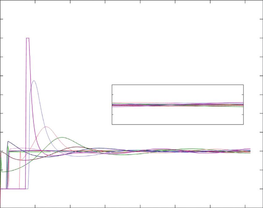
12 Journal of Advanced Transportation

 Table 2: Parameters’ uncertainty.
Index ΔCi (N·s^2/m^2) ΔFi (N)
1 0.5 sin(0.1t) 300 sin(t + 3π/4)
2 0.5 cos(0.2t + π/4) 300 sin(0.9t − 5π/4)
3 0.5 sin(0.3t − 1π/2) 300 sin(0.8t + 3π/2)
4 0.5 sin(0.4t + 3π/4) 300 cos(0.7t − 7π/4)
5 0.5 sin(0.5t − π) 300 sin(0.6t)
6 0.5 cos(0.6t + 5π/4) 300 sin(0.5t − π/4)
7 0.5 cos(0.7t + 3π/2) 300 sin(0.4t − π/2)
8 0.5 cos(0.8t + 7π/4) 300 cos(0.3t + 3π/4)
9 0.5 sin(0.9t) 300 sin(0.2t − π)
10 0.5 sin(t − π/4) 300 cos(0.1t + 5π/4)

 400

 350

 300

 250
 Position (m)

 Chaotic
 200

 150
 Steady
 100

 50

 0
 0 2 4 6 8 10 12 14
 Time (s)

 Vehicle1 Vehicle6
 Vehicle2 Vehicle7
 Vehicle3 Vehicle8
 Vehicle4 Vehicle9
 Vehicle5 Vehicle10
 Figure 7: Position history under proposed controller (41).

 1.5

 0.1
 1
 0

 -0.1
 0.5 12 14
 Gap error (m)

 0

 -0.5

 -1

 -1.5
 0 2 4 6 8 10 12 14
 Time (s)

 Vehicle2 Vehicle7
 Vehicle3 Vehicle8
 Vehicle4 Vehicle9
 Vehicle5 Vehicle10
 Vehicle6
 Figure 8: Gap error history under proposed controller (41).

Journal of Advanced Transportation 13

 30 6. Conclusion
 28
 25 This study proposed a constraint-following control strategy
 25
 for a CAV platoon system to solve the problem of platoon
 20
 22
 12 14
 starting. In these specific processes, the intervehicle dis-
 tances between consecutive CAVs were considered to
 Velocity (m/s)

 construct the control law to guarantee safety and collision
 15
 avoidance. As the U–K approach cannot be directly applied
 to handle inequality constraints, the diffeomorphism
 10 method was adopted to transform the bounded variable into
 an unbounded variable so that the U–K approach could be
 5 employed to render the control law. In addition, parametric
 uncertainties were considered in the designed dynamic
 0 system. Thus, an analytical closed-form control law was
 0 2 4 6 8 10 12 14 proposed for this specific dynamic system.
 Time (s) Comprehensive simulations were performed to validate
 Vehicle1 Vehicle6 the control performance under the conditions of parametric
 Vehicle2 Vehicle7 uncertainty and no parametric uncertainty. The experi-
 Vehicle3 Vehicle8 mental results indicated that the proposed control law
 Vehicle4 Vehicle9 rendered by the U–K approach could meet the performance
 Vehicle5 Vehicle10 requirements of UB and UUB under this specific situation.
 Figure 9: Velocity history under proposed controller (41). Moreover, the intervehicle distance was always confined
 within the specified range, which could guarantee the safety
 of the CAV platoon system. Meanwhile, there are some
 limitations to this study. The study was only concerned
 10
 about the process of platoon starting, however, the stopping
 9 also needs to be considered. Furthermore, the acceleration
 8 and deceleration of the vehicle platoon can be another key
 7 point of platoon control. In the future, we will introduce
 lateral control into this model to solve the lane-changing and
 Acceleration (m/s2)

 6
 3 turning problems related to the CAV platoon. Furthermore,
 5 2.5
 we will establish a more sophisticated vehicle dynamic
 2
 4 1.5 model, including constraints on the spacing error against the
 1
 3 12 14 current position, measurement noise, communication delay,
 2 and mechanical lag, to ensure the safety and stability of the
 CAV platoon system.
 1
 0
 -1
 Data Availability
 0 2 4 6 8 10 12 14
 Time (s) The data used to support the findings of this study are in-
 cluded within the article.
 Vehicle1 Vehicle6
 Vehicle2 Vehicle7
 Vehicle3 Vehicle8 Conflicts of Interest
 Vehicle4 Vehicle9
 Vehicle5 Vehicle10 The authors declare that they have no known competing
Figure 10: Acceleration history under proposed controller (41). financial interests or personal relationships that could have
 influenced the work reported in this paper.

 In contrast to case 2 in section 5.2, fluctuations appear in Acknowledgments
the curves of both the spacing error, velocity, and acceler-
ation, as shown in Figures 8–10, which are obvious in the This work is supported by National Key Research and
partially enlarged figures. These fluctuations are reasonable Development Program of China (No. 2019YFB1600100),
because they are caused by parameter uncertainties, as National Natural Science Foundation of China (No.
mentioned above. It is clear that gap errors tend to converge 61973045), Shaanxi Province Key Development Project (No.
to zero, which is not amplified by the propagation of traffic S2018-YF-ZDGY-0300), Fundamental Research Funds for
flow, although uncertainties exist. It proves that the pro- the Central Universities (No. 300102248403), Joint Labo-
posed controller (41) renders the UB and UUB performance ratory of Internet of Vehicles sponsored by Ministry of
of the constrained uncertain dynamic CAV platoon system. Education and China Mobile (No. 213024170015), and

14 Journal of Advanced Transportation

Application of Basic Research Project for National Ministry Intelligent Transportation Systems Magazine, vol. 12, no. 1,
of Transport (No. 2015319812060). pp. 4–24, 2020.
 [16] B. Xu, S. E. Li, Y. Bian et al., “Distributed conflict-free co-
 operation for multiple connected vehicles at unsignalized
References intersections,” Transportation Research Part C: Emerging
 Technologies, vol. 93, pp. 322–334, 2018.
 [1] D. T. Jia, K. Lu, and J. Wang, “A survey on platoon-based
 [17] S. Tak, S. Kim, and H. Yeo, “A study on the traffic predictive
 vehicular cyber-physical systems,” IEEE Commun. Surv.
 Tutor.vol. 18, no. 1, pp. 263–284, 2015. cruise control strategy with downstream traffic information,”
 [2] S. E. Li, Y. Zheng, K. Li et al., “Dynamical modeling and IEEE Transactions on Intelligent Transportation Systems,
 distributed control of connected and automated vehicles: vol. 17, no. 7, pp. 1932–1943, 2016.
 challenges and opportunities,” IEEE Intelligent Transportation [18] M. Wang, W. Daamen, S. P. Hoogendoorn, and B. van Arem,
 Systems Magazine, vol. 9, no. 3, pp. 46–58, 2017. “Rolling horizon control framework for driver assistance
 [3] E. Moradi-Pari, H. N. Mahjoub, H. Kazemi, Y. P. Fallah, and systems. Part I: mathematical formulation and non-cooper-
 A. Tahmasbi-Sarvestani, “Utilizing model-based communi- ative systems,” Transportation Research Part C: Emerging
 cation and control for cooperative automated vehicle appli- Technologies, vol. 40, pp. 271–289, 2014.
 cations,” IEEE Transactions on Intelligent Vehicles, vol. 2, [19] Z. Yuan, K. He, and Y. Yang, “A roadway safety sustainable
 no. 1, pp. 38–51, 2017. approach: modeling for real-time traffic crash with limited
 [4] B. van Arem, C. J. G. van Driel, and R. Visser, “The impact of data and its reliability verification,” Journal of Advanced
 cooperative adaptive cruise control on traffic-flow charac- Transportation, vol. 2022, Article ID 1570521, 14 pages, 2022.
 teristics,” IEEE Transactions on Intelligent Transportation [20] F. Michaud, P. Lepage, P. Frenette, D. Letourneau, and
 Systems, vol. 7, no. 4, pp. 429–436, 2006. N. Gaubert, “Coordinated maneuvering of automated vehicles
 [5] K. C. Dey, L. Yan, X. Wang et al., “A review of commu- in platoons,” IEEE Transactions on Intelligent Transportation
 nication, driver characteristics, and controls aspects of Systems, vol. 7, no. 4, pp. 437–447, 2006.
 cooperative adaptive cruise control (CACC),” IEEE [21] V. Milanes, S. E. Shladover, J. Spring, C. Nowakowski,
 Transactions on Intelligent Transportation Systems, vol. 17, H. Kawazoe, and M. Nakamura, “Cooperative adaptive cruise
 no. 2, pp. 491–509, 2016. control in real traffic situations,” IEEE Transactions on In-
 [6] M. Wang, W. Daamen, S. P. Hoogendoorn, and B. van Arem, telligent Transportation Systems, vol. 15, no. 1, pp. 296–305,
 “Cooperative car-following control: distributed algorithm and 2014.
 impact on moving jam features,” IEEE Transactions on In- [22] Y. Li, L. Zhang, and H. Zheng, “Nonlane-discipline-based car-
 telligent Transportation Systems, vol. 17, no. 5, pp. 1459–1471, following model for electric vehicles in transportation-cyber-
 2016. physical systems,” IEEE Transactions on Intelligent Trans-
 [7] J. Vanderwelf, S. Shladover, and N. Kourjanskaia, “Modeling portation Systems, vol. 19, no. 1, pp. 38–47, 2017.
 effects of driver control assistance systems on traffic,” Transp. [23] K. Curts, “Temples and turnpikes in “the world of tomorrow”:
 Res. Rec. J. Transp. Res. Board, vol. 1748, pp. 167–174, 2001. religious assemblage and automobility at the 1939 New York
 [8] G. J. L. Naus, R. P. A. Vugts, J. Ploeg, world’s fair,” Journal of the American Academy of Religion,
 M. J. G. van de Molengraft, and M. Steinbuch, “String-stable vol. 83, no. 3, pp. 722–749, 2015.
 cacc design and experimental validation: a frequency-domain [24] J. K. Hedrick, M. Tomizuka, and P. Varaiva, “Control issues in
 approach,” IEEE Transactions on Vehicular Technology, automated highway systems,” IEEE Control Systems Maga-
 vol. 59, no. 9, pp. 4268–4279, 2010. zine, vol. 14, no. 6, pp. 21–32, 1994.
 [9] Q. Xu and R. Sengupta, “Simulation, analysis, and comparison [25] S. S. Stankovic, M. J. Stanojevic, and D. D. Siljak, “Decen-
 of ACC and CACC in highway merging control,” IEEE Intell.
 tralized overlapping control of a platoon of vehicles,” IEEE
 Veh. Symp., 2003.
 Transactions on Control Systems Technology, vol. 8, no. 5,
[10] J. Rios-Torres and A. A. Malikopoulos, “A survey on the
 pp. 816–832, 2000.
 coordination of connected and automated vehicles at inter-
 [26] G. D. Lee and S. W. Kim, “A longitudinal control system for a
 sections and merging at highway on-ramps,” IEEE Transac-
 platoon of vehicles using a fuzzy-sliding mode algorithm,”
 tions on Intelligent Transportation Systems, vol. 18, no. 5,
 pp. 1066–1077, 2017. Mechatronics, vol. 12, no. 1, pp. 97–118, 2002.
[11] Y. Li, K. Li, T. Zheng, X. Hu, H. Feng, and Y. Li, “Evaluating [27] G. Antonelli and S. Chiaverini, “Kinematic control of platoons
 the performance of vehicular platoon control under different of autonomous vehicles,” IEEE Transactions on Robotics,
 network topologies of initial states,” Physica A: Statistical vol. 22, no. 6, pp. 1285–1292, 2006.
 Mechanics and Its Applications, vol. 450, pp. 359–368, 2016. [28] A. Ghasemi, R. Kazemi, and S. Azadi, “Stable decentralized
[12] S. E. Shladover, C. A. Desoer, and J. K. Hedrick, “Automated control of a platoon of vehicles with heterogeneous infor-
 vehicle control developments in the PATH program,” IEEE mation feedback,” IEEE Transactions on Vehicular Technol-
 Transactions on Vehicular Technology, vol. 40, no. 1, ogy, vol. 62, no. 9, pp. 4299–4308, 2013.
 pp. 114–130, 2002. [29] J. I. Ge and G. Orosz, “Optimal control of connected vehicle
[13] S. E. Shladover, “PATH at 20 - history and major milestones,” systems with communication delay and driver reaction time,”
 IEEE Intell. Transp. Syst. Conf., 2006. IEEE Transactions on Intelligent Transportation Systems,
[14] Y. Bian, Y. Zheng, W. Ren, S. E. Li, J. Wang, and K. Li, vol. 18, no. 8, pp. 2056–2070, 2017.
 “Reducing time headway for platooning of connected vehicles [30] N. Chen, M. Wang, T. Alkim, and B. van Arem, “A robust
 via V2V communication,” Transportation Research Part C: longitudinal control strategy of platoons under model un-
 Emerging Technologies, vol. 102, pp. 87–105, 2019. certainties and time delays,” Journal of Advanced Trans-
[15] Z. Wang, Y. Bian, S. E. Shladover, G. Wu, S. E. Li, and portation, vol. 2018, no. 2, pp. 1–13. In press, 2018.
 M. J. Barth, “A survey on cooperative longitudinal motion [31] F. Dong, X. Zhao, J. Han, and Y. H. Chen, “Optimal fuzzy
 control of multiple connected and automated vehicles,” IEEE adaptive control for uncertain flexible joint manipulator based

Journal of Advanced Transportation 15

 on D -operation,” IET Control Theory & Applications, vol. 12,
 no. 9, pp. 1286–1298, 2018.
[32] Z. Yan, M. Wang, and J. Xu, “Global adaptive neural network
 control of underactuated autonomous underwater vehicles
 with parametric modeling uncertainty,” Asian Journal of
 Control, vol. 21, no. 3, pp. 1342–1354, 2018.
[33] G. D. Lee and S. W. Kim, “A longitudinal control system for a
 platoon of vehicles using a fuzzy-sliding mode algorithm,”
 Mechatronics, vol. 12, no. 1, pp. 97–118, 2002.
[34] C. Desjardins and B. Chaib-Draa, “Cooperative adaptive
 cruise control: a reinforcement learning approach,” IEEE
 Transactions on Intelligent Transportation Systems, vol. 12,
 no. 4, pp. 1248–1260, 2011.
[35] E. Kayacan, “Multiobjective $H_{\infty }$ control for string
 stability of cooperative adaptive cruise control systems,” IEEE
 Transactions on Intelligent Vehicles, vol. 2, no. 1, pp. 52–61,
 2017.
[36] S. Wen, G. Guo, and X. Su, “Cooperative control of vehicle
 platoons according to driving visibility status,” Control Theory
 & Applications, vol. 36, no. 7, pp. 1153–1164, 2019.
[37] F. E. Udwadia and R. E. Kalaba, Analytical Dynamics. A New
 Approach, Cambridge University Press, 1996.
[38] C. M. Pappalardo, “A natural absolute coordinate formulation
 for the kinematic and dynamic analysis of rigid multibody
 systems,” Nonlinear Dynamics, vol. 81, no. 4, pp. 1841–1869,
 2015.
[39] X. Liu, S. Zhen, and K. Huang, “A systematic approach for
 designing analytical dynamics and servo control of con-
 strained mechanical systems,” IEEE/CAA Journal of Auto-
 matica Sinica, vol. 002, no. 004, pp. 382–393, 2015.
[40] R. Yu, Y.-H. Chen, H. Zhao, K. Huang, and S. Zhen, “Self-
 adjusting leakage type adaptive robust control design for
 uncertain systems with unknown bound,” Mechanical Systems
 and Signal Processing, vol. 116, pp. 173–193, 2019.
[41] Z. Hu, Z. Yang, J. Huang, and Z. Zhong, “Safety guaranteed
 longitudinal motion control for connected and autonomous
 vehicles in a lane-changing scenario,” IET Intelligent Trans-
 port Systems, vol. 15, no. 2, pp. 344–358, 2021.
[42] H. Yin, Y.-H. Chen, and D. Yu, “Vehicle motion control
 under equality and inequality constraints: a diffeomorphism
 approach,” Nonlinear Dynamics, vol. 95, no. 1, pp. 175–194,
 2019.
[43] F. E. Udwadia and R. E. Kalaba, “On the foundations of
 analytical dynamics,” International Journal of Non-linear
 Mechanics, vol. 37, no. 6, pp. 1079–1090, 2002.
[44] Y.-H. Chen, “Constraint-following servo control design for
 mechanical systems,” Journal of Vibration and Control,
 vol. 15, no. 3, pp. 369–389, 2009.
[45] B. Noble and J. W. Daniel, “Applied linear algebra,” Math-
 ematical Gazette, vol. 72, no. 462, 1988.
[46] Y.-H. Chen and X. Zhang, “Adaptive robust approximate
 constraint-following control for mechanical systems,” Journal
 of the Franklin Institute, vol. 347, no. 1, pp. 69–86, 2010.
[47] R. Zou, J. Sun, and J. Sun, “Leader-following constrained
 distributed adaptive dynamic programming design for mul-
 tiagent systems,” Chinese Automation Congress (CAC),
 pp. 5345–5349, 2019.