Current systematic carbon-cycle observations and the need for implementing a policy-relevant carbon observing system
←
→
Page content transcription
If your browser does not render page correctly, please read the page content below
Biogeosciences, 11, 3547–3602, 2014
www.biogeosciences.net/11/3547/2014/
doi:10.5194/bg-11-3547-2014
© Author(s) 2014. CC Attribution 3.0 License.

Current systematic carbon-cycle observations and the need for
implementing a policy-relevant carbon observing system
P. Ciais1 , A. J. Dolman2 , A. Bombelli3 , R. Duren4 , A. Peregon1 , P. J. Rayner5 , C. Miller4 , N. Gobron6 , G. Kinderman7 ,
G. Marland8 , N. Gruber9 , F. Chevallier1 , R. J. Andres10 , G. Balsamo11 , L. Bopp1 , F.-M. Bréon1 , G. Broquet1 ,
R. Dargaville5 , T. J. Battin12 , A. Borges13 , H. Bovensmann14 , M. Buchwitz14 , J. Butler15 , J. G. Canadell16 ,
R. B. Cook10 , R. DeFries17 , R. Engelen11 , K. R. Gurney18 , C. Heinze19,20,21 , M. Heimann22 , A. Held23 , M. Henry24 ,
B. Law25 , S. Luyssaert1 , J. Miller15,26 , T. Moriyama27 , C. Moulin1 , R. B. Myneni28 , C. Nussli29 , M. Obersteiner7 ,
D. Ojima30 , Y. Pan31 , J.-D. Paris1 , S. L. Piao32 , B. Poulter1 , S. Plummer33 , S. Quegan34 , P. Raymond35 ,
M. Reichstein22 , L. Rivier1 , C. Sabine36 , D. Schimel37 , O. Tarasova38 , R. Valentini3 , R. Wang1 , G. van der Werf2 ,
D. Wickland39 , M. Williams40 , and C. Zehner41
1 Laboratoire   des Sciences du Climat et de l’Environnement, CEA-CNRS-UVSQ, UMR8212, 91191, Gif sur Yvette Cedex,
France
2 VU University Amsterdam, Amsterdam, the Netherlands
3 Euro-Mediterranean Center for Climate Change, CMCC, Division Climate Change Impacts on Agriculture, Forests and

Natural Ecosystems; via Augusto Imperatore 16, 73100 Lecce, Italy
4 Jet Propulsion Laboratory, California Institute of Technology, 4800 Oak Grove Dr, Pasadena, CA 91109, USA
5 School of Earth Sciences, University of Melbourne, Australia
6 Global Environmental Monitoring Unit, Institute for Environment and Sustainability, European Commission Joint Research

Center, Ispra, Italy
7 International Institute for Applied Systems Analysis (IIASA), Schlossplatz 1, Laxenburg, Austria
8 Research Institute for Environment, Energy, and Economics, Appalachian State University, Boone, NC 28608, USA
9 Institute of Biogeochemistry and Pollutant Dynamics and Center for Climate Systems Modeling, ETH Zürich, Zürich,

Switzerland
10 Carbon Dioxide Information Analysis Center, Oak Ridge National Laboratory, Oak Ridge, TN 37831-6290, USA
11 European Centre for Medium-Range Weather Forecast (ECMWF), Shinfield Park, Reading, RG2 9AX, UK
12 Department of Limnology, University of Vienna, A-1090 Vienna, Austria
13 Chemical Oceanography Unit, University of Liège, Institute de Physique (B5), 4000 Liège, Belgium
14 Institute of Environmental Physics (IUP), University of Bremen, Bremen, Germany
15 NOAA Earth System Research Laboratory (ESRL), 325, Broadway, Boulder, CO 80305-3337, USA
16 CSIRO Marine and Atmospheric Research, Canberra, ACT 2601, Australia
17 Department of Geography and Environment, Boston University, Boston, MA 02115, USA
18 School of Life Sciences, School of Sustainability, Arizona State University, Tempe, AZ 85287, USA
19 Geophysical Institute, University of Bergen, Allégaten 70, 5007 Bergen, Norway
20 Bjerknes Centre for Climate Research, Bergen, Norway
21 Uni Bjerknes Centre, Uni Research, Bergen, Norway
22 Max-Planck-Institute for Biogeochemistry, Jena, Germany
23 AusCover Facility, Terrestrial Ecosystem Research Network – TERN, CSIRO, GPO Box 3023, Canberra ACT 2601,

Australia
24 Forestry Department, Food and Agriculture Organization of the United Nations, Via delle Terme di Caracalla, 00153 Rome,

Italy
25 Department of Forest Ecosystems and Society, 321 Richardson Hall, Oregon State University, Corvallis, OR 97331, USA
26 Cooperative Institute for Research in Environmental Sciences, University of Colorado, Boulder, CO 80309, USA
27 Japan Aerospace Exploration Agency (JAXA), Tokyo
28 Department of Earth and Environment, Boston University, Boston, MA 02215, USA

Published by Copernicus Publications on behalf of the European Geosciences Union.
3548                                                               P. Ciais et al.: Current systematic carbon-cycle observations

29 Thales  Alenia Space, Toulouse, France
30 Natural Resource Ecology Laboratory, Campus Mail 1499, Fort Collins, CO 80523-1499, USA
31 US Department of Agriculture Forest Service, Newtown Square, PA 19073, USA
32 Department of Ecology, Peking University, Beijing 100871, China
33 ESA Climate Office, European Space Agency – Harwell, Didcot, Oxfordshire OX11 0QX, UK
34 Centre for Terrestrial Carbon Dynamics, University of Sheffield, Hicks Building, Hounsfield Road, Sheffield S3 7RH, UK
35 Yale School of Forestry and Environmental Studies, 195 Prospect Street, New Haven, CT 06511, USA
36 Pacific Marine Environmental Laboratory, National Oceanic and Atmospheric Administration, Seattle, WA 98115, USA
37 National Ecological Observatory Network, Boulder, CO 80301, USA
38 World Meteorological Organization, 7bis Avenue de la Paix, 1211 Geneva, Switzerland
39 National Aeronautics and Space Administration, Suite 3B74, 300 E Street SW, Washington, DC 20546, USA
40 School of GeoSciences, University of Edinburgh, Edinburgh, EH9 3JN, UK
41 ESA/ESRIN, Earth Observation Applications Engineer, Via Galileo Galilei CP, 64, Frascati Italy

Correspondence to: P. Ciais (philippe.ciais@lsce.ipsl.fr)

Received: 6 May 2013 – Published in Biogeosciences Discuss.: 10 July 2013
Revised: 6 March 2014 – Accepted: 21 March 2014 – Published: 3 July 2014

Abstract. A globally integrated carbon observation and anal-          rently achieved for natural fluxes, although over a small land
ysis system is needed to improve the fundamental under-               area (cities, industrial sites, power plants), as well as the in-
standing of the global carbon cycle, to improve our ability to        clusion of fossil fuel CO2 proxy measurements such as ra-
project future changes, and to verify the effectiveness of poli-      diocarbon in CO2 and carbon-fuel combustion tracers. Addi-
cies aiming to reduce greenhouse gas emissions and increase           tionally, a policy-relevant carbon monitoring system should
carbon sequestration. Building an integrated carbon obser-            also provide mechanisms for reconciling regional top-down
vation system requires transformational advances from the             (atmosphere-based) and bottom-up (surface-based) flux esti-
existing sparse, exploratory framework towards a dense, ro-           mates across the range of spatial and temporal scales rele-
bust, and sustained system in all components: anthropogenic           vant to mitigation policies. In addition, uncertainties for each
emissions, the atmosphere, the ocean, and the terrestrial bio-        observation data-stream should be assessed. The success of
sphere. The paper is addressed to scientists, policymakers,           the system will rely on long-term commitments to monitor-
and funding agencies who need to have a global picture of the         ing, on improved international collaboration to fill gaps in the
current state of the (diverse) carbon observations. We identify       current observations, on sustained efforts to improve access
the current state of carbon observations, and the needs and           to the different data streams and make databases interopera-
notional requirements for a global integrated carbon observa-         ble, and on the calibration of each component of the system
tion system that can be built in the next decade. A key conclu-       to agreed-upon international scales.
sion is the substantial expansion of the ground-based obser-
vation networks required to reach the high spatial resolution
for CO2 and CH4 fluxes, and for carbon stocks for address-
ing policy-relevant objectives, and attributing flux changes          1   Introduction
to underlying processes in each region. In order to establish
                                                                      Global mean atmospheric levels of CO2 have increased by
flux and stock diagnostics over areas such as the southern
                                                                      40 % from about 280 ppm in pre-industrial times (Etheridge
oceans, tropical forests, and the Arctic, in situ observations
                                                                      et al., 1996) to 393.6 ppm by the end of 2012 (WMO,
will have to be complemented with remote-sensing measure-
                                                                      2010; Dlugokencky and Tans, 2012). Levels of CH4 reached
ments. Remote sensing offers the advantage of dense spatial
                                                                      1813 ± 2 ppb in 2011 (WMO, 2012), nearly 2.5 times their
coverage and frequent revisit. A key challenge is to bring
                                                                      pre-industrial value of 700 ppb (Etheridge et al., 1996). The
remote-sensing measurements to a level of long-term consis-
                                                                      increase of CO2 and CH4 is caused by fossil fuel combus-
tency and accuracy so that they can be efficiently combined
                                                                      tion and land use change. The primary anthropogenic CH4
in models to reduce uncertainties, in synergy with ground-
                                                                      emissions are leaks from natural gas extraction and distribu-
based data. Bringing tight observational constraints on fossil
                                                                      tion, the oil industry and coal extraction, livestock and rice
fuel and land use change emissions will be the biggest chal-
                                                                      paddies, landfills and human-caused biomass burning (Den-
lenge for deployment of a policy-relevant integrated carbon
                                                                      man et al., 2007). Natural emissions of CH4 are dominated
observation system. This will require in situ and remotely
                                                                      by wetlands and lakes, with smaller contributions from geo-
sensed data at much higher resolution and density than cur-
                                                                      logical natural venting, wildfires, and termites.

Biogeosciences, 11, 3547–3602, 2014                                                        www.biogeosciences.net/11/3547/2014/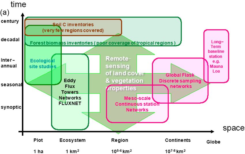
P. Ciais et al.: Current systematic carbon-cycle observations                                                               3549

   Fossil fuel emissions increased at a rate of 3.1 % per year     design details of the monitoring system and their costs. Issues
over the last decade (Le Quéré et al., 2013). Rates of land        of economies of scale, i.e. single country or even projects
use change CO2 emissions have slightly declined in the past        versus a global system, and economies of scope generated
decade (Friedlingstein et al., 2010).                              by constellations of monitoring systems are crucial determi-
   Emission reduction programs are developed in support            nants of choice (Böttcher et al., 2009).
of international agreements, such as United Nations Frame-            Natural fluxes need to be measured in order to un-
work Convention on Climate Change (UNFCCC). Yet, an-               derstand the mechanisms controlling atmospheric concen-
thropogenic emissions of CO2 and CH4 estimated from in-            trations. Globally, natural land and ocean sinks have ab-
ventories cannot be validated by independent observations.         sorbed 56 ± 6 % of CO2 from anthropogenic emissions since
The ability of nations, provinces, and local municipalities to     1959 (Ciais et al., 2013). Regionally, ocean gyres and sub-
implement policies that reduce emissions or create sinks of        continental fluxes can be either sources or sinks of CO2 . At
CO2 and CH4 (de Richter and Caillol, 2011; Kucharczyk,             synoptic scales, the uncertainty of natural fluxes is as large
2011; Stolaroff et al., 2012) will partly depend upon their        as their mean value (NRC, 2010; Denman et al., 2007). The
ability to measure progress, and evaluate effectiveness of na-     global growth rate of CO2 exhibits interannual fluctuations
tional and sub-national actions. Uncertainties in inventories      that reflect climate-induced changes in terrestrial (mainly
need to be dramatically reduced to support effective poli-         tropical) ecosystem fluxes (Le Quèrè et al., 2009; Alden
cies. To date, efforts to monitor and report emissions of CO2      et al., 2010). Regionally, interannual variability of ocean
and CH4 have been based mostly on limited large-scale, sub-        fluxes can also be significant, for example, in the tropical
sampled land use observations, self-reported data on land and      Pacific and the North Atlantic (Watson et al., 2009; Feely
energy use, and extrapolated emission factor measurements.         et al., 1999). This interannual variability of fluxes requires
These data have uncertainties that limit their ability to sup-     longer time series of atmospheric measurements to detect
port greenhouse management strategies (e.g. Schulze et al.,        slow changes in CO2 and CH4 emissions and sinks. The cur-
2009). For instance, even in developed nations where uncer-        rent state of research-based observations can neither confi-
tainties in annual fossil CO2 emissions are ∼ 5 % (Andres          dently account for regional fluxes that control the CO2 and
et al., 2012), the total uncertainty associated with those esti-   CH4 average growth rate nor their interannual changes.
mates over multiple years exceed the magnitude of the trends          Making accurate future projections requires a quantifica-
defined as the target of emission reduction policies (e.g. the     tion of the history of ecosystems’ carbon pools and their
Kyoto Protocol target set by EU15 members of a collective          likely changes in response to business as usual (BAU) human
reduction of 8 % of during 2008–2012 of their emissions be-        behavior and climate policy interventions. Further, changes
low the 1990 level; EEA, 2009, p. 9).                              in the role of the ocean as a global sink for atmospheric CO2
   Improved scientific understanding of the carbon cycle is        can have huge consequences for greenhouse gas (GHG) man-
a critical foundation to providing policy-relevant informa-        agement, so that monitoring ocean fluxes, and their changes
tion regarding climate change mitigation and adaptation in         in response to climate, is also a key for making accurate fu-
three ways: (1) by providing understanding of the processes        ture projections.
controlling the carbon cycle to estimate ex ante the likely           The RECCAP (REgional Carbon Cycle Assessment and
impacts of implementation the greenhouse gas (GHG) man-            Processes) project (Canadell et al., 2011) attempts to recon-
agement strategies, (2) by informing the construction of an        cile bottom-up and top-down flux estimates. However, it also
accurate baseline of GHG fluxes and carbon stocks against          exposed large data gaps and uncertainties that prevent cur-
which climate policies can be evaluated, and (3) by monitor-       rent systems from delivering information to support climate
ing the variability and long-term trends of GHG fluxes over        policies or to resolve carbon–climate feedbacks. Unlike other
each region ex post assessment of the efficacy of mitigation       emission reduction efforts, such as the 1987 Montreal proto-
policies (most of which span decades).                             col, reducing CO2 and CH4 emissions will have to involve
   Anthropogenic emissions would need to be measured not           many economic sectors of society. It will also require many
only for global annual totals but also for their spatiotemporal    decades of sustained effort (Pacala and Socolow, 2004), and
distribution. Timely delivery of such information is critical      sufficient spatial resolution to be able to monitor and man-
for policy. For example, Reduced Emissions from Deforesta-         age impacts resulting from specific governmental policies.
tion and Degradation (UN-REDD, 2008) projects under the            Large-scale, non-carbon emission reductions in the past have
UNFCCC have been held back due to technical and institu-           all required some approach to monitoring and verification
tional barriers, with one analysis suggesting that only 3 out of   to ensure that the desired outcomes are achieved (e.g. mea-
99 tropical countries have the capacity to produce good qual-      surements of pH in lakes and rain for sulfur emission reduc-
ity forest area change and forest inventories (Herold, 2009).      tion; measurements of ozone and ozone-depleting gases for
As an example, Panama’s deforestation would need to in-            stratospheric ozone recovery; and measurements of ozone,
crease by 50 % in absolute value before it could be detected       reactive gases and particulate matter for regional air quality
by the current national capability (Pelletier et al., 2011). The   improvement). However, the global scale of the problem, the
scope of climate policies will have a significant impact on the    natural and anthropogenic components, the many sources of

www.biogeosciences.net/11/3547/2014/                                                      Biogeosciences, 11, 3547–3602, 2014
3550                                                              P. Ciais et al.: Current systematic carbon-cycle observations

carbon and other GHGs, and links to many sectors of the                – What are the magnitudes, distribution, variability, and
economy make independent monitoring and verification of                  trends of regional natural CO2 and CH4 fluxes, and what
the effectiveness of GHG management strategies a necessary               does this information tell us about the underlying natu-
albeit daunting task. Thus, the ability to measure GHG fluxes            ral and human induced mechanisms in each region?
and carbon pools at high spatial and temporal resolution is
fundamental to making this task tractable.                             – What and were are the magnitudes, distribution, vari-
   Last, it is possible that continued climate change driven             ability, and trends of regional carbon stocks in natural
by GHG emissions could cause CO2 and CH4 losses from                     and managed ecosystems?
natural ecosystems, acting as positive feedbacks on climate
                                                                       – How are CO2 and CH4 sources and sinks likely to be-
change. These feedbacks could become particularly intense.
                                                                         have in the future under higher atmospheric CO2 con-
A detailed spatially resolved observing system with the ca-
                                                                         centrations and altered patterns of atmospheric com-
pacity of accurate monitoring of trends or abnormal vari-
                                                                         position (nitrogen deposition, elevated ozone), climate,
ability in CO2 or CH4 fluxes, and changes in carbon stor-
                                                                         land vegetation, and ocean circulation as well as from
age, could be used in an “early warning” mode to detect
                                                                         human appropriation of terrestrial and marine resources
“hotspots” and to guide adaptation planning. Observations
                                                                         impacting the carbon cycle?
with particular emphasis over sensitive regions of the global
carbon cycle (permafrost, tropical forests, North Atlantic and         – How soon might positive/negative feedbacks that may
southern oceans where deep water formation occurs) are thus              enhance/reduce natural CO2 and CH4 emissions, re-
essential to improve our knowledge of carbon-cycle feed-                 duce/enhance sinks, possibly associated with thresh-
backs.                                                                   olds, come into play over different sensitive regions, and
   This paper describes the current state of research-based              how could these feedbacks be detected and quantified
carbon observations (Sect. 3) and a strategy for a globally in-          by observations?
tegrated carbon-cycle monitoring system (Sect. 4) designed
to make possible the estimation of the distribution of CO2           This study builds on the Integrated Global Observing
and CH4 fluxes with sufficient accuracy to assess natural pro-       System-Partnership (IGOS-P) Carbon Theme Team report
cesses and human intervention. In addition, the monitoring           (Ciais et al., 2004) and on a more recent report prepared for
system will be able to assess the spatial and temporal distri-       the Group on Earth Observations (GEO) (Ciais et al., 2010),
bution of fossil fuel and land use related emissions to support      and the US National Research Council report on quantify-
the verification of emission reduction at national and regional      ing and verifying greenhouse gas emissions (NRC, 2010).
scales, while linking them back to global emission quantities        The carbon observing system outlined in this study will ul-
and growth in atmospheric CO2 and CH4 .                              timately need to address all carbon greenhouse gases and
                                                                     N2 O, but we are focusing on a “carbon system” for CO2 and
                                                                     CH4 because these two gases represent the highest share of
2    Framework for the carbon monitoring system                      increased radiative forcing (Hofmann et al., 2006). An in-
                                                                     tegrated observing system with the capacity to enable esti-
Although research priorities for carbon-cycle science are es-        mations of N2 O fluxes is not described here, but could be
tablished, climate policies including detailed provisions of         established following similar principles and technology as
emission reduction treaties, national legislation, and volun-        for CH4 (Hirsch et al., 2006; NRC, 2010; Phillips et al.,
tary programs are only partially defined and will continue to        2007; Corazza et al., 2011). National and sovereign circum-
evolve over the coming decades. This complicates the for-            stances will naturally dictate the complexity and type of na-
mulation of requirements for an integrated carbon monitor-           tional monitoring systems that individual countries might
ing system, and the assessment of relative strengths of dif-         agree to establish for reporting emissions to the United Na-
ferent observational approaches and model-data integration           tions Framework Convention on Climate Change (UNFCCC)
schemes. In order to provide a necessary context for the pro-        and for avoiding greenhouse gas losses from ecosystems. Or-
posed strategy, we establish in this study a framework for a         ganizations like the Group on Earth Observation (GEO), the
carbon monitoring system based on the following questions:           World Meteorological Organization (WMO), and the Food
                                                                     and Agriculture Organization (FAO) can play an impartial,
    – What are and were the magnitudes, distribution, vari-          international, scientific role here in coordinating global ob-
      ability and trends of anthropogenic CO2 and CH4 emis-          servations and facilitating unencumbered access by all coun-
      sions, including their attribution to relevant sectors?        tries to relevant data, information, tools, and methodologies.
                                                                     Existing institutions could also be improved to fulfill such a
    – How effective will national, regional, and city- and           role (Le Quéré et al., 2010). Policy frameworks on how to
      project-scale policy interventions be in reducing green-       manage the biospheric carbon cycle for GHG mitigation are
      house gas emissions and/or increasing carbon seques-           still in a primordial state. In this paper we do not foresee yet
      tration?                                                       specific climate policy implementation mechanisms such as

Biogeosciences, 11, 3547–3602, 2014                                                       www.biogeosciences.net/11/3547/2014/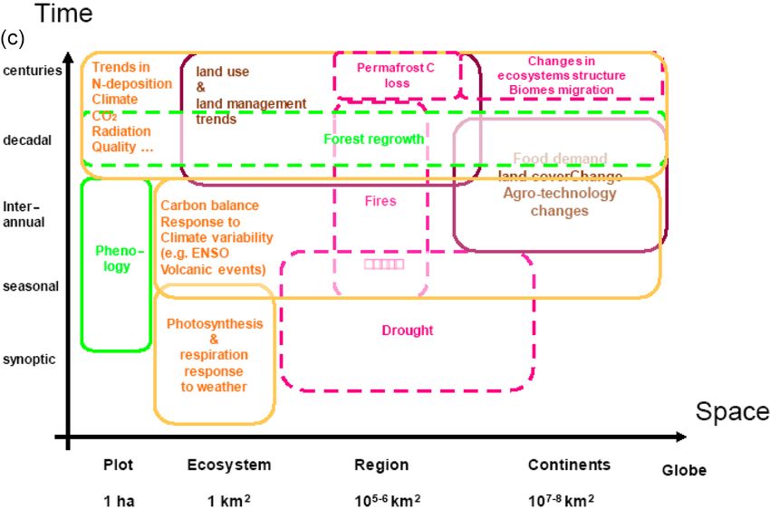
P. Ciais et al.: Current systematic carbon-cycle observations 3551
performance base payments or activity-based mechanisms, Because fossil CO2 emissions are currently prescribed as
which would obviously drive the design of specific observa- boundary conditions of atmospheric inversion models, they
tional components. must be measured at the same space/time resolution as the
numerical simulation of transport. This implies the objective
of characterizing emissions at the scales of 1 km each hour,
3 Current carbon-cycle observations including geo-referenced information on large point sources,
as appropriate to meso-scale inversion models (Broquet et
3.1 State of the art
al., 2011; Lauvaux et al., 2012). This is why over some re-
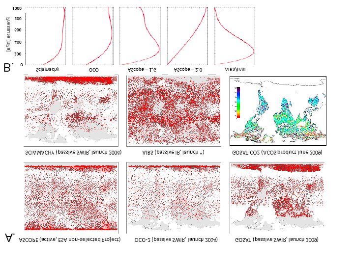
The spatial and temporal scales of coverage of current ter- gions, like North America (Gurney et al., 2009; Pétron et
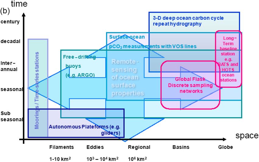
restrial and oceanic observation assets are depicted in Fig. 1a al., 2008), Europe (Pregger et al., 2007) and Southeast Asia
and b, along with processes impacting the carbon balance of (Ohara et al., 2007; Wang et al., 2013) pilot fossil CO2 emis-
ecosystems and air–sea fluxes (Fig. 1c and d). There is (to sions data products exist at higher spatial resolution, parti-
our knowledge) no global data-product providing the global tioned between economic sectors and temporal profiles. Usu-
spatial distribution of fossil fuel CO2 and CH4 emissions, ally, no error structure is associated with fossil fuel emission
or of land use change CO2 emissions, including detailed data products, although Rayner et al. (2010) described an al-
(e.g. hourly) temporal profiles. One can see from Fig. 1 that gorithm to generate one.
the mechanisms controlling carbon fluxes in the long term Three examples of global and regional fossil emission geo-
will evolve during the next decades, and are not well sam- referenced data-products are shown in Fig. 2. The first one
pled by current observing systems. is the above-listed EDGAR (www.edgar.jrc.ec.europa.eu) at
Over the past ten years, carbon measurements have been 10 km spatial resolution, with no temporal profile. The sec-
collected through various programs and projects. Spatial cov- ond is the VULCAN detailed US fossil fuel emission inven-
erage has either stagnated (many regions still un-sampled) tory here given hourly at 10 km resolution, obtained from
or moderately increased through the establishment of in situ local/regional air pollution monitoring data complemented
monitoring stations (e.g. ICOS – Integrated Carbon Ob- with census, traffic, and digital road data sets (vulcan.project.
servation System in Europe; http://www.icos-infrastructure. asu.edu/index.php; Gurney et al., 2009). The third one is a
eu), and better access and continuity to key space-based ∼ 1 km spatial resolution map of emissions, with temporal
remote-sensing platforms. Implementation has largely re- allocation, covering Europe (here we show France only) ob-
mained through research programs, rather than being de- tained by disaggregating national emission totals using var-
signed with an operational integrated monitoring system in ious activity data for industry, road traffic, and urban use
mind. There is attrition (e.g. closure of Canadian Carbon Pro- (www.carboeurope.ier.uni-stuttgart.de/).
gram flux sites, risks for the National Oceanic and Atmo- Global annual fossil fuel CO2 emission values are esti-
spheric Administration – Earth System Research Laboratory mated to have an uncertainty in the range 3–10 % (1-sigma;
(NOAA-ESRL) flask sampling network (Houweling et al., most of the uncertainty can be considered as bias, e.g. from
2012) and some atmospheric monitoring stations in Europe). the use of different statistical data), depending on whether
Another obvious gap is the lack of global biomass monitor- or not the data of three primary fuels (gas, oil, and coal) are
ing capacity. independent of each other (Marland et al., 2009). Estimates
for individual countries can have much larger uncertainty,
3.2 Fossil fuel emissions up to several tens of %, especially for developing countries
(NRC, 2010). A comparison between the CDIAC and the
Current data sets of fossil fuel CO2 emissions averaged Dutch National Institute for Public Health and the Environ-
by country, sector and year are maintained by the Inter- ment (RIVM) of fossil CO2 emissions at the country level
national Energy Agency (IEA, 2012) (http://www.iea.org/ showed that the largest percentage emission differences are
co2highlights/co2highlights.pdf), the Carbon Dioxide Infor- for some developing countries (Marland et al., 1999) but that
mation Analysis Center (CDIAC) (Boden et al., 2012) based the largest absolute differences remains for high-emission
on the United Nations Statistics Division (UNSO) energy countries with the best statistical system. The two estimates
data set, and Emission Database for Global Atmospheric for the USA, for example, differed by only 0.9 %, but in abso-
Research – EDGAR4.2 (a product of the Joint Research lute terms this difference was larger than the total emissions
Center of the European Commission (JRC) together with from 147 of the 195 countries considered. Better data on fos-
the Netherlands Environmental Assessment Agency (PBL) sil fuel consumption and the human activities that are most
(EDGAR4-database, 2009) based on IEA energy data set. related to fuel-consumption will be essential in establish-
Emission maps exist over the globe from different data prod- ing priorities, evaluating success, and confirming agreements
ucts (Andres et al., 1996) with limited temporal information (NRC, 2010). Potential approaches for this are addressed in
(e.g. monthly in Andres et al., 2011). Sect. 4.
www.biogeosciences.net/11/3547/2014/ Biogeosciences, 11, 3547–3602, 2014
3552                                                                P. Ciais et al.: Current systematic carbon-cycle observations

Figure 1. Example of the range of diverse carbon observations that need to be integrated across time and space scales. (A) Terrestrial flux
perspective, (B) marine fluxes perspective, (C) terrestrial carbon-cycle processes action on the same space–time diagram, and (D) marine
carbon processes.

Biogeosciences, 11, 3547–3602, 2014                                                           www.biogeosciences.net/11/3547/2014/
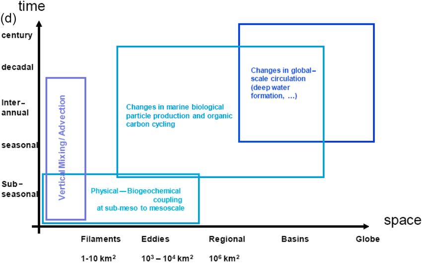
P. Ciais et al.: Current systematic carbon-cycle observations                                 3553

Figure 1. Continued.

www.biogeosciences.net/11/3547/2014/                            Biogeosciences, 11, 3547–3602, 2014
3554 P. Ciais et al.: Current systematic carbon-cycle observations
90°N mospheric measurements (Schmitgen et al., 2004; Zupanski
et al., 2007; Lauvaux et al., 2012; Göckede et al., 2010; Bro-
45°N quet et al., 2011; Lauvaux et al., 2009). However, the current
sparseness of the ground-based network of atmospheric sta-
0° tions cannot constrain the patterns of CO2 sources and sinks
at the scale of nations, states/provinces, or cities (Hunger-
45°S shoefer et al., 2010; Chevallier et al., 2010), although some
A Unit: Mg C/km2/yr country-level estimates have been derived for CH4 in Europe
90°S 0 0.01 0.1 1 10 30 50 100 200 400 10000 (Bergamaschi et al., 2010).
180°W 120°W 60°W 0° 60°E 120°E 180°E The current atmospheric concentration surface network
contains 200 flask and in situ continuous measurement sta-
49.2°N 51.1°N
tions. Its density is higher in North America, Europe and
Japan (Fig. 3). Data from stations reporting to the World
Meteorological Organization (WMO) Global Atmosphere
Watch (GAW) program can be found at the World Data Cen-
ter for Greenhouse Gases (WDCGG; www.gaw.kishou.go.jp/
B C wdcgg/) (WMO, 2009). Atmospheric CO2 observations over
24.8°N 42.1°N
125.2°W 66.4°W 4.9°W 8.3°E the ocean are made on ships and moorings at a few loca-
Emission, kg C/m2/yr Emission, kg C/m2/yr
tions. The current situation is that no accuracy information is
0.01 0.03 0.05 0.1 1 5 0.01 0.03 0.05 0.1 1 5
1
reported with atmospheric measurements from each station.
2 Figure 2. Fossil fuel emission maps obtained from current invento- The tropics and Southern Hemisphere are under-sampled.
3 Fig.
ries.2. Fossil fuel emission
(A) Annual maps obtained
emission mapfrom
forcurrent
the inventories. A. Annual
year of 2010 fromemission
EDGAR map for Aircraft vertical profile measurements of CO2 and CH4
4 the year of 2010
(release from EDGAR
version-4.2 (release version-4.2
FT2010). FT2010). The is
The resolution resolution
10 km. is 10 B. Fossil
km.Fossil
(B) are particularly important for the independent evaluation of
5 fuel
fuelemission map ofmap
emission the US
offorthe
the US
year of
for2002
thewith temporal
year variability
of 2002 withobtained from air
temporal vertical mixing in atmospheric transport models (Stephens
6 pollution data, traffic
variability obtainedand other
fromindustrial activity data data,
air pollution from the VULCAN
traffic, project
and other(version
indus-2.2).
et al., 2007) as well as elements of remote-sensing val-
7 The
trialresolution
activity is the one from
data of eachthe
activity. C. Map of fossil
VULCAN projectfuel emissions
(versionfor2.2).
the year
Theof 2007
res-at
8 10 km – hourly
idation. Regular vertical-profile sites using dedicated air-
olution is theforone
France, obtained
of each by disaggregation
activity. (C) Map of of
national emission
fossil statistics using
fuel emissions
9 activity
craft exist at about 30 sites around the world without long-
for thedata and of
year emission
2007factors
at 10forkmeach source of for
– hourly emission from IER,
France, Stuttgartby
obtained (the IER
dis-
10 product has a European
aggregation coverage). The
of national same color
emission scale is applied
statistics using
data and for (B) and (C).
activity term funding (Fig. 3a), mostly in North America (Crevoisier
11 emission factors for each source of emission from IER, Stuttgart et al., 2010), and operated by National Oceanic and At-
(the IER product has a European coverage). The same color scale is mospheric Administration – Global Monitoring Division
applied for (B) and (C). 106
(NOAA-GMD) (www.esrl.noaa.gov/gmd/ccgg/aircraft/) or
intensive research projects (e.g. California Nexus (CalNex),
Wennberg et al., 2012). Research projects established regular
3.3 Atmospheric domain aircraft measurements in Siberia (Levin et al., 2002; Maksyu-
tov et al., 2003; Paris et al., 2010) and recently over the Ama-
3.3.1 Surface networks of in situ measurement stations, zon (Gatti et al., 2010; Miller et al., 2007).
and flask air-sampling stations Instrumented commercial aircraft programs (Machida et
al., 2008; Matsueda et al., 2008) Comprehensive Observa-
Measurements of atmospheric CO2 and CH4 complement lo- tion Network for trace gases by Airliner (CONTRAIL) (http:
cal (i.e. ∼ 1 m2 to ∼ 1 km2 ) observations of fluxes and pools //www.cger.nies.go.jp/contrai) and civil aircraft for the reg-
at the ocean and land surface to verify measurements of car- ular investigation of the atmosphere based on an instrument
bon stock changes and process-level variables at large spa- container (CARIBIC) (www.caribic-atmospheric.com/) have
tial and temporal scales. The integrative properties of at- been collected both continuous and flask CO2 , CH4 , and
mospheric mixing mean that atmospheric concentrations of other gases measurements of both vertical profiles during as-
CO2 and CH4 reflect flux processes over large spatial scales. cent and descent and horizontal transects at the cruising alti-
While lacking the process specificity of small-scale ocean or tude of the aircraft (Fig. 3c).
land reservoirs, atmospheric measurements implicitly incor- In 2012, a Corporate Venture announced its intention to
porate all sources and sinks (known and unknown) of a given build up to ∼ 100 CO2 in situ atmospheric continuous sites
gas. (Earth Networks; http://www.earthnetworks.com). The Na-
Inversion of fluxes from concentrations to derive surface tional Ecological Observatory Network (NEON) in the US
fluxes using transport models has already proved capable of (http://www.neoninc.org/) will operate 60 sites with high-
providing global-scale, and in some instances continental- quality calibrated in situ CO2 observations, and the Eu-
scale, information on fluxes with uncertainties. Some pilot ropean Infrastructure ICOS (http://www.icos-infrastructure.
studies have applied atmospheric inversion models at a finer eu/) will develop about 35 stations in its first phase. While
scale down to ∼ 1 km, constrained by regionally denser at- these efforts will likely increase observation density in North
Biogeosciences, 11, 3547–3602, 2014 www.biogeosciences.net/11/3547/2014/
P. Ciais et al.: Current systematic carbon-cycle observations 3555
3.3.2 Satellite observations of column CO2 and CH4
mixing ratio
Satellite remote sensing of column CO2 and CH4 mixing ra-
tio with global coverage offers options to complete atmo-
spheric observations over regions with too low surface net-
A B work density (Fig. 4). Progress has been achieved in the
1 exploitation of existing multipurpose sensors and towards
2 Dedicated aircraft profiles (pink) and passenger aircraft (blue) the design of dedicated GHG satellite instruments. Accu-
rate quantification of regional-scale GHG surface fluxes is
however challenging, as demanding relative accuracy re-
quirements have to be met, especially for CO2 (Bréon and
Ciais, 2009). The initial version of the GOSAT (Greenhouse
gases Observing SATellite) operational total column dry air
mole fraction XCO2 and XCH4 retrieval algorithm suffered
C from significant biases and large scatter when compared
3 to ground-based Total Carbon Column Observing Network
4 (TCCON) observations, but this has been improved (Yoshida
Figure 3. (A) Global network of CO surface stations with flask
Fig. 3. A. Global network of CO2 surface stations with2flask sampling (red symbols) and
5
sampling (red symbols) and continuous measurement sites (blue
et al., 2013). Consequently, some preliminary CO2 flux es-
6 continuous measurement sites (blue symbols). The data from these sites and from additional timates have been produced (Maksyutov et al., 2013; Basu
7
symbols). The data from these sites and from additional stations
stations can be found at WMO GAW World Data Center for Greenhouse Gases
can be found at WMO GAW World Data Center for Greenhouse et al., 2013). For methane the situation is better than for
8 (http://ds.data.jma.go.jp/gmd/wdcgg/). B. Locations of the Total Column Carbon Observing
Gases (http://ds.data.jma.go.jp/gmd/wdcgg/). (B) Locations of the CO2, but satellites still need to be used with in situ data to
9 Network by year 2012. These stations are essential for satellite column CO 2, CH4 measurement
10
Total Column Carbon Observing Network by year 2012. These sta-
validation. C. Location of vertical profile sites, where GHG mixing ratios are measured by
infer methane surface fluxes, as shown by Bergamaschi et
11
tions are essential for satellite column CO and CH4 passenger
dedicated aircraft on a typical monthly basis (pink symbol), 2and location of
measurement al. (2009) using XCH4 retrievals obtained from the SCanning
12
validation. (C) Location of vertical profile sites,
instrumented aircraft program flights CONTRAIL and CARIBIC (blue lines).
where GHG mix- Imaging Absorption spectroMeter for Atmospheric CHartog-
ing ratios are measured by dedicated aircraft on a typical monthly raphY (SCIAMACHY) together with flask measurements.
13
basis (pink symbol), and location of passenger instrumented aircraft Existing/near-launch instruments for column GHG mix-
14
program flights CONTRAIL and CARIBIC (blue lines). ing ratios make measurements either in the thermal infrared
15
16
spectral domain, with peak sensitivity in the middle tro-
posphere: Atmospheric Infrared Sounder (AIRS), Infrared
17 America and Europe, the commercialization of environmen-
Atmospheric Sounding Interferometer (IASI), and Thermal
tal monitoring is a new concept that has to be evaluated over107
Emission Spectrometer (TES), Greenhouse gases Observing
an extended period. But large gaps in atmospheric observa-
SATellite (GOSAT), or in the solar infrared domain: SCIA-
tions still exist in northern Eurasia, Asia, Africa, and South
MACHY (2002–2012), Greenhouse Gas Observing Satellite
America because very few research sites exist.
(GOSAT), Orbiting Carbon Observatory-2 (OCO-2), with a
A key element of surface and aircraft in situ atmospheric
more uniform sensitivity to CO2 and CH4 throughout the
observation programs is their unique capability to closely
atmospheric column, including the boundary layer (Fig. 4).
link all observations to a single CO2 and CH4 dry air mole
The thermal infrared sounders are not well adapted to infer-
fraction scale defined by the WMO. However, while most re-
ring surface fluxes as illustrated by Chevallier et al. (2009a),
search groups make a concerted effort to calibrate their mea-
in contrast to near-infrared sounders. Despite this drawback,
surements to the WMO scale very frequently are obtained
several groups have used thermal infrared sounders to pro-
via regular analysis of standard gases. The current situation
vide information on column variability (Crevoisier et al.,
is that there is no regulatory quality-assurance system en-
2004; Chahine et al., 2008; Xiong et al., 2008).
suring the monitoring of the compatibility and traceability
The precision and accuracy of space-based remotely
of measurements at each site to the WMO scale. Ongoing
sensed GHG column concentration products vary with in-
voluntary-based comparisons of both standard gases and en-
strument and sampling strategy. Unlike in situ sensors, the
vironmental air samples provide means to assess the quality
concentrations of gases in the measurement path cannot be
of linkages between given sites or laboratory measurements
controlled. Thus the direct calibration to the WMO mole
to the international scales. If the effort to link measurements
fraction scale cannot be established for space-based GHG
from multiple networks is to succeed, it is of the utmost im-
column concentration. An indirect data evaluation can be
portance that observed CO2 and CH4 concentration differ-
made using TCCON total column measurement network
ences can be attributed unequivocally to physical processes
data, which themselves can be evaluated against WMO mole
(and not to differences in calibration).
fraction scale airborne in situ vertical profiles (Wunch et al.,
2010, 2011a). For middle-tropospheric CO2 column abun-
dances from infrared sounders, precision estimates of 1 ppm
www.biogeosciences.net/11/3547/2014/ Biogeosciences, 11, 3547–3602, 20143556 P. Ciais et al.: Current systematic carbon-cycle observations
1
2
Figure 4. (A) Spatial sampling of the atmosphere by different satellite instruments ASCOPE (an active mission with a lidar not selected by
ESA); OCO-2, GOSAT, and SCIAMACHY with measurements of reflected sunlight in near infrared, and their vertical weighting functions;
3 Fig.
AIRS 4. A.
(or IASI) Spatial
with sampling
measurements fromof the atmosphere
emission in the mid-IR bydomain,
different satellite
(B) actual instruments
column ASCOPE
XCO2 measurements (anGOSAT XCO2
from
4 active mission with a LIDAR not selected by ESA); OCO-2, GOSAT and SCIAMACHY with
(ACOS product, 2009). X axis units is the dimensionless weight in each atmospheric layer.
5 measurements of reflected sunlight in near infra-red, and their vertical weighting functions; AIRS
on 2◦ spatial and bi-weekly temporal scale for AIRS (Maddy ases (e.g. aerosol concentrations or albedo) are likely to be
6 al., (or
et IASI)
2008), with
2 ppm measurements
precision from
on 5◦ spatial and emission in the mid-IR
monthly tem- coherentdomain,
over spaceB. and
Actual
time,column XCO
requiring 2
significant care to
poral scale for IASI (Crevoisier et al., 2009a), and 10 ppm avoid interpreting them as geophysical signals. The launch
7 measurements
single fromfor
sounding precisions GOSAT XCO2 (ACOS
TES (Kulawik product,of2009).
et al., 2010) GOSATXand axistheunits is the
planned dimensionless
launch of OCO-2 in 2014 have
8 weight in each atmospheric layer.
are reported. For XCO 2 from solar backscatter measure- raised expectations for CO 2 inversions because these two
ments, precision estimates for single soundings of 3 ppm dry instruments are the first ones to have been specifically de-
9 mole fraction for SCIAMACHY (Reuter et al., 2011),
air signed for the detection of atmospheric CO2 (see for exam-
and 2 ppm for GOSAT (Yoshida et al., 2013) are reported. ple, Chevallier et al., 2009b, their Fig. 4). In addition, the
10
Spatially and temporally aggregation of SCIAMACHY and methods are under development to account for large-scale bi-
GOSAT data further improve the precision, if errors are ases using TCCON data (Wunch et al., 2011b).
11
mainly random, depending on cloud cover and spatial sam- For current mid-to-upper tropospheric concentrations of
pling. Future missions like OCO-2 and Carbon Monitoring methane (CH4 ) from thermal infrared sounders like IASI,
12
Satellite (CarbonSat) target aggregated precisions of 1 ppm reported precision estimates are in the range of 17–35 ppb
and better. on 5◦ spatial and monthly temporal scale (Crevoisier et al.,
13 Biases of XCO2 at various space and timescales have ham- 2009b). For XCH4 , reported precision estimates for indi-
pered inversion studies from these products (Chevallier et al., vidual soundings are about 17–35 ppb for SCIAMACHY
14
2005) despite the progress (Maksyutov et al., 2013). These (Frankenberg et al., 2006) and 12.5 ppb for GOSAT (Yoshida
biases can be caused by uncertainties in the spectroscopy et al., 2013). Spatially and temporally aggregated precisions
15
used in the retrieval model, or aliasing with other atmo- of SCIAMACHY and GOSAT can reach the 10 ppb level
spheric signals like aerosols (Houweling et al., 2005). Bi- (and even below for GOSAT) depending on cloud cover
108
Biogeosciences, 11, 3547–3602, 2014 www.biogeosciences.net/11/3547/2014/P. Ciais et al.: Current systematic carbon-cycle observations 3557
and spatial sampling. Future missions like CarbonSat tar- plete space qualifications. One example of such a system
get aggregated measurement precisions of 5 ppb. As shown is the NASA Carbon in Arctic Reservoirs Vulnerability Ex-
by Bergamaschi et al. (2009), biases in satellite XCH4 re- periment (CARVE) which provides aircraft remote sensing
trievals can be (arbitrarily) corrected when calculating fluxes of XCO2 and XCH4 , backed by a comprehensive suite of
by anchoring the inversion with surface in situ station mea- flasks and in situ sensors, and a microwave soil-moisture
surements. More development is required in the rigorous sta- sensor. Another example is the Methane Airborne Mapper
tistical weighting of sparse, but high-accuracy in situ ob- (MAMAP) that includes a grating spectrometer offering re-
servations with much more numerous, but potentially noisy mote sensing of CO2 and CH4 column averaged mixing
and biased satellite observations. This opens the possibility ratios (Gerilowski et al., 2011). Data from MAMAP gath-
of a decadal monitoring of global CH4 fluxes from SCIA- ered during several campaigns and its analysis using inverse
MACHY and GOSAT, in orbit since March 2002 and January plume modeling demonstrated that single CO2 and CH4
2009, respectively, combined with surface in situ network. point source emissions can be detected and quantified in-
The critical potential contribution of satellite XCO2 and dependently using remote-sensing data (Krings et al., 2011,
XCH4 observations to improving atmospheric flux inver- 2013). In addition, light detection and ranging (lidar) air-
sions is clearly their ability to increase the density of ob- borne measurements of CO2 and CH4 have been performed,
servations. Well-calibrated and precise satellite observations the latter in preparation of the Methane Remote Lidar (MER-
should offer the potential to reduce some of the uncertain- LIN) mission (Fig. 7).
ties associated with sparse sampling. However current assets
are far from perfect in terms of spatial coverage, spatial res- 3.3.4 Surface network of remote-sensing measurement
olution, near-surface sensitivity, and temporal sampling. The stations
current satellites have fairly large “footprints” (surface pixel
scale), for example, IASI = 13 km, and GOSAT = 10 km. This The Total Carbon Column Observing Network (TCCON)
translates into relatively few cloud-free scenes necessary to ground-based network (www.tccon.caltech.edu/, Wunch et
achieve good retrievals. These, combined with repeat inter- al., 2011a) measured at some 18 stations in 2012 (Fig. 3b) in
vals measured in days or weeks on polar orbits, result in the near-infrared solar absorption spectrum. The current TC-
fairly infrequent sampling of a given surface location, trans- CON standard product already consisted of XCO2 , XCH4 ,
lating to information gaps on the variability of fluxes on XCO, XN2 O, XH2 O, XHCl, XHF, XHDO, and all routinely
timescales shorter than about a month. Additionally, many submitted to TCCON data archive. More species are possi-
of these satellites are in sun-synchronous orbits so they are ble and could be retrieved from the already existing mea-
typically limited to providing one observation at a given local sured spectra. An extension of the TCCON wavelength range
time on a given day rather than offering sampling of diurnal would allow measurements of XOCS, XC2 H6 , and many
variations in atmospheric gases. other species, although it will require an upgrade of instru-
Table 1 summarizes the estimated precision of XCO2 and ment and lead to costly logistics.
XCH4 retrieved products, surface (orbital along track) spatial The TCCON instruments currently work to retrieve
resolution, and vertical sensitivity offered by current satel- column-average mixing ratios with a precision of ∼ 1 ppm
lite atmospheric GHG sounders. In addition to CO2 and CH4 for XCO2 and 3 ppb for XCH4 . These data are crucial for
sounders, there are several satellites currently in operation satellite column measurement validation. They can also be
that offer column-averaged soundings of other atmospheric, reliably used in inversions (Chevallier et al., 2011). Unlike
short-lived species such as CO (e.g., Measurements of Pol- surface in situ observations where the concentration of the
lution in the Troposphere – MOPITT) and NO2 (e.g., Global gases in the observation path can be defined by introduction
Ozone Monitoring Experiment – GOME-2, Ozone Monitor- of standard gases, less certain, “vicarious” means of linkage
ing Instrument – OMI) associated with combustion processes to the WMO scales must be used (Wunch et al., 2010), which
that might be useful in improving source attribution (if prop- causes uncertainty in the calibration of TCCON to the WMO
erly integrated with XCO2 data). Such data fusion has not yet mole fraction scale. The “vicarious” means are typically air-
been systematically investigated (Berezin et al., 2013). craft measurements with instruments that are commonly used
for continuous in situ measurements. The uncertainties are
3.3.3 Emerging airborne remote-sensing observations mostly due to parts of the atmosphere that are not easily ac-
of CO2 and CH4 mixing ratio cessible to in situ measurements (stratosphere) but are seen
by both ground-based and space-borne remote-sensing in-
Airborne remote-sensing sensors offer emerging capabilities struments. Both the calibration factors for XCO2 and XCH4
that complement surface and satellite observations. Those and their uncertainties have been well established (Wunch et
sensors are often significantly more capable than current al., 2010; Messerschmidt et al., 2011; Geibel et al., 2012).
satellite sensors – either due to lower operation altitudes TCCON does, however, provide a way to assess the compati-
(higher signal to noise ratio) or because they represent pro- bility of satellite measurements with the WMO mole fraction
totypes of next generation technology that has yet to com- scale (Keppel-Aleks et al., 2012).
www.biogeosciences.net/11/3547/2014/ Biogeosciences, 11, 3547–3602, 20143558 P. Ciais et al.: Current systematic carbon-cycle observations
Table 1. Measurement methods for CO2 and CH4 column measurements from space borne sensors, with precisions, sampling, and species
measured.
Measure- Instrument XCO2 XCO2 , Aggregated Down Other Main
ment or XCH4 XCH4 or single track gases reference
method measure- product sounding sampling
ment precision∗ precision
Reflected sunlight in near infrared
SCIAMACHY Total 3 ppm Single 60 km CH4 , CO, H2 O, Reuter et al.
column sounding O3 , O2 , NO2 , (2011)
HCHO, SO2 ,
CHOCHO,
and others
GOSAT Total 2 ppm Single 10.5 km CH4 , H2 O, O2 Yoshida et al.
(NIR/SWIR) column sounding (2013)
Lidar
MERLIN CH4 total 20 ppb Average of 50 km
column 50 km along
track sounding
Emission in thermal infrared
AIRS Mid-trop 2 ppm 2◦ × 2◦ , 45 km CH4 , CO, H2 O, Maddy et al.
bi-weekly O3 , SO2 (2008)
IASI Mid-trop 2 ppm 5◦ × 5◦ , 10 km CH4 , CO, H2 O, Crevoisier et al.
monthly O3 , SO2 , HNO3 (2009a)
and others
TES Mid-trop 10 ppm Single 100 km CH4 , CO, N2 O, Kulawik et al.
sounding O3 , H2 O, HNO3 (2010)
1–2 ppm 20◦ × 30◦ ,
monthly
∗ CO products often have different precision and spatial scale than for individual samples.
2
3.4 Ocean domain A key ongoing international effort, the Surface Ocean CO2
Atlas (SOCAT) aims to synthesize 1pCO2 data collected
3.4.1 Ocean 1pCO2 data for air–sea flux products over the last 40 years into a quality controlled data base,
along with uniform metadata, that can be used to examine
Surface ocean 1pCO2 measurements together with atmo- 1pCO2 variability over a range of time and space scales
spheric CO2 measurements are essential for determining air– (Pfeil et al., 2013; Sabine et al., 2013). The current version
sea CO2 fluxes. The current situation is illustrated by a pub- of the SOCAT 1pCO2 database contains more than 6 million
lished global flux map, based on a compilation of ∼ 3 million observations collected by research ships, commercial volun-
measurements, for a typical “normal” non-El Niño year taken teer ships, and moorings (Fig. 5). It is expected to reach more
to be 2000 (Takahashi et al., 2009). The number of annual than 10 million in the second release. Over the best-sampled
surface 1pCO2 observations has been growing since the late ocean regions, such as the North Atlantic and the equato-
1960s such that today well over one million observations are rial Pacific, mean air–sea CO2 fluxes can be reconstructed to
reported to data centers each year. This increase in the num- within 20 %, and their interannual variation to within 10 %
ber of observations provides new opportunities to look at the (Watson et al., 2009). However, the majority of the ocean
patterns of air–sea CO2 fluxes in greater detail to understand is still under-sampled despite the 40 yr data set (Fig. 5). The
the seasonal to interannual variations and the mechanisms use of autonomous platforms for making surface carbon mea-
controlling them. Air–sea flux calculation from 1pCO2 re- surements is a cost effective technology for mapping areas
quires knowledge of gas transfer velocities, which depend on not typically covered by standard shipping routes.
wind speed, adding accuracy to flux estimates from 1pCO2
measurements.
Biogeosciences, 11, 3547–3602, 2014 www.biogeosciences.net/11/3547/2014/P. Ciais et al.: Current systematic carbon-cycle observations 3559
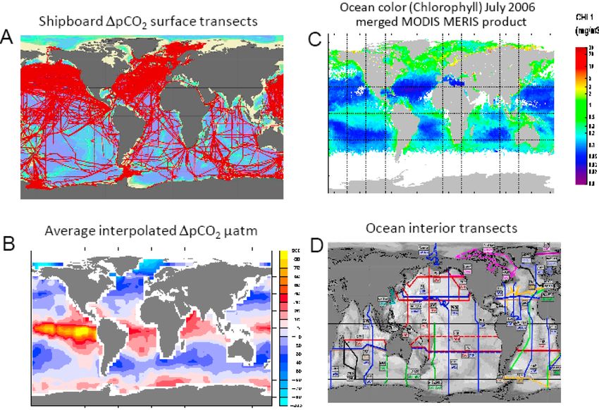
Figure 5. (A) Spatial sampling of surface ocean from research vessels and ships of opportunity observing 1pCO2 for air–sea flux (from
SOCAT). (B) Global 1pCO2 climatology synthesis obtained from these more than 6 million local measurements (Takahashi et al., 2009).
(C) Merged MERIS/MODIS ocean colour product (Chl a). (D) Transects of main ocean interior measurement campaigns (cross sections
from GO-SHIP plan).
3.4.2 Ocean interior measurements gram (GO-SHIP); www.go-ship.org). The current situation
is that data from these repeat occupations have already re-
vealed substantial changes in the ocean interior carbon stor-
In the late 1980s and early 1990s, carbon samples in the
age in response to the continuing uptake of anthropogenic
ocean interior were collected and analyzed from 95 research
CO2 (e.g., Wanninkhof et al., 2010; Sabine et al., 2008; Mu-
cruises run over about a 10 year period, part of the Joint
rata et al., 2007; Feely et al., 2012) as well as the presence of
Global Ocean Flux Study (JGOFS) and World Ocean Cir-
a substantial amount of decadal variability in the ocean car-
culation Experiment (WOCE) (Fig. 5). Based on these data,
bon cycle. In addition to documenting changes that already
Sabine et al. (2004) estimated that the total inventory of an-
occurred since the first occupation, these repeat hydrographic
thropogenic carbon that had accumulated in the ocean up
measurements continue to serve as a baseline to assess future
to 1994 was 118 ± 19 Pg C, accounting for 48 % of CO2 re-
changes. Repeat surveys of the ocean with physical parame-
leased from fossil fuel burning between 1800 and 1994. Re-
ter measurements are also suited to detect changes in oceanic
cent work shows that several marginal seas, not directly sam-
transport of heat, as well as changes in oxygen (Keeling et
pled by the data used by Sabine et al. (2004), stored more
al., 2010) and nutrients. Below the level of the ARGO array
anthropogenic carbon per unit area than the open ocean, and
of automated floats (www.argo.ucsd.edu/) repeat hydrogra-
that they contributed significant carbon to their adjacent ma-
phy is the only global method capable of observing long-term
jor ocean basins (Lee et al., 2011).
trends in ocean carbon. The program also provides data for
Systematic and global re-occupation of select hydro-
sensor calibration and to support continuing model develop-
graphic sections was initiated by the international commu-
ment that lead to improved forecasting skills for oceans and
nity in the early 2000s to quantify changes in storage and
global climate.
transport of heat, fresh water, carbon dioxide (CO2 ), and
For the global ocean, the Global Ocean Data Analysis
related parameters (internationally coordinated through the
Project (GLODAP) data set (Key et al., 2004) that assembled
Global Ocean Ship-Based Hydrographic Investigation Pro-
www.biogeosciences.net/11/3547/2014/ Biogeosciences, 11, 3547–3602, 20143560 P. Ciais et al.: Current systematic carbon-cycle observations
the data from the first global survey has become a benchmark carbon-related (1pCO2 , TA, pH, DIC) sensors for ocean use
for testing biogeochemical ocean general circulation models. on autonomous vehicles are being developed and tested.
It also has served as the basis for first data assimilation efforts
to estimate global-scale ocean–atmosphere CO2 fluxes (Gru- 3.4.4 Remote sensing of ocean carbon-cycle parameters
ber et al., 2009; Gloor et al., 2003). For different oceans or
ocean basins, new repeat hydrography data syntheses have For the oceans, remote sensing is critical for understanding
been created (e.g. CARbon dyoxide IN the Atlantic Ocean global patterns of ocean physics (e.g., temperature, dynamic
– CARINA, Key et al., 2010) or are emerging (e.g. PA- height), biology (e.g., ocean color), chemistry (e.g., salin-
CIFic ocean Interior CArbon – PACIFICA data set through ity) and air–sea forcing properties (e.g., surface winds, wave
the North Pacific Marine Science Organization (PICES) and height). Two long time series of satellite data have greatly
other partners). The data collected so far through the repeat contributed to a better estimation of carbon fluxes: the Ad-
hydrography program are too sparse to unambiguously doc- vanced Very High Resolution Radiometer (AVHRR) initi-
ument the global-scale accumulation of anthropogenic CO2 ated sea surface temperature (SST) since the early 1980s, and
since the 1990s, although the data collection PACIFICA is the Sea-viewing Wide Field-of-view Sensor (SeaWiFS) initi-
now finalized and published at http://cdiac.ornl.gov/oceans/ ated chlorophyll a concentration (a proxy of the phytoplank-
PACIFICA/ and ongoing synthesis work will likely resolve ton concentration in surface waters) available since the late
this challenge soon (e.g. Sabine and Tanhua, 2010). 1990s (http://oceancolor.gsfc.nasa.gov/) (McClain, 2009).
Currently, monitoring programs do not exist for oceanic These records advanced the understanding of the temporal
1pCH4 , as the ocean is considered to be only a minor source variability and spatial distribution of physical and biological
of this greenhouse gas (Ciais et al., 2013). However, the po- parameters in the ocean, leading to important improvements
tential for enhanced destabilization of CH4 gas hydrates un- in ocean modeling during the last decades. More recent sen-
der climate change requires attention, especially in vulnera- sors such as MODIS (Moderate-Resolution Imaging Spec-
ble regions such as coastal slopes and the Arctic (Biastoch et troradiometer) (Franz et al., 2006) and MERIS (MEdium-
al., 2011). Resolution Imaging Spectrometer) (Rast et al., 1999) have
strengthened and extended this space-based ocean observing
system (Fig. 5). A third satellite data product of high impor-
3.4.3 Ocean in situ biological measurements related to
tance for ocean carbon-cycle studies are direct wind speed
carbon cycle
measurements from a range of scatterometers, such as Quick
Scatterometer – QuikSCAT/SeaWinds (http://winds.jpl.nasa.
Primary production, carbon and nitrogen fixation, gov/missions/quikscat/).
metabolism, and biological species composition con- Currently, estimating air–sea CO2 fluxes from combined
tribute to an understanding of the ocean carbon cycle. Those satellite and in situ measurements remains a challenge be-
biological observations provide insight to marine population- cause the carbon content in the ocean surface layer de-
and community-level changes and could ultimately lead pends not only on the surface temperature and phytoplankton
to development of biological indicators, for example to biomass (that can be monitored from space), but also on the
characterize the biological effects of ocean acidification. In mixed layer depth and water-mass history. Recent attempts
addition, measurements of ocean partial pressure of N2 O that combine satellite data and model simulation showed the
and CH4 on research cruises have enabled partial/regional potential of this approach (Telszewski et al., 2009). Develop-
estimates of air–sea fluxes of these greenhouse gases. New ment of operational ocean circulation models associated with
observations of O2 vertical profiles within the ocean from satellite products will probably lead to an acceleration of
ARGO free-drifting buoys have shown promising results, the use of these approaches to routinely produce ocean CO2
and an increase in the number of buoys carrying O2 sensors fluxes. In the near term, these methods will benefit from the
is expected as the technology improves the reliability and sea surface salinity (SSS) measurement using the Soil Mois-
power consumption (Gruber et al., 2010). The development ture Ocean Salinity (SMOS) sensor launched in 2009, and
of optical sensors has allowed the measurement of phy- the Aquarius sensor launched in 2011. In regions affected by
toplankton fluorescence onboard ARGO buoys (Johnson the discharge of large rivers, such as the equatorial Atlantic
et al., 2009; Claustre et al., 2010) providing a new tool with the Amazon and Congo rivers’ plumes, the thermody-
to monitor biological productivity, and thus the carbon namic processes that control 1pCO2 depend not only on the
cycle, within the ocean interior. The increase in the number SST but also on the SSS (De La Paz et al., 2010).
of bio-optical ARGO buoys in forthcoming years will New satellite products are expected to enhance ocean
complement available satellite ocean color data of surface color products. The detection of the phytoplankton functional
chlorophyll concentration. Furthermore, the advent of pH types is an example of product useful to better understand
and nitrate sensors provides the potential to expand the the biological pump of carbon in the ocean (Alvain et al.,
suite of measurements to assess the trophic status as well 2005; Uitz et al., 2010), because phytoplankton species play
as ocean acidification (Johnson et al., 2009). A number of very different role in carbon uptake and export. All these
Biogeosciences, 11, 3547–3602, 2014 www.biogeosciences.net/11/3547/2014/You can also read