Deep Gaussian Scale Mixture Prior for Spectral Compressive Imaging
←
→
Page content transcription
If your browser does not render page correctly, please read the page content below
Deep Gaussian Scale Mixture Prior for Spectral Compressive Imaging

                                                        Tao Huang1 Weisheng Dong1 * Xin Yuan2 * Jinjian Wu1 Guangming Shi1
                                                               1
                                                                 School of Artificial Intelligence, Xidian University 2 Bell Labs
                                                     thuang 666@stu.xidian.edu.cn                wsdong@mail.xidian.edu.cn           xyuan@bell-labs.com
                                                                           jinjian.wu@mail.xidian.edu.cn          gmshi@xidian.edu.cn
arXiv:2103.07152v2 [eess.IV] 30 Mar 2021

                                                                         Abstract

                                              In coded aperture snapshot spectral imaging (CASSI)
                                           system, the real-world hyperspectral image (HSI) can be re-
                                           constructed from the captured compressive image in a snap-
                                           shot. Model-based HSI reconstruction methods employed
                                           hand-crafted priors to solve the reconstruction problem, but
                                           most of which achieved limited success due to the poor rep-
                                           resentation capability of these hand-crafted priors. Deep
                                           learning based methods learning the mappings between the
                                           compressive images and the HSIs directly achieved much
                                           better results. Yet, it is nontrivial to design a powerful deep
                                           network heuristically for achieving satisfied results. In this
                                           paper, we propose a novel HSI reconstruction method based
                                           on the Maximum a Posterior (MAP) estimation framework
                                           using learned Gaussian Scale Mixture (GSM) prior. Dif-            Figure 1. A single shot measurement captured by [22] and 28 re-
                                                                                                             constructed spectral channels using our proposed method.
                                           ferent from existing GSM models using hand-crafted scale
                                           priors (e.g., the Jeffrey’s prior), we propose to learn the
                                           scale prior through a deep convolutional neural network
                                                                                                             tional imaging systems with single 1D or 2D sensor require
                                           (DCNN). Furthermore, we also propose to estimate the lo-
                                                                                                             a long time to scan the scene, failing to capture dynamic
                                           cal means of the GSM models by the DCNN. All the pa-
                                                                                                             objects. Recently, many coded aperture snapshot spectral
                                           rameters of the MAP estimation algorithm and the DCNN
                                                                                                             imaging (CASSI) systems [8, 22, 23, 35] have been pro-
                                           parameters are jointly optimized through end-to-end train-
                                                                                                             posed to capture the 3D HSIs at video rate. CASSI utilizes
                                           ing. Extensive experimental results on both synthetic and
                                                                                                             a physical mask and a disperser to modulate different wave-
                                           real datasets demonstrate that the proposed method outper-
                                                                                                             length signals, and mixes all modulated signals to generate
                                           forms existing state-of-the-art methods. The code is avail-
                                                                                                             a single 2D compressive image. Then a reconstruction al-
                                           able at https://see.xidian.edu.cn/faculty/
                                                                                                             gorithm is employed to reconstruct the 3D HSI from the
                                           wsdong/Projects/DGSM-SCI.htm.
                                                                                                             2D compressive image. As shown in Fig. 1, 28 spectral
                                                                                                             bands have been reconstructed from a 2D compressive im-
                                                                                                             age (measurement) captured by a real CASSI system [22].
                                           1. Introduction                                                      Therefore, reconstruction algorithms play a pivot role in
                                               Compared with traditional RGB images, hyperspectral           CASSI. To solve this ill-posed inverse problem, previous
                                           images (HSIs) have more spectral bands and can describe           model-based methods adopted hand-crafted priors to reg-
                                           the characteristics of material in the imaged scene more ac-      ularize the reconstruction process. In GAP-TV [43], the
                                           curately. Relying on its rich spectral information, HSIs are      total variation prior was introduced to solve the HSI recon-
                                           beneficial to many computer vision tasks, e.g., object recog-     struction problem. Based on the assumption that HSIs have
                                           nition [33], detection [40] and tracking [34]. The conven-        sparse representations with respective to some dictionaries,
                                                                                                             sparse-based methods [14, 17, 35] exploited the `1 sparsity
                                              * Corresponding authors.                                       to regularize the solution. Considering that the pixels of
HSIs have strong long-range dependence, non-local based           2.1. Conventional model-based HSI reconstruction
methods [18, 38, 48] have also been proposed. However,                  methods
the model-based methods have to tweak parameters manu-
                                                                     Reconstructing the 3D HSI from the 2D compressive im-
ally, resulting in limited reconstruction quality in addition
                                                                  age is the core of CASSI system and usually with the help
to the slow reconstruction speed. Inspired by the successes
                                                                  of various hand-crafted priors. In [7] gradient projection
of deep convolutional neural networks (DCNNs) for natu-
                                                                  algorithms were proposed to solve the sparse HSI recon-
ral image restoration [16, 47], deep learning based HSI re-
                                                                  struction problems. In [17] dictionary learning based sparse
construction methods [3, 36, 37] have also been proposed.
                                                                  regularizers have been employed for HSI reconstruction. In
In [36], an iterative HSI reconstruction algorithm was un-
                                                                  [1, 14, 43] total variation (TV) regularizers have also been
folded into a DCNN, where two sub-networks were used to
                                                                  adopted to suppress the noise and artifacts. In [18], the
exploit the spatial-spectral priors. In [37] the nonlocal self-
                                                                  nonlocal self-similarity and the low-rank property of HSIs
similarity prior has also been incorporated to further im-
                                                                  have been exploited, leading to superior HSI reconstruction
prove the results. In addition to the optimization-inspired
                                                                  performance. The major drawbacks of these model-based
methods, DCNN-based methods [22, 24, 41] that learned
                                                                  methods are that they are time-consuming and need to se-
the mapping functions between the 2D measurements and
                                                                  lect the parameters manually.
the 3D HSIs directly have also been proposed. λ-net [24]
reconstructed the HSIs from the inputs of 2D measurements         2.2. Deep learning-based HSI reconstruction
and the mask through a two-stage DCNN. TSA-Net [22] in-
                                                                      Due to the powerful learning ability, deep neural net-
tegrated three spatial-spectral self-attention modules in the
                                                                  works treating the HSI reconstruction as a nonlinear map-
backbone U-Net [31] and achieved state-of-the-art results.
                                                                  ping problem have achieved much better results than model-
Although promising HSI reconstruction performance has
                                                                  based methods. In [41] initial estimates of the HSIs were
been achieved, it is non-trivial to design a powerful DCNN
                                                                  first obtained by the method of [1] and were further refined
heuristically.
                                                                  by a DCNN. λ-net [24] reconstructed the HSIs through a
    Bearing the above concerns in mind, in this paper, we
                                                                  two-stage procedure, where the HSIs were first initially re-
propose an interpretable HSI reconstruction method with
                                                                  constructed by a Generative Adversarial Network (GAN)
learned Gaussian Scale Mixture (GSM) prior. The contri-
                                                                  with self-attention, followed by a refinement stage for fur-
butions of this paper are listed as follows.
                                                                  ther improvements. In [22], DCNN with spatial-spectral
   • Learned GSM models are proposed to exploit the               self-attention modules was proposed to exploit the spatial-
     spatial-spectral correlations of HSIs. Unlike the exist-     spectral correlation, leading to state-of-the-art performance.
     ing GSM models with hand-crafted scale priors (e.g.,         Instead of designing the DCNN heuristically, DCNNs based
     Jeffrey’s prior), we propose to learn the scale prior by     on unfolding optimization-based HSI reconstruction algo-
     a DCNN.                                                      rithms have also been proposed [21]. In [36] a HSI recon-
                                                                  struction algorithm with a denoising prior was unfolded into
   • The local means of the GSM models are estimated as
                                                                  a deep neural network. Since the spatial-spectral prior has
     a weighted average of the spatial-spectral neighboring
                                                                  not been fully exploited, the method of [36] achieved lim-
     pixels. The spatial-spectral similarity weights are also
                                                                  ited success. To exploit the nonlocal self-similarity of HSIs,
     estimated by the DCNN.
                                                                  the nonlocal sub-network has also been integrated into the
   • The HSI reconstruction problem is formulated as a            deep network proposed in [37], leading to further improve-
     Maximum a Posteriori (MAP) estimation problem                ments. The other line of work is to apply deep denoiser
     with the learned GSM models. All the parameters in           into the optimization algorithm, leading to a plug-and-play
     the MAP estimator are jointly optimized in an end-to-        framework [49].
     end manner.
                                                                  2.3. GSM models for signal modeling
   • Extensive experimental results on both synthetic and
                                                                     As a classical probability model, the Gaussian Scale
     real datasets show that the proposed method out-
                                                                  Mixture (GSM) model has been used for various image
     performs existing state-of-the-art HSI reconstruction
                                                                  restoration tasks. In [27] the GSM model was utilized to
     methods.
                                                                  characterize the distributions of the wavelet coefficients for
2. Related Work                                                   image denoising. In [5] the GSM model has been proposed
                                                                  to model the sparse codes for simultaneous sparse coding
   Hereby, we briefly review the conventional model-based         with applications to image restoration. In [26, 32] the GSM
HSI reconstruction methods, the recently proposed deep            models have also been used to model the moving objects
learning-based HSI reconstruction methods and the GSM             of videos for foreground estimation, achieving state-of-the-
models for signal modeling.                                       art performance. In this paper, we propose to character-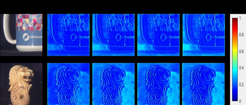
ize distributions of the HSIs with the GSM models for HSI       L − 1), and A ∈ RM ×N denotes the measurement matrix of
reconstruction. Different from existing GSM models with         the CASSI system, implemented by the coded aperture and
manually selected scale priors, we propose to learn both the    disperser. Considering the measurement noise n ∈ RM , the
scale prior and local means of the GSM models with DC-          forward model of CASSI is now
NNs. Through end-to-end training, all the parameters are
learned jointly.                                                                         y = Ax + n.                        (5)

                                                                The theoretical performance bounds of CASSI have been
                                                                derived in [12].

                                                                4. The Proposed Method
                                                                4.1. GSM models for CASSI
                                                                   We formulate the HSI reconstruction as a maximum a
                                                                posteriori (MAP) estimation problem. Given the observed
      Figure 2. The imaging schematic of CASSI system.          measurement y, the desired 3D HSI x can be estimated by
                                                                maximizing the posterior
3. The CASSI Observation Model
                                                                            log p(x|y) ∝ log p(y|x) + log p(x),             (6)
    As shown in Fig. 2, the 3D HSI is encoded into the 2D
compressive image by the CASSI system. In the CASSI             where p(y|x) is the likelihood term and p(x) is the (to be
system, the 3D spectral data cube is first modulated spa-       determined) prior distribution of x. The likelihood term is
tially by a coded aperture (i.e., a physical mask). Then,       generally modeled with a Gaussian function as
the following dispersive prism disperses each wavelength                                 1

                                                                                                    ||y−Ax||2

of the modulated data. A 2D imaging sensor captures the                    p(y|x) = √2πσ     exp − 2σ2 2 .              (7)
dispersed data and outputs a 2D measurement which mixes
the information of all wavelengths.                             For the prior term p(x), we propose to characterize each
    Let X ∈ RH×W ×L denote the 3D spectral data cube and        pixel xi of the HSI with a nonzero-mean Gaussian distri-
C ∈ RH×W denote the physical mask. The lth wavelength           bution of standard deviation θi . With a scale prior p(θi )
of the modulated image can thus be represented as               and the assumption that θi and xi are independent, we can
                                                                model x with the following GSM model
                         0
                       Xl = C       Xl ,                 (1)               Q                    R∞
                                                                   p(x) = i p(xi ), p(xi ) = 0 p(xi |θi )p(θi )dθi , (8)
        0
where X ∈ RH×W ×L is the 3D modulated image and
                                                                where p(xi |θi ) is a nonzero-mean Gaussian distribution
denotes the element-wise product. In CASSI system, the
                                                                with variance θi2 and mean ui , i.e.,
modulated image is dispersed by the dispersive prism. In
                                          0
other words, each channel of the00tensor X will be shifted                   p(xi |θi ) =   √1
                                                                                                             −ui )
                                                                                                    exp(− (xi2θ
                                                                                                                   2
                                                                                                                   ).       (9)
                                                                                                                2
spatially and the shifted tensor X ∈ RH×(W +L−1)×L can                                       2πθi              i

be written as                                                   With different scale priors, the GSM model can well express
                 00             0                               many distributions.
               X (r, c, l) = X (r, c + dl , l),          (2)
                                                                    Regarding the scale prior p(θi ), instead of modeling
where dl denotes the shifed distance of the lth channel, 1 ≤    p(θi ) with an exact prior (e.g., the Jeffrey’s prior p(θi ) =
                                                                 1
r ≤ H, 1 ≤ c ≤ W and 1 ≤ l ≤ L. At last, the 2D imaging         θi ), we introduce a general form as
sensor captures the shifted image into a 2D measurement
                                                                                     p(θi ) ∝ exp(−J(θi )),                (10)
(by compressing the spectral domain), as
                           PL      00                           where the J(θi ) is an energy function. Instead of computing
                      Y = l=1 Xl ,                        (3)
                                                                an analytical expression of p(xi ) that is often intractable, we
where Y ∈ RH×(W +L−1) represents the 2D measurement.            propose to jointly estimate x and θ by replacing p(x) with
As such, the matrix-vector form of Eq. (3) can be formu-        p(x, θ) in the MAP estimator. This is
lated as
                                                                  (x, θ) = argmaxx,θ log p(y|x) + log p(x, θ)
                        y = Ax,                       (4)
                                                                         = argmax log p(y|x) + log p(x|θ) + log p(θ).
where x ∈ RN and y ∈ RM denote the vectorized form                             x,θ
of X and Y respectively, N = HW L and M = H(W +                                                                            (11)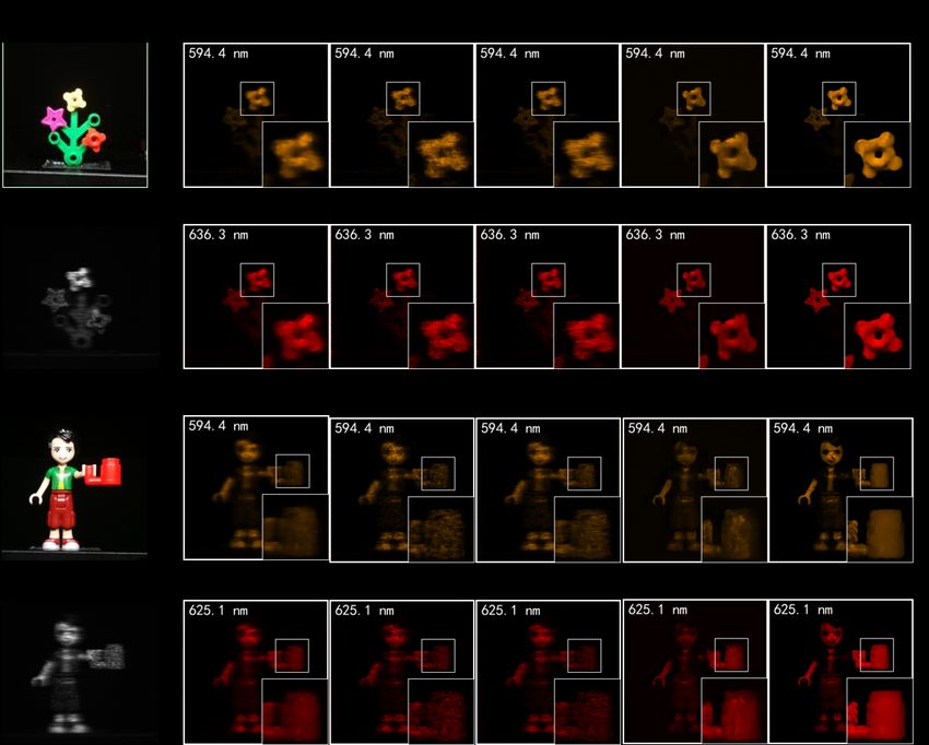
By substituting the Gaussian likelihood term of Eq. (7) and             4.2. Deep GSM for CASSI
the prior terms of p(xi |θi ) and p(θi ) into the above MAP
                                                                           In general, alternating computing x and w requires nu-
estimator, we can obtain the following objective function
                                                                        merous iterations to converge and it is necessary to impose
                                               N                        a hand-crafted prior of p(θ). Moreover, all the algorithm
                                              X   1                     parameters and the 3D filters cannot be jointly optimized.
   (x, θ) = argmin ||y − Ax||22 + σ 2               2 (xi − ui )
                                                                2
               x,θ                            i=1
                                                  θi                    To address these issues, we propose to optimize x and w
                               PN                                       jointly by a DCNN. For network design purpose, we re-
                      + 2σ 2     i=1   log θi + 2σ 2 J(θ)
                                                                        bridge the x and w-subproblems via a united framework
                                               N
                                              X   1
          = argmin ||y − Ax||22 + σ 2              2 (xi − ui )
                                                               2
                                                                        x(t+1) = x(t) − 2δ{A> (Ax(t) − y) + S(x(t) )(x(t) − u(t) )},
               x,θ                               θ
                                              i=1 i                                                                             (17)
                      + R(θ),                                    (12)   where S(·) represents the function of the DCNN for esti-
                                                                        mating w, i.e., the solution of (16). As shown in Fig. 3(a),
                    PN
where R(θ) = 2σ 2 i=1 log θi + 2σ 2 J(θ). Thereby, the                  we construct the end-to-end network with T stages corre-
HSI reconstruction problem can be solved by alternating                 sponding to T iterations for iteratively optimizing x and w.
optimizing x and θ.                                                     The proposed network consists of the following main mod-
   For the x-subproblem, with fixed θ, we can solve x by                ules.
solving                                                                   • The measurement y is split into a 3D data cube of size
                                    PN                                      H × W × L to initialize x.
  x = argminx ||y − Ax||22 +            i=1   wi (xi − ui )2 ,   (13)
                                                                          • We use two sub-networks to learn the measurement
              2
where wi = σθ2 and the mean ui keeps updating with x. In-                   matrix A and its transposed version A> .
               i
spired by the auto-regressive (AR) model [6], we can calcu-
                                                                          • For estimating w, we develop a lightweight variant
late the weighted average of the local spatial-spectral neigh-
                                                                            of U-Net and a weight generator to learn the function
boring pixels as the estimation of the mean ui , i.e.,
                                                                            S(·).
                         ui = ki> xi ,                           (14)     • Instead of using a manually designed method to learn
                  3
                                                                            the 3D filters, we utilize the same lightweight U-Net
where ki ∈ Rq denotes the vectorized 3D filter of size                      and a 3D filter generator to generate the spatially-
                               3
q × q × q for xi and xi ∈ Rq represents the local spatial-                  variant filters. According to Eq. (14), we filter the
spectral neighboring pixels of xi . For the 3D filters, some                current x by the generated 3D filters for updating the
existing methods (e.g., the guided filtering [9, 15], the non-              means u.
local means methods [2, 4] or the deep learning based
method [25]) can be used to estimate the spatially-variant              4.3. Network Architecture
filters.                                                                    Considering that the real system has large spatial size
    To solve Eq. (13), we employ gradient descent as                    of the mask and measurements (e.g., the mask and mea-
                                                                        surements of [22] are 660 × 660 and 660 × 714), the net-
x(t+1) = x(t) − 2δ{A> (Ax(t) − y) + w(t) (x(t) − u(t) )},               work training with explicitly constructed A and A> requires
                                                    (15)                a large amount GPU memory and computational complex-
where u(t) = [ut1 , · · · , utN ]> ∈ RN , w(t) =                        ity. To address this issue, we propose to learn these two
                t >
[w1t , · · · , wN ] ∈ RN and δ is the step size.                        operations with two sub-networks.
    The θ-subproblem can be changed to estimate w. With
fixed x, w can be estimated by                                          The modules for learning the measurement matrix A
                      PN                                                and A> . Learning A and A> with sub-networks allows
     w = argminw         i=1   wi (xi − ui )2 + R(w).            (16)   one to train them on small patches (e.g., 64 × 64 or 96 × 96)
                                                                        that can greatly reduce memory consumption and computa-
The solution of w depends on R(w) being used. For some                  tional complexity. Furthermore, we can train a sub-network
priors, a closed-form solution can be achieved [26]; for oth-           to learn multiple masks such that the trained network can
ers, iterative algorithms might be used. However, each of               work well on multiple imaging systems. The measurement
them has their pros and cons. To cope with this challenge,              matrix A represents a hybrid operator of modulation, i.e.,
hereby instead of using a manually designed proximal op-                shifting and summation, which can be implemented by two
erator, we propose to estimate w(t+1) from x(t+1) using a               Conv layers and four ResBlocks followed by shifting and
DCNN as will be described in the next subsection.                       summation operations. As shown in Fig. 3(b), x is fed into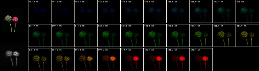
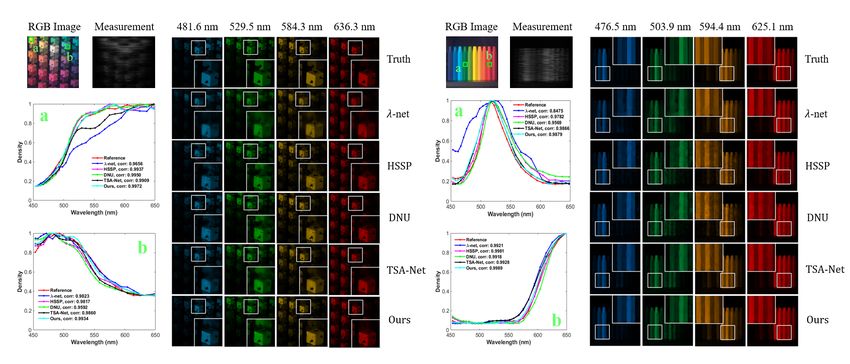
Figure 3. Architecture of the proposed network for hyperspectral image reconstruction. The architectures of (a) the overall network, (b)
the measurement matrix, (c) the transposed version of the measurement matrix, (d) the weight generator, and (e) the filter generator.

the sub-network to generate modulated feature maps that                Fig. 3 (d). Some weight maps w of two HSIs estimated in
are further shifted and summed along the spectral dimen-               the fourth stage are visualized (with normalization) in Fig.
sion to generate the measurements y = Ax. Each ResBlock                4. From Fig. 4, we can see that w vary spatially and are
[11] consists of 2 Conv layers with a ReLU nonlinearity                consistent with the image edges and textures. Aided by this
function plus a skip connection. Regarding A> , as shown               well-learned w, the proposed method will pay attentions to
in Fig. 3(c), we first slide a H × W extraction window on              the edges and textures.
the input y of size H × (W + L − 1) with the slide step
one pixel and split the input into L-channel image of size
H × W . Then the split sub-images are fed into two Conv
layers and four ResBlocks to generate the estimate A> y.

The module for estimating the regularization param-
eters w. As shown in the Fig. 3 (a), we propose a
lightweight U-Net consisting of five encoding blocks (EBs)
and four decoding blocks (DBs) to estimate the weights
w(t) from the current estimate x(t) . Each EB and DB con-              Figure 4. The visualization of the regularization parameters w es-
tains two Conv layers with ReLU nonlinearity function. The             timated in the 4-th stage. Left: the corresponding RGB image;
average pooling layer with a stride of 2 is inserted between           right: the w images associated with the four spectral bands.
every two neighboring EBs to downsample the feature maps
and a bilinear interpolation layer with a scaling factor 2 is
adopted ahead of every DB to increase the spatial resolu-              The module for estimating the local means u. We es-
tions of the feature maps. We have noticed that the average            timate the means of GSM models following Eq. (14). To
pooling works better than max pooling in our problem and               estimate the spatial-variant 3D filters, we add a filter gen-
the bilinear interpolation plays an important role in DBs.             erator with the input of the feature maps generated by the
3 × 3 Conv filters are used in all the Conv layers. The                U-net, as shown in Fig. 3(a). Estimating the spatially adap-
channel numbers of the output features of the 5 EBs and                tive 3D filters has advantages in adapting to local HSI edges
4 DBs are set to 32, 64, 64, 128, 128, 128, 64, 64 and 32,             and texture structures. However, directly generating these
respectively. To alleviate the gradient vanishing problem,             3D filters will cost a large amount of GPU memory that is
the feature maps of the first EB are connected to first EB             unaffordable. To reduce the GPU memory consumption,
of the U-net of the subsequent stages. The feature maps of             we propose to factorize each 3D filter into three 1D filters,
the last DB are fed into a weight generator that contains 2            expressed as
3 × 3 Conv layers to generate the weights w as shown in                                      Ki = ri ⊗ ci ⊗ si ,                    (18)

where Ki ∈ Rq×q×q denotes the 3D filter, ri ∈ Rq , ci ∈ Rq            During training, to simulate the measurements, we first
and si ∈ Rq denote the three 1D filters corresponding to          randomly extract 96 × 96 × 28 patches from the training
the three dimensions, respectively, and ⊗ denotes the ten-        dataset as training labels (ground truth HSI) and randomly
sor product. In this way, filtering the local neighbors Xi        extract 96 × 96 patches from the real mask to generate the
with the 3D filter Ki can be transformed into convoluting         modulated data. Then the modulated data is shifted in spa-
the local neighbors with the three 1D filters along three di-     tial at an interval of two pixels. The spectral dimension of
mensions in sequence. By factorizing each 3D filter into          the shifted data is summed up to generate the 2D measure-
three 1D filters we can reduce the number of filter coeffi-       ments of size 96 × 150 as the network inputs. We use Ran-
cients from N · q 3 to 3 · N · q, and thus significantly reduce   dom flipping and rotation for data argumentation. The peak-
the GPU memory cost and the computational complexity.             signal-to-noise (PSNR) and the structural similarity index
As shown in Fig. 3(e), the filter generator contains three        (SSIM) [39] are both employed to evaluate the performance
branches to learn the 1D filters, respectively. After generat-    of the HSI reconstruction methods.
ing the filters, we can compute the means of GSM models
following Eq. (14).                                               5.2. Comparison with State-of-the-Art Methods

4.4. Network training                                                We compare the proposed HSI reconstruction method
                                                                  with several state-of-the-art methods, including three
   We jointly learn the network parameters Θ through end-         model-based methods (i.e., TwIST [1], GAP-TV [43] and
to-end training. Except the step size δ, all the network pa-      DeSCI [18]) and four deep learning based methods (i.e., λ-
rameters of each stage are shared. All the parameters are         net [24], HSSP [36], DNU [37] and TSA-Net [22]). As the
optimized by minimizing the following loss function               source codes are unavailable, we re-implemented HSSP and
                      1
                        PD                                        DNU by ourselves. For other competing methods, we use
     Θ̂ = argminΘ D       d=1 kF(yd ; Θ) − xd k1 ,      (19)
                                                                  the source codes released by their authors. For the sake of
where D denotes the total number of the training samples,         fair comparison, all deep learning methods were re-trained
F(yd ; Θ) represents the output of the proposed network           on the same training dataset. Table 1 shows the reconstruc-
given dth measurement yd and the network parameters Θ,            tion results of these testing methods on the 10 scenes, where
and xd is the ground-truth HSI. The ADAM optimizer [13]           we can see that the deep learning-based methods outper-
with setting β1 = 0.9, β2 = 0.999 and  = 10−8 is ex-             form the model-based methods. The proposed method out-
ploited to train the proposed network. We set the learning        performs other deep learning-based methods by a large mar-
rate as 10−4 . The parameters of the convolutional layers are     gin. Specifically, our method outperforms the second best
initialized by the Xavier initialization [10]. We implement       method TSA-Net by 1.17dB in average PSNR and 0.0227
the proposed method in PyTorch and train the network using        in average SSIM. Compared with the two deep unfolding
a single Nvidia Titan XP GPU. Instead of using the `2 norm        methods HSSP and DNU, the improvements by the pro-
in the loss function, here we use the `1 norm that has been       posed method over HSSP [36] and DNU [37] are 2.28 dB
proved to be better in preserving image edges and textures.       and 1.89 dB in average, respectively. The HSSP and DNU
                                                                  methods also tried to learn the spatial-spectral correlations
5. Simulation Results                                             of HSIs by two sub-networks without emphasizing image
                                                                  edges and textures. By contrast, we propose to learn the
5.1. Experimental Setup                                           spatial-spectral prior of HSIs by the spatially-adaptive GSM
   To verify the effectiveness of the proposed HSI recon-         models characterized by the learned local means and vari-
struction method for CASSI, we conduct simulations on             ances. The learned GSM models have advantages in adapt-
two public HSI datasets CAVE [42] and KAIST [3]. The              ing to various HSI edges and textures. Fig. 5 plots se-
CAVE dataset consists of 32 HSIs of spatial size 512 × 512        lected frames and spectral curves of the reconstructed HSIs
with 31 spectral bands. The KAIST dataset has 30 HSIs             by the five deep learning-based methods. We can see that
of spatial size 2704 × 3376 also with 31 spectral bands.          the HSIs reconstructed by the proposed method have more
Similar to TSA-Net [22], we employ the real mask of size          edge details and less undesirable visual artifacts than the
256 × 256 for simulation. Following the procedure in TSA-         other methods. The RGB images of the 10 scenes and more
Net [22], the CAVE dataset is used for network training, and      visual comparison results are shown in the supplementary
10 scenes of spatial size 256 × 256 from the KAIST dataset        material (SM).
are extracted for testing. To be consistent with the wave-
                                                                  5.3. Multiple Mask Results
length of the real system [22], we unify the wavelength of
the training and testing data by spectral interpolation. Thus,       As mentioned before, our proposed network is robust to
the modified training and testing data have 28 spectral bands     mask due to the learning of A and A> . To verify this, we
ranging from 450nm to 650nm.                                      conducted experiments on compound training and testing
Table 1. The PSNR in dB (left entry in each cell) and SSIM (right entry in each cell) results of the test methods on 10 scenes.
Method TwIST [1] GAP-TV [43] DeSCI [18] λ-net [24] HSSP [36] DNU [37] TSA-Net [22] Ours
Scene1 25.16, 0.6996 26.82, 0.7544 27.13, 0.7479 30.10, 0.8492 31.48, 0.8577 31.72, 0.8634 32.03, 0.8920 33.26, 0.9152
Scene2 23.02, 0.6038 22.89, 0.6103 23.04, 0.6198 28.49, 0.8054 31.09, 0.8422 31.13, 0.8464 31.00, 0.8583 32.09, 0.8977
Scene3 21.40, 0.7105 26.31, 0.8024 26.62, 0.8182 27.73, 0.8696 28.96, 0.8231 29.99, 0.8447 32.25, 0.9145 33.06, 0.9251
Scene4 30.19, 0.8508 30.65, 0.8522 34.96, 0.8966 37.01, 0.9338 34.56, 0.9018 35.34, 0.9084 39.19, 0.9528 40.54, 0.9636
Scene5 21.41, 0.6351 23.64, 0.7033 23.94, 0.7057 26.19, 0.8166 28.53, 0.8084 29.03, 0.8326 29.39, 0.8835 28.86, 0.8820
Scene6 20.95, 0.6435 21.85, 0.6625 22.38, 0.6834 28.64, 0.8527 30.83, 0.8766 30.87, 0.8868 31.44, 0.9076 33.08, 0.9372
Scene7 22.20, 0.6427 23.76, 0.6881 24.45, 0.7433 26.47, 0.8062 28.71, 0.8236 28.99, 0.8386 30.32, 0.8782 30.74, 0.8860
Scene8 21.82, 0.6495 21.98, 0.6547 22.03, 0.6725 26.09, 0.8307 30.09, 0.8811 30.13, 0.8845 29.35, 0.8884 31.55, 0.9234
Scene9 22.42, 0.6902 22.63, 0.6815 24.56, 0.7320 27.50, 0.8258 30.43, 0.8676 31.03, 0.8760 30.01, 0.8901 31.66, 0.9110
Scene10 22.67, 0.5687 23.10, 0.5839 23.59, 0.5874 27.13, 0.8163 28.78, 0.8416 29.14, 0.8494 29.59, 0.8740 31.44, 0.9247
Average 23.12, 0.6694 24.36, 0.6993 25.27, 0.7207 28.53, 0.8406 30.35, 0.8524 30.74, 0.8631 31.46, 0.8939 32.63, 0.9166
Figure 5. Reconstructed images of Scene 2 (left) and Scene 9 (right) with 4 out of 28 spectral channels by the five deep learning-based
methods. Two regions in each scene are selected for analysing the spectra of the reconstructed results. Zoom in for better view.
Table 2. The average PSNR (left) and SSIM (right) results with that were trained specifically for each mask, verifying the
five masks by the competing methods.
advantages of learning the measurement matrix A and A> .
Method DNU [37] TSA-Net [22] Ours
mask1 30.29, 0.8588 30.96, 0.8804 31.38, 0.8979
mask2 30.46, 0.8516 31.23, 0.8875 31.73, 0.9034
5.4. Ablation Study
mask3 30.80, 0.8663 31.43, 0.8904 31.81, 0.9055 We conduct several ablation studies to verify the impacts
mask4 30.65, 0.8610 31.15, 0.8863 31.58, 0.9038 of different modules of the proposed network, including the
mask5 30.74, 0.8631 31.46, 0.8939 31.70, 0.9018
choices of the filter sizes, number of stages and the use of
dense connections.
datasets that were simulated by applying 5 different masks. Fig. 7 (a) shows the results with different filter sizes,
The 5 masks of size 256×256 were extracted at the four cor- where we can see that larger filter size can improve the HSI
ners and the center of the real captured mask [22]. We only reconstruction quality. The improvement flattens out after
trained a single model by the proposed network on the com- q = 7 and thus we set q = 7 in our implementation. The
pound training dataset to deal with multiple masks, whereas results with different number of stages are shown in Fig. 7
we trained five different models associated with each mask (b), from which we observe that increasing the stage num-
by the DNU [37] and TSA-Net [22] methods on the datasets ber T leads to better performance. We set T = 4 in our im-
generated by the corresponding mask, respectively. Table 2 plementation for achieving a good trade-off between recon-
shows the average PSNR and SSIM results by these test- struction performance and computational complexity. We
ing methods on the 10 scenes. We can see that the pro- have also conducted a comparison between the proposed
posed method (only trained once on the compound training network without and with dense connections. The compar-
dataset) still outperforms the other two competing methods ison demonstrates that using dense connections can boostFigure 6. Reconstructed images of the real scene (Scene 4) with 28 spectral channels by the proposed method. Zoom in for better view.
Figure 7. Ablation study on the effects of (a) the filter size; (b) the
number of stage.
PSNR from 30.52dB to 32.63dB and SSIM from 0.8802 to
0.9166.
6. Real Data Results
We now apply the proposed method on the real SD-
CASSI system [22] which captures the real scenes with 28
wavelengths ranging from 450nm to 650nm and has 54- Figure 8. Reconstructed images of two real scenes (Scene 1 and
pixel dispersion in the column dimension. Thus, the mea- Scene 3) with 2 out of 28 spectral channels by the competing meth-
surements captured by the real system have a spatial size of ods. Zoom in for better view.
660 × 714. Similar to TSA-Net [22], we re-trained the pro-
posed method on all scenes of CAVE dataset and KAIST scale prior of GSM by a DCNN. Furthermore, motivated by
dataset. To simulate the real measurements, we injected 11- the auto-regressive model, the means of the GSM models
bit shot noise during training. We compare the proposed have been estimated as a weighted average of the spatial-
method with TwIST [1], GAP-TV [43], DeSCI [18] and spectral neighboring pixels, and these filter coefficients are
TSA-Net [22]. Visual comparison results of the compet- estimated by a DCNN as well aiming to learn sufficient
ing methods are shown in Fig. 8. It can be observed that the spatial-spectral correlations of HSIs. Extensive experimen-
proposed method can recover more details of the textures tal results on both synthetic and real datasets demonstrate
and suppress more noise. Fig. 1 and 6 show reconstructed that the proposed method outperforms existing state-of-the-
images of two real scenes (Scene 3 and Scene 4) with 28 art algorithms.
spectral channels by the proposed method. More visual re- Our proposed network is not limited to the spectral com-
sults are shown in the SM. pressive imaging such as CASSI and similar systems [46,
20], it can also be used in the video snapshot compres-
7. Conclusions sive imaging systems [28, 30, 29, 45]. Our work is paving
the way of real applications of snapshot compressive imag-
We have proposed an interpretable hyperspectral image
ing [19, 44].
reconstruction method for coded aperture snapshot spectral
imaging. Different from existing works, our network is in-
spired by the Gaussian scale mixture prior. Specifically, Acknowledgments. This work was supported in part by
the desired hyperspectral images were characterized by the the National Key R&D Program of China under Grant
GSM models and then the reconstruction problem was for- 2018AAA0101400 and the Natural Science Foundation
mulated as a MAP estimation problem. Instead of using of China under Grant 61991451, Grant 61632019, Grant
a manually designed prior, we have proposed to learn the 61621005, and Grant 61836008.References snapshot spectral imagers. Applied optics, 49(36):6824–
6833, 2010. 1, 2
[1] José M Bioucas-Dias and Mário AT Figueiredo. A new twist: [15] Shutao Li, Xudong Kang, and Jianwen Hu. Image fusion
Two-step iterative shrinkage/thresholding algorithms for im- with guided filtering. IEEE Transactions on Image process-
age restoration. IEEE Transactions on Image processing, ing, 22(7):2864–2875, 2013. 4
16(12):2992–3004, 2007. 2, 6, 7, 8 [16] Bee Lim, Sanghyun Son, Heewon Kim, Seungjun Nah, and
[2] Antoni Buades, Bartomeu Coll, and J-M Morel. A non-local Kyoung Mu Lee. Enhanced deep residual networks for single
algorithm for image denoising. In 2005 IEEE Computer So- image super-resolution. In Proceedings of the IEEE confer-
ciety Conference on Computer Vision and Pattern Recogni- ence on computer vision and pattern recognition workshops,
tion (CVPR’05), volume 2, pages 60–65. IEEE, 2005. 4 pages 136–144, 2017. 2
[3] Inchang Choi, Daniel S Jeon, Giljoo Nam, Diego Gutier- [17] Xing Lin, Yebin Liu, Jiamin Wu, and Qionghai Dai. Spatial-
rez, and Min H Kim. High-quality hyperspectral reconstruc- spectral encoded compressive hyperspectral imaging. ACM
tion using a spectral prior. ACM Transactions on Graphics Transactions on Graphics (TOG), 33(6):1–11, 2014. 1, 2
(TOG), 36(6):1–13, 2017. 2, 6 [18] Yang Liu, Xin Yuan, Jinli Suo, David J Brady, and Qionghai
[4] Pierrick Coupé, Pierre Yger, Sylvain Prima, Pierre Hellier, Dai. Rank minimization for snapshot compressive imaging.
Charles Kervrann, and Christian Barillot. An optimized IEEE transactions on pattern analysis and machine intelli-
blockwise nonlocal means denoising filter for 3-d magnetic gence, 41(12):2990–3006, 2018. 2, 6, 7, 8
resonance images. IEEE transactions on medical imaging, [19] S. Lu, X. Yuan, and W. Shi. Edge compression: An in-
27(4):425–441, 2008. 4 tegrated framework for compressive imaging processing on
[5] Weisheng Dong, Guangming Shi, Yi Ma, and Xin Li. Im- cavs. In 2020 IEEE/ACM Symposium on Edge Computing
age restoration via simultaneous sparse coding: Where struc- (SEC), pages 125–138, 2020. 8
tured sparsity meets gaussian scale mixture. International [20] Xiao Ma, Xin Yuan, Chen Fu, and Gonzalo R. Arce. Led-
Journal of Computer Vision, 114(2-3):217–232, 2015. 2 based compressive spectral temporal imaging system. Optics
[6] Weisheng Dong, Lei Zhang, Guangming Shi, and Xiaolin Express, 2021. 8
Wu. Image deblurring and super-resolution by adaptive [21] Ziyi Meng, Shirin Jalali, and Xin Yuan. Gap-net for snapshot
sparse domain selection and adaptive regularization. IEEE compressive imaging. arXiv: 2012.08364, December 2020.
Transactions on image processing, 20(7):1838–1857, 2011. 2
4 [22] Ziyi Meng, Jiawei Ma, and Xin Yuan. End-to-end low
[7] Mário AT Figueiredo, Robert D Nowak, and Stephen J cost compressive spectral imaging with spatial-spectral self-
Wright. Gradient projection for sparse reconstruction: Ap- attention. In European Conference on Computer Vision,
plication to compressed sensing and other inverse prob- pages 187–204. Springer, 2020. 1, 2, 4, 6, 7, 8
lems. IEEE Journal of selected topics in signal processing, [23] Ziyi Meng, Mu Qiao, Jiawei Ma, Zhenming Yu, Kun Xu,
1(4):586–597, 2007. 2 and Xin Yuan. Snapshot multispectral endomicroscopy. Opt.
[8] Michael E Gehm, Renu John, David J Brady, Rebecca M Lett., 45(14):3897–3900, Jul 2020. 1
Willett, and Timothy J Schulz. Single-shot compressive [24] Xin Miao, Xin Yuan, Yunchen Pu, and Vassilis Athitsos.
spectral imaging with a dual-disperser architecture. Optics lambda-net: Reconstruct hyperspectral images from a snap-
express, 15(21):14013–14027, 2007. 1 shot measurement. In 2019 IEEE/CVF International Confer-
ence on Computer Vision (ICCV), pages 4058–4068. IEEE,
[9] Kaiming He, Jian Sun, and Xiaoou Tang. Guided image fil-
2019. 2, 6, 7
tering. IEEE transactions on pattern analysis and machine
[25] Ben Mildenhall, Jonathan T Barron, Jiawen Chen, Dillon
intelligence, 35(6):1397–1409, 2012. 4
Sharlet, Ren Ng, and Robert Carroll. Burst denoising with
[10] Kaiming He, Xiangyu Zhang, Shaoqing Ren, and Jian Sun.
kernel prediction networks. In Proceedings of the IEEE Con-
Delving deep into rectifiers: Surpassing human-level perfor-
ference on Computer Vision and Pattern Recognition, pages
mance on imagenet classification. In Proceedings of the
2502–2510, 2018. 4
IEEE international conference on computer vision, pages
[26] Qian Ning, Weisheng Dong, Fangfang Wu, Jinjian Wu, Jie
1026–1034, 2015. 6
Lin, and Guangming Shi. Spatial-temporal gaussian scale
[11] Kaiming He, Xiangyu Zhang, Shaoqing Ren, and Jian Sun. mixture modeling for foreground estimation. In AAAI, pages
Deep residual learning for image recognition. In Proceed- 11791–11798, 2020. 2, 4
ings of the IEEE conference on computer vision and pattern [27] Javier Portilla, Vasily Strela, Martin J Wainwright, and
recognition, pages 770–778, 2016. 5 Eero P Simoncelli. Image denoising using scale mixtures
[12] S. Jalali and X. Yuan. Snapshot compressed sensing: Perfor- of gaussians in the wavelet domain. IEEE Transactions on
mance bounds and algorithms. IEEE Transactions on Infor- Image processing, 12(11):1338–1351, 2003. 2
mation Theory, 65(12):8005–8024, Dec 2019. 3 [28] Mu Qiao, Xuan Liu, and Xin Yuan. Snapshot spatial–
[13] Diederik P Kingma and Jimmy Ba. Adam: A method for temporal compressive imaging. Opt. Lett., 45(7):1659–1662,
stochastic optimization. arXiv preprint arXiv:1412.6980, Apr 2020. 8
2014. 6 [29] Mu Qiao, Xuan Liu, and Xin Yuan. Snapshot temporal com-
[14] David Kittle, Kerkil Choi, Ashwin Wagadarikar, and David J pressive microscopy using an iterative algorithm with un-
Brady. Multiframe image estimation for coded aperture trained neural networks. Opt. Lett., 2021. 8[30] Mu Qiao, Ziyi Meng, Jiawei Ma, and Xin Yuan. Deep [43] Xin Yuan. Generalized alternating projection based total
learning for video compressive sensing. APL Photonics, variation minimization for compressive sensing. In 2016
5(3):030801, 2020. 8 IEEE International Conference on Image Processing (ICIP),
[31] Olaf Ronneberger, Philipp Fischer, and Thomas Brox. U- pages 2539–2543. IEEE, 2016. 1, 2, 6, 7, 8
net: Convolutional networks for biomedical image segmen- [44] X. Yuan, D. J. Brady, and A. K. Katsaggelos. Snapshot
tation. In International Conference on Medical image com- compressive imaging: Theory, algorithms, and applications.
puting and computer-assisted intervention, pages 234–241. IEEE Signal Processing Magazine, 38(2):65–88, 2021. 8
Springer, 2015. 2 [45] Xin Yuan, Yang Liu, Jinli Suo, and Qionghai Dai. Plug-and-
[32] Guangming Shi, Tao Huang, Weisheng Dong, Jinjian Wu, play algorithms for large-scale snapshot compressive imag-
and Xuemei Xie. Robust foreground estimation via struc- ing. In The IEEE/CVF Conference on Computer Vision and
tured gaussian scale mixture modeling. IEEE Transactions Pattern Recognition (CVPR), June 2020. 8
on Image Processing, 27(10):4810–4824, 2018. 2 [46] Xin Yuan, Tsung-Han Tsai, Ruoyu Zhu, Patrick Llull, David
[33] Muhammad Uzair, Arif Mahmood, and Ajmal S Mian. Hy- Brady, and Lawrence Carin. Compressive hyperspectral
perspectral face recognition using 3d-dct and partial least imaging with side information. IEEE Journal of Selected
squares. In BMVC, volume 1, page 10, 2013. 1 Topics in Signal Processing, 9(6):964–976, September 2015.
[34] Burak Uzkent, Matthew J Hoffman, and Anthony Vodacek. 8
Real-time vehicle tracking in aerial video using hyperspec- [47] Kai Zhang, Wangmeng Zuo, Yunjin Chen, Deyu Meng, and
tral features. In Proceedings of the IEEE Conference on Lei Zhang. Beyond a gaussian denoiser: Residual learning of
Computer Vision and Pattern Recognition Workshops, pages deep cnn for image denoising. IEEE Transactions on Image
36–44, 2016. 1 Processing, 26(7):3142–3155, 2017. 2
[35] Ashwin Wagadarikar, Renu John, Rebecca Willett, and [48] Shipeng Zhang, Lizhi Wang, Ying Fu, Xiaoming Zhong, and
David Brady. Single disperser design for coded aperture Hua Huang. Computational hyperspectral imaging based on
snapshot spectral imaging. Applied optics, 47(10):B44–B51, dimension-discriminative low-rank tensor recovery. In Pro-
2008. 1 ceedings of the IEEE International Conference on Computer
[36] Lizhi Wang, Chen Sun, Ying Fu, Min H Kim, and Hua Vision, pages 10183–10192, 2019. 2
Huang. Hyperspectral image reconstruction using a deep [49] Siming Zheng, Yang Liu, Ziyi Meng, Mu Qiao, Zhishen
spatial-spectral prior. In Proceedings of the IEEE Conference Tong, Xiaoyu Yang, Shensheng Han, and Xin Yuan.
on Computer Vision and Pattern Recognition, pages 8032– Deep plug-and-play priors for spectral snapshot compressive
8041, 2019. 2, 6, 7 imaging. Photon. Res., 9(2):B18–B29, Feb 2021. 2
[37] Lizhi Wang, Chen Sun, Maoqing Zhang, Ying Fu, and Hua
Huang. Dnu: Deep non-local unrolling for computational
spectral imaging. In Proceedings of the IEEE/CVF Con-
ference on Computer Vision and Pattern Recognition, pages
1661–1671, 2020. 2, 6, 7
[38] Lizhi Wang, Zhiwei Xiong, Guangming Shi, Feng Wu,
and Wenjun Zeng. Adaptive nonlocal sparse representation
for dual-camera compressive hyperspectral imaging. IEEE
transactions on pattern analysis and machine intelligence,
39(10):2104–2111, 2016. 2
[39] Zhou Wang, Alan C Bovik, Hamid R Sheikh, and Eero P Si-
moncelli. Image quality assessment: from error visibility to
structural similarity. IEEE transactions on image processing,
13(4):600–612, 2004. 6
[40] Weiying Xie, Tao Jiang, Yunsong Li, Xiuping Jia, and Jie
Lei. Structure tensor and guided filtering-based algorithm
for hyperspectral anomaly detection. Ieee Transactions on
Geoscience and Remote Sensing, 57(7):4218–4230, 2019. 1
[41] Zhiwei Xiong, Zhan Shi, Huiqun Li, Lizhi Wang, Dong Liu,
and Feng Wu. Hscnn: Cnn-based hyperspectral image re-
covery from spectrally undersampled projections. In Pro-
ceedings of the IEEE International Conference on Computer
Vision Workshops, pages 518–525, 2017. 2
[42] Fumihito Yasuma, Tomoo Mitsunaga, Daisuke Iso, and
Shree K Nayar. Generalized assorted pixel camera: post-
capture control of resolution, dynamic range, and spectrum.
IEEE transactions on image processing, 19(9):2241–2253,
2010. 6You can also read