Design, analysis and control of the series-parallel hybrid RH5 humanoid robot

Page created by Max Page
 
CONTINUE READING
Design, analysis and control of the series-parallel hybrid RH5 humanoid robot
Design, analysis and control of the series-parallel hybrid RH5
                                                                          humanoid robot
                                         Julian Esser1 , Shivesh Kumar1 , Heiner Peters1 , Vinzenz Bargsten1 , Jose de Gea Fernandez1 , Carlos Mastalli2 ,
                                                                             Olivier Stasse3 and Frank Kirchner1

                                            Abstract— Last decades of humanoid research has shown
                                         that humanoids developed for high dynamic performance
                                         require a stiff structure and optimal distribution of mass–
                                         inertial properties. Humanoid robots built with a purely tree
arXiv:2101.10591v1 [cs.RO] 26 Jan 2021

                                         type architecture tend to be bulky and usually suffer from
                                         velocity and force/torque limitations. This paper presents a
                                         novel series-parallel hybrid humanoid called RH5 which is 2 m
                                         tall and weighs only 62.5 kg capable of performing heavy-duty
                                         dynamic tasks with 5 kg payloads in each hand. The analysis
                                         and control of this humanoid is performed with whole-body
                                         trajectory optimization technique based on differential dynamic
                                         programming (DDP). Additionally, we present an improved                       Fig. 1: The RH5 humanoid robot performing a dynamic
                                         contact stability soft-constrained DDP algorithm which is able
                                         to generate physically consistent walking trajectories for the                walking motion while carrying two 5 kg bars.
                                         humanoid that can be tracked via a simple PD position
                                         control in a physics simulator. Finally, we showcase preliminary
                                         experimental results on the RH5 humanoid robot.
                                                                                                                       parallel mechanisms for its wrist, neck, and torso joints.
                                                                  I. I NTRODUCTION
                                                                                                                       Furthermore, the design of the NASA VALKYRIE humanoid
                                            Humanoid robots are designed to resemble the human                         robot [5], built by the NASA Johnson Space Center, follows
                                         body and/or human behavior. Recent research indicates that                    a similar design concept by utilizing PKM modules for
                                         humanoid robots require a stiff structure and good mass                       its wrist, torso and ankle joints. Both torque controlled
                                         distribution for high dynamic tasks [1]. These properties can                 humanoid robots TORO from DLR [6] and TALOS [7]
                                         be easily achieved by utilizing Parallel Kinematic Mecha-                     from PAL Robotics mostly contain serial kinematic chains
                                         nisms (PKM) in the design, as they provide higher stiffness,                  but utilize simple parallelogram linkages in their ankles
                                         accuracy, and payload capacity compared to serial robots.                     for creating the pitch movement. The motivation of such
                                         However, most existing bipedal robot designs are based on                     hybrid designs is to achieve a lightweight and compact robot
                                         serial kinematic chains.                                                      while enhancing the stiffness and dynamic characteristics.
                                            Series–parallel hybrid designs combining the advantages                    However, the evaluation of the humanoid design is still
                                         of serial and parallel topologies are commonly used in the                    non–trivial since it necessitates whole-body trajectory op-
                                         field of heavy machinery, e.g., cranes, excavator arms, etc.                  timization techniques which exploit the full dynamics of the
                                         However, such designs also have recently caught the attention                 system.
                                         of robotics researchers from industry and academia (see [2]                      Trajectory Optimization (TO) is a numerical optimization
                                         for an extensive survey). For instance, the L OLA humanoid                    technique that aims to find a state-control sequence, which
                                         robot [3] has a spatial slider crank mechanism in the knee                    locally minimizes a cost function and satisfies a set of
                                         joint and a two DOF rotational parallel mechanism in the                      constraints. TO based on reduced centroidal dynamics [8],
                                         ankle joint. Similarly, the A ILA humanoid robot [4] employs                  [9] has become a popular approach in the legged robotics
                                          1 The authors are with the Robotics Innovation Center, DFKI                  community. However, tracking of centroidal motions requires
                                         GmbH, 28359 Bremen, Germany. Corresponding Author’s Email:                    an instantaneous feedback linearization, where typically
                                         shivesh.kumar@dfki.de                                                         quadratic programs with task-space dynamics are solved
                                            2 Carlos Mastalli is with the Alan Turing Institute at the University of
                                                                                                                       (e.g., [6]). While TO based on reduced dynamics models has
                                         Edinburgh, Edinburgh, United Kingdom.
                                            3 Olivier Stasse is with GEPETTO group at LAAS-CNRS, Toulouse,             shown great experimental results (e.g., [10]), whole-body TO
                                         France.                                                                       instead is proven to produce more efficient motions, with
                                            This research was supported by the German Aerospace Center (DLR)           lower forces and impacts [11]. To this end, we focus on
                                         with federal funds (Grant Numbers: FKZ 50RA1701 and FKZ 01IW20004
                                         respectively) from the Federal Ministry of Education and Research (BMBF).     a DDP [12] variant, called Box-FDDP [13], to efficiently
                                         O. Stasse and C. Mastalli acknowledge the support of the European             compute dynamic whole-body motions, as depicted in Fig. 1.
                                         Commission under the Horizon 2020 project Memory of Motion (MEMMO,            However, the trajectories generated with those solvers often
                                         project ID: 780684), and the Engineering and Physical Sciences Research
                                         Council (EPSRC) UK RAI Hub for Offshore Robotics for Certification of         require an additional stabilizing controller to reproduce the
                                         Assets (ORCA, grant reference EP/R026173/1).                                  behavior in another simulator or the real robot [14].
Design, analysis and control of the series-parallel hybrid RH5 humanoid robot
3 DOF head joint: 2 DOF
                   3 DOF shoulder joint,
                                                                                                        differential mechanism + 1 DOF
                   serially actuated                          2 DOF elbow and wrist
                                                                                                        rotary actuator in series
                                                              roll joint, serially actuated

          3 DOF torso joint, actuated
          by 2-SPU+1U mechanism (roll
          and pitch) and one rotary
          actuator in series (yaw)                                2 DOF hip yaw/roll
                                                                  joint, serially actuated

                                                                                                             1 DOF hip pitch joint,
                                                                                                             actuated by 1-RRPR
                                                                                                             mechanism
           2 DOF wrist joint (pitch/yaw),
           actuated by 2-SPU+1U
           mechanism

                  1 DOF underactuated,
                  passive adaptive gripper
                                                                                                              1 DOF knee joint,
                                                                                                              actuated by 1-RRPR
                                                                                                              mechanism
                                                                                                    Z
                                             Z

                                                             2 DOF ankle joint, actuated
                                                             by 2-SPRR+1U mechanism
                                                 Y                                              X

  Fig. 2: Actuation and morphology of the RH5 humanoid robot (S: Spherical, R: Revolute, P: Prismatic, U: Universal)

      Contributions: First, we introduce RH5: a novel series–          characteristics. Below, we describe the actuation principle
parallel hybrid humanoid robot that has a lightweight mod-             and design of legs, torso, head and arms.
ular design, high stiffness and outstanding dynamic proper-               1) Actuation Principle: We use serially arranged rotary
ties. Our robot can perform heavy-duty tasks and dynamic               actuators to increase the range of motion. However, for joints
motions. Second, we present an analysis of the RH5 de-                 with small range of motion, we exploit the advantages of
sign by generating highly dynamic motions using the Box-               parallel kinematics. These include non–linear transmission
FDDP algorithm. Third, we present a contact stability soft-            ratio, superposition of forces of parallel actuators, higher
constrained DDP trajectory optimization approach which                 joint stiffness and optimal mass distribution in order to
generates physically consistent walking trajectories. Fourth,          reduce the inertia of the robot’s extremities.
we present both simulation and preliminary experimental                   We use high torque BLDC motors and harmonic drive
results on the RH5 robot.                                              gears for joints with direct rotary actuation in serial chains.
      Organization: Section II describes the mechatronic sys-          We utilize this type of drive unit in the three DOF shoulder
tem design of the novel RH5 humanoid robot with details                joints, torso (yaw), hip joints (yaw, roll), elbow and wrist
about its mechanical design, electronics design and process-           (roll). The head joints are actuated with commercially avail-
ing architecture. Section III presents the analysis and control        able servo drives. Parallel drive concepts are implemented
of the system based on the Box-FDDP algorithm. Section IV              using linear drive units consisting of a high torque BLDC
presents the simulation and first experimental results on the          motor in combination with a ball screw. We actuate the
system and Section V concludes the paper.                              hip joints (pitch), the body joint (pitch, roll) as well as the
                                                                       knee and ankle joints of the RH5 robot according to this
         II. S YSTEM DESIGN OF RH5 HUMANOID
                                                                       design (see Table I for an overview). Commercial linear drive
   This section provides details on the mechanical design,             units are used to actuate the wrists. Non-linear transmission
electronics design and processing architecture of the RH5              of the parallel mechanisms was optimized and exploited
humanoid robot.                                                        especially in the joints for the forward movement of the
                                                                       locomotive extremities (hip pitch, knee, ankle pitch). The
A. Mechanical Design                                                   joint angle under which the highest torque occurs was chosen
   The robot has been designed with proportions close to               in such a way that it is within the range of the highest
human. The robot has 34 DOF as depicted in Fig. 2. The                 torque requirements to be expected according to gait pattern
robot is symmetric around the XZ plane, and its overall                described in [15]. Near the limits of the joint’s Range Of
weight and height are 62.5 kg and 2 m, respectively. The               Motion (ROM), the available torque decreases in favor of a
RH5 robot has a series-parallel hybrid actuation that reduces          higher speed. Using a highly integrated 2-SPRR+1U parallel
its weight and improves its structural stiffness and dynamic           mechanism [16] in the lower extremities enables an ankle
Design, analysis and control of the series-parallel hybrid RH5 humanoid robot
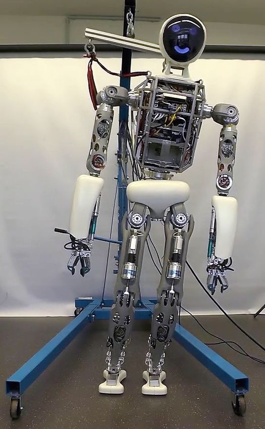
Actuator    ROM (mm)      Max. force (N)    Max. vel. (mm/s)          Joint        ROM (◦ )      Max. torque (N m)   Max. vel. (°/s)
    Wrist       235–290           495                    38           Shoulder1     −180◦ –180◦           135                210
    Torso       195–284          2716                   291           Shoulder2     −110◦ –110◦           167                131
    Hip3        272–431          4740                   175           Shoulder3     −180◦ –180◦           135                210
    Knee        273–391          5845                   140             Elbow       −125◦ –125◦           23                 413
    Ankle       221–331          2000                   265           Wrist Roll    −180◦ –180◦           18                 660
                                                                      Wrist Pitch   −46.8◦ –46.8◦        24–35              60–106
   TABLE I: ROM of linear actuators of the RH5 robot.                 Wrist Yaw     −39.6◦ –57.6◦        22–35              62–100
                                                                      Torso yaw      −40◦ –40◦             23                413
                                                                      Torso pitch    −25◦ –29◦          380–493            184–238
              Mass   Ankle      ROM           Torque      Velocity     Torso roll    −36◦ –36◦          285–386            208–400
   Robot
              (kg)   DOF         (◦ )         (Nm)         (◦ /s)        Hip1       −180◦ –180◦           135                210
                                                                         Hip2         −46◦ –67◦           135                210
                     Roll    −19.5–19.5        40             120        Hip3         −17◦ –72◦         357–540            88–133
   TORO       7.65
                     Pitch    −45–45           130            176        Knee          0◦ –88◦          337–497            94–139
                     Roll      −30–30          100            275     Ankle pitch    −51.5◦ –45◦        121–304            200–502
   TALOS      6.65                                                    Ankle roll      −57◦ –57◦         84–158             386–726
                     Pitch     −75–45          160            332
                     Roll     −57–57           84–158     386–726    TABLE III: ROM of the RH5 humanoid robot in its inde-
    RH5       3.6
                     Pitch    −51.5–45        121–304     200–502
                                                                     pendent joint space (generalized coord. when robot is fixed).
TABLE II: Comparison of lower limbs design characteristics
between the TORO, TALOS and RH5 humanoid robots.
                                                                     intersection point of the joint axes is at a height of 1800 mm
                                                                     above the foot contact area. The head weighs 3.3 kg and
design that outperforms the ankle of similar humanoid robots         includes laser scanner, stereocamera, microphones, infrared
at almost half of their weight (see Table II). Table III             camera and some processing units.
shows the ROM, speed and torque limits in the generalized               4) Arm: The robot is equipped with two manipulators.
coordinates (see [17] for a detailed analysis).                      Each manipulator includes a 3 DOF shoulder joint, an
    2) Leg: The two legs of the robot are identical in con-          1 DOF elbow, a 3 DOF wrist (realized with a rotary
struction and follow a Spherical–Revolute–Universal (SRU)            actuator in series with 2-SPU+1U mechanism) and a 1
kinematic design. Each leg has a 3 DOF hip joint (realized           DOF underactuated gripper. The intersection points of the
with 2 DOF serial mechanism and 1-RRPR mechanism),                   shoulder joint axes have a distance of 640 mm between
1 DOF knee joint (1-RRPR mechanism) and a 2 DOF                      the right and left shoulder. The first axis is tilted forward
ankle joint (2-SPRR+1U mechanism). The rotation axes of              by 14 degrees with respect to the XZ-plane of the robot
the hip joint intersect at a single point that is located at         to increase the manipulation area in front of the torso.
approximately half of the total height of the robot at 930           The lengths of the upper and lower arms are 355 mm and
mm. The distance between both hip joints is 220 mm. To               386 mm, respectively. Upper and lower arm are coupled
adjust the available range of motion, the first joint axis was       by the elbow joint. The three joint axes of the wrist also
tilted by 15 degrees with respect to the XY-plane of the robot.      form a common point of intersection. The end effector is a
The lengths of the upper and lower leg are almost identical          self-adaptive three-finger gripper, whose individual fingers
with lengths of 410 and 420 mm, respectively.. Upper and             are simultaneously actuated. The upper and lower arm
lower leg are connected by the knee joint. The ankle joint           including gripper weight 3.6 and 3.3 kg, respectively.
has two rotation axes that intersect the same point. The
axis intersection point is 100 mm above the ground contact
surface. Contact with the ground is made via 4 contact points,       B. Electronic Design and Processing Architecture
which span a support polygon with an area of 80 mm x 200                The RH5 humanoid robot uses a hybrid control approach
mm. The total mass of a leg is 9.8 kg, of which 6.2 kg are           that combines local control loops for low-level motor control
assigned to the thigh and hip joint, 2.3 kg to the lower leg,        and central controllers for high level control as depicted in
and 1.3 kg to the foot, respectively.                                Fig. 3.
    3) Torso and Head: We use a spherical body joint with               1) Decentralized Actuator-Level Controllers: In particu-
3 DOF (a 2-SPU+1U unit) to expand the body ROM, which                lar, each of the individual actuators is controlled by dedi-
translates to i) the realization of more complex walking             cated electronics placed near the actuator. On the hardware
patterns, ii) the improvement of the robot balance, and iii)         side, this modular approach facilitates the cabling effort,
a larger manipulation space. The intersection point of the           as it is sufficient to have shared power lines for digital
joint axes is at a height of 1140 mm above the foot contact          communication to the central controllers. The individual
area and it weights 4.8 kg. The body joint carries the torso,        electronics are composed of one or two motor driver boards,
which contains most of the electronics and the battery of the        a processing board based on a Xilinx Spartan 6 Field
robot and acts as a connecting structure between the robot’s         Programmable Grid Array (FPGA), and a board connecting
extremities. The torso weighs 21 kg in total. The robot also         sensors and communication lines. In addition, the hardware
has a head that serves as a sensor carrier for imaging and           structure at the control level allows decentralized low-level
acoustic perception. This includes a joint with 3 DOF. The           control, which enables local control loops with low latency.
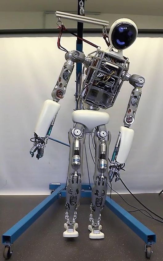
Design, analysis and control of the series-parallel hybrid RH5 humanoid robot
- Preprocessing

                                                 High-Level Control               A. Contact Stability Soft-Constrained DDP
                                                 - ROCK Framework
                                                 - Joint Drivers
                                                                                    1) Formulation of the Trajectory Optimization Problem:
                                                 - Kinematics, Dynamics, ...      Consider a system with discrete-time dynamics as
                                       er
                                 Should
                                                             Gripp
                                                                                                        x i+1 = f (x i , u i ),                    (1)
                                                     Wrist           er

                                                                                  which can be modeled as a generic function f that describes
                                              Mid-Level                           the evolution of the state x ∈ Rn from time i to i + 1, given
                      Body
                                              - Communication                     the control u ∈ Rm . The total cost J of a trajectory can
                                                                                  be written as the sum of running costs ` and a final cost
                                                                                  `f starting from the initial state x 0 and applying the control
                                 Hip             Low-Level Control                sequence u along the finite time-horizon:
                                       1D Act.
                                                 - Feedback+Feedforward Control
                                       Force     - Joint sensors handling                                                 N
                                                                                                                          X −1
                                     Knee
                                                                                             J(x 0 , u) = `f (x N ) +            `(x i , u i ).    (2)
                                                                                                                          i=0

                             Ankle                                                The cost ` at one discrete time-point (i.e., node) of the
                                                                                  optimization depends on the assigned weight αc and the
                                        6D                                        according cost term Φc as
                                        F/T

                                Contacts                                                                     C
                                                                                                             X
                                                                                                       `=          αc Φc (x , u).                  (3)
                  Fig. 3: Electronic and control units of the RH5 robot.
                                                                                                             c=1

                                                                                  Hence, we write the generic optimal control problem as
                                                                                                                  N −1 Z tk +∆t
These local controllers are implemented as a cascade of                                                           X
feedback controllers for motor current, velocity and position,                     X ∗ , U ∗ = arg min `N (xN ) +               `k (x , u)dt,
                                                                                                      X,U                        tk
                                                                                                                         k=0
which runs at frequencies of 32 KHz, 4 KHz and 1 KHz,                                                                                              (4)
respectively. Additionally, the local controllers provide feed-
forward connections to the high level controllers. This allows                                 s.t.         u ≤ u ≤ ū,                            (5)
to feed-forward velocity and motor current, therefore the                                                   ẋ = g (x , u)
amount of feedback can be locally limited to achieve a
                                                                                  where a complete trajectory X , U is a sequence of
desired compliant behavior. Note that joint position and
                                                                                  states X = {x 0 , x 1 , ..., x N } and control inputs U =
velocity can be mapped between the independent joint space
                                                                                  {u 0 , u 1 , ..., u N − 1} satisfying Eq. (1) and the system
and actuator space locally, which is also needed for the ini-
                                                                                  dynamics, and u and ū are the lower and upper torque limits
tialization of the motor’s incremental encoder position offset
                                                                                  of the system, respectively.
if the absolute position sensor measures the independent joint
                                                                                     To solve the trajectory optimization problem of Eq. (4),
position.
                                                                                  we use the Box-FDDP algorithm [13], which is publicly
    2) Central Electronics for Mid- & High-Level Control:                         available in the open-source library C ROCODDYL [18]. The
A hybrid FPGA / ARM-based system translates and routes                            Box-FDDP algorithm can compute highly-dynamics motions
status and command messages between the actuators, sensors                        thanks to its direct-indirect hybridization approach.
and a central control PC connected via an Ethernet connec-                           2) System Dynamics: The dynamics of floating base sys-
tion. In order to maximize the transmitted packets to the                         tems is given as:
central control PC while guaranteeing a an upper limit of
                                                                                                                                  k
transmission delay, we implement a routine to synchronize                                                                         X
                                                                                             M (q )v̇ + h(q , v ) = S τ +               J Tci λ,   (6)
the translation layer to the command messages. On the
                                                                                                                                  i=1
control PC, the robot middleware ROCK is used. Software
components within this framework act as drivers, which                            where M is the generalized inertia matrix, q ∈ SE(3) × Rn
handles the actuator setup and data exchange. It also pro-                        are generalized coordinates, v is the tangent vector, S is the
vides a robot-agnostic interface to the software components                       actuator selection matrix, J ci is the Jacobian at the location
implemented in the high level control. The driver components                      of a contact frame ci and w i is the contact wrench acting
run periodically at a frequency of 1 kHz, resulting in a round                    on the contact link i.
trip time of 1 ms.                                                                   3) Rigid Contact Constraints: Contacts can be expressed
                                                                                  as kinematic constraint on the equation of motion Eq. (6) as
                                                                                                        J c v̇ + J̇ c v = 0 .                      (7)
                      III. A NALYSIS AND CONTROL USING DDP
                                                                                  In order to express the holonomic contact constraint
  This section describes the trajectory optimization approach                     φ(q ) = 0 in the acceleration space, it can be differentiated
and outlines the simulation and control architecture.                             twice. Consequently, the contact condition can be seen
Design, analysis and control of the series-parallel hybrid RH5 humanoid robot
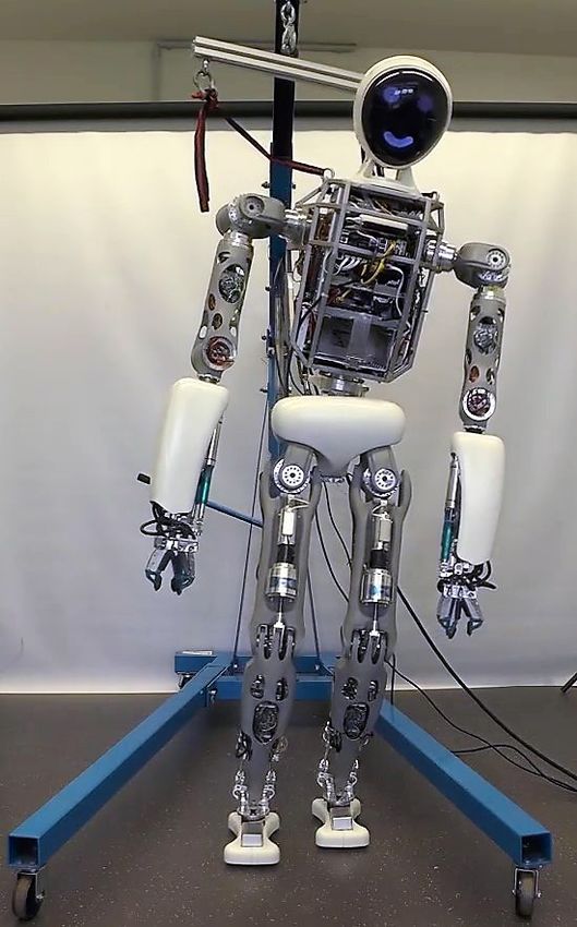
1. Offline Motion Planning
as a first order differential-algebraic equation with J c =
  J c1 · · · J ck as a stack of f contact Jacobians. Finally,                                       Whole-Body
                                                                           Contacts           Trajectory Optimization
the multi-contact dynamics can be expressed as
                                                                          Constraints
                       J>
                                          
                M       c       v̇    Sτ − h
                                    =            .                (8)
                 Jc    0       −λ      −J̇ c v
                                                                                                                                 2. Online Tracking
For more details about the hybrid optimal control (OC) using                                     Simulation Pipeline
this contact dynamics see [11].                                             Trajectory File             PD-Control
   4) Optimization Constraints: We consider constraints of                                              Architecture
the trajectory optimization problem via a cost-penalization
in Eq. (4). Cost terms can either incorporate equality or                                        Experimental Pipeline
inequality constraints, which are described in the following.
   In case of equality constraints, an arbitrary task can be                                            Joint Space         Low-Level
                                                                                                     Inverse Dynamics    Actuator Control
formulated as a quadratic regulator term as

                    Φc =|| f (t) − f ref (t) ||22 ,                              Fig. 4: Simulation and experimental pipeline.

where f (t) and f ref are actual and reference features, respec-
tively. The DDP algorithm utilizes the derivatives of these              support area:
regulator functions, namely computing the Jacobians and
Hessians of the cost functions. We use equality constraints                                               λz > 0,
for the the CoM tracking (ΦCoM ) and the tracking of the left-                                         | λx | ≤ µλz ,
and right-foot pose (Φfoot ), respectively.                                                            | λy | ≤ µλz ,                       (10)
   Equally important for physically consistent trajectory op-                                          | X | ≥ cx ,
timization is the consideration of boundaries, such as robot
limits and stability constraints. These inequality constraints                                          | Y | ≥ cy .
can be included as penalization term as well. To do so, we               In Eq. (10) µ denotes the static coefficient of friction and
use a bounded quadratic term as                                          models a spatial friction cone, and cx and cy denote the
                                                                         position of the CoP with respect to the dimensions X and Y
                             1 T
                       
                       
                              r r     | r > r > r̄                      of the rectangular robot feet. This motion planning approach
                Φc =         2                                    (9)    is what we call the contact stability soft-constrained DDP
                       
                        0             | r ≤ r ≤ r̄,                     [21].
                                                                         B. Simulation and Control Architecture
where r is the computed residual vector and r and r̄ are the
                                                                            We track the motions planned with the proposed trajectory
lower and upper bounds, respectively. In the scope of our
                                                                         optimization approach in real-time with a PD-controller
work, we define inequality constraints for joint position and
                                                                         in the PyBullet simulator and with a joint space online
velocity limits (Φjoints ), friction cone constraints (Φfriction ) and
                                                                         stabilization on the real system as depicted in Fig. 4. In the
center of pressure (ΦCoP ).
                                                                         following, details on the involved components are provided.
   Additional to the described constraints for tasks and phys-              The contact stability soft-constrained DDP approach com-
ical consistency, we optimize for minimization of the torques            putes inherently balanced motions that are concisely cap-
(Φtorques ) and regularize the robot posture (Φposture ).                tured in an appropriate file. This trajectory file contains
   5) Contact Stability: A key objective in trajectory opti-             the optimal state trajectories X ∗ , OC inputs U ∗ and the
mization for legged systems is to ensure a balanced motion               resulting contact wrenches F ∗ext acting on the feet. The
that prevents the robot from sliding and falling down. We                trajectories are interpolated to 1 kHz using cubic splines
ensure the robot stability by applying the concept of contact            in order to ensure smoothness. The planned motions are
wrench cone [19], instead of the widely accepted zero-                   computed based on a tree type robot model. For dynamic
moment point criterion [20]. Note that the latter method is              real-time control, this simplified model turns out to be suf-
limited due to the assumptions of sufficiently high friction             ficient, although the accuracy is reduced [22]. Nevertheless,
and the existence of one planar contact surface; instead, the            the problem remains on transforming the results from the
former also is suitable for multi-contact OC.                            independent joint space, to the actuation space. We use
   To this end, we model 6D surface contacts in the OC                   the modular software framework HyRoDyn (Hybrid Robot
formulation of Eq. (4) with dedicated inequality constraints             Dynamics) [23] to map the trajectories generated for the
for unilaterality of the contact forces, Coulomb friction on             serialized robot model to compute the forces of the respective
the resultant force, and center of pressure (CoP) inside the             linear actuators. Low-level actuator controllers compensate
Design, analysis and control of the series-parallel hybrid RH5 humanoid robot
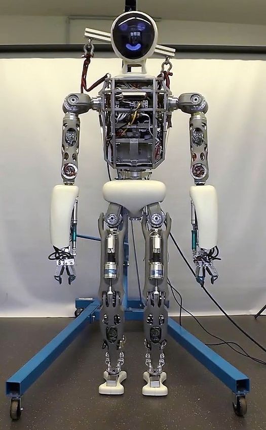
0.20                                                                                                           LF Joint Velocities [rad/s]
                       start                          end         CoM                       6
                                                                  CoMStart                                                                                           hip 1
        0.15                                                      CoMRFLiftOff              4                                                                        hip 2
                                                                  CoMRFTouchDown                                                                                     hip 3
               LF
                                                                  CoMLFLiftOff              2                                                                        knee
        0.10                                                                                                                                                         ankle roll
                                                                  CoMLFTouchDown            0
                                                                  CoMEnd                                                                                             ankle pitch
        0.05                                                      CoPLF                     2
                                                                  CoPRF                     4
Y [m]

        0.00
                                                                                            6
                                                                                                0         10      20                   30            40         50
        0.05
                                                                                          150
                                                                                                                         Torso Torques [Nm]
                                                                                                                                                                     body pitch
        0.10                                                                              100                                                                        body roll
               RF
                                                                                                                                                                     body yaw
        0.15                                                                               50
                                                                                            0
        0.20
                0.0   0.1      0.2   0.3       0.4   0.5    0.6     0.7            0.8     50
                                           X [m]
                                                                                          100

Fig. 5: Dynamic walking gait computed with the contact                                    150
                                                                                                0         10      20                   30            40         50
stability soft-constrained DDP. The motion is inherently
                                                                                         Fig. 6: Optimal solution of the dynamic walking gait with
balanced, since the CoPs (crosses) for both feet (LF, RF)
                                                                                         5 kg weights in each hand within the robot’s velocity and
remain inside the desired CoP region of 50% foot coverage
                                                                                         torque limits (dashed lines).
(dashed lines).

deviations from the reference trajectories. Analogously to
the simulation pipeline, this real-time control approach uses
a cascaded feedback of position, velocity and an additional
current control loop.

                      IV. R ESULTS AND DISCUSSIONS
  This section presents the evaluation of the robot design,
simulation results and first experimental trials.
                                                                                                    (a)                     (b)                           (c)
A. Evaluation of Robot Design                                                              Fig. 7: Squatting with 5kg aluminum bars in each hand.
   We evaluated the RH5 humanoid design by performing a
wide range of complex motions. The motivation is to form
a basis of decision-making for future design iterations that                             the OC solver found a feasible solution within the robot
allow us to perform such tasks. Table IV provides details on                             limits, proofing for the versatility of the RH5 robot design.
the performed motions and Table V summarizes the results.                                   2) Squatting with Weights: As for fast dynamic walking,
   1) Dynamic Walking Variants: We study efficient motions                               we analyzed a sequence of dynamic squatting movements
for dynamic walking gaits with high velocities. To this end,                             with a predefined CoM range of 20 cm (see Fig. 7). We also
we apply the proposed approach of contact stability soft-                                found that the joint position, velocity and torque limits were
constrained DDP, where the CoP of each foot is constrained.                              satisfied.
By this, the solver is enabled to find an optimal, dynamic                                  3) Jumping Variants: We analyzed the limits of the sys-
CoM shifting along with the requested contact stability con-                             tem design by performing highly-dynamic jumps.
straints. Fig. 5 shows this approach yields dynamically bal-                                   a) Vertical jumping: Although the RH5 robot has been
anced walking motions where the CoP of each foot (crosses)                               designed for walking motions and not highly-dynamic ones,
in contact stays within a predefined range. Following our                                vertical jumps with a height of 1 cm can be performed within
motion planning approach, we observed that often, for speeds                             valid ranges for joint position, velocity and torques. For the
greater than 0.35 m/s, the solver needs to be initialized with a                         case of a 10 cm jump the joint position and torques limits
predefined CoM trajectory in order to find a feasible solution,                          are within the limits. However, velocity peaks at the take-
as done in [11].                                                                         off exceed the limits of the body pitch and knee joints by a
      a) Walking with weights (5kg Bars): We evaluated the                               factor of two and four, respectively. This effect is plausible,
capabilities of the RH5 robot to perform a dynamic walking                               since both the knee as well as the torso swing are essential
gait at 0.35 m/s while carrying 5kg aluminum weights in each                             for a jump. We deployed a heuristic approach to identify
hand (see Fig. 1). A natural CoM shifting emerges resulting                              the minimal design improvement by scaling the critical joint
from the inequality constraints for the CoP of each foot.                                limits step by step until a feasible solution is found. For the
Fig. 6 shows that the found optimal solution is within the                               10 cm vertical jump we found that an optimal solution is
joint position and velocity limits as well as torque limits.                             found by scaling only the knee joint velocity limits of the
      b) Walking with high speed (1 m/s): In order to analyze                            robot by a factor of 3.
the limits of the RH5 humanoid, we successfully performed                                      b) Jumping over multiple obstacles: Finally, investi-
a fast dynamic walking gait at 1 m/s with a predefined CoM                               gated a more challenging jumping sequence over obstacles
trajectory (see Table IV). Also for this dynamic walking gait,                           (see Fig. 8). Since the humanoid was not designed for such
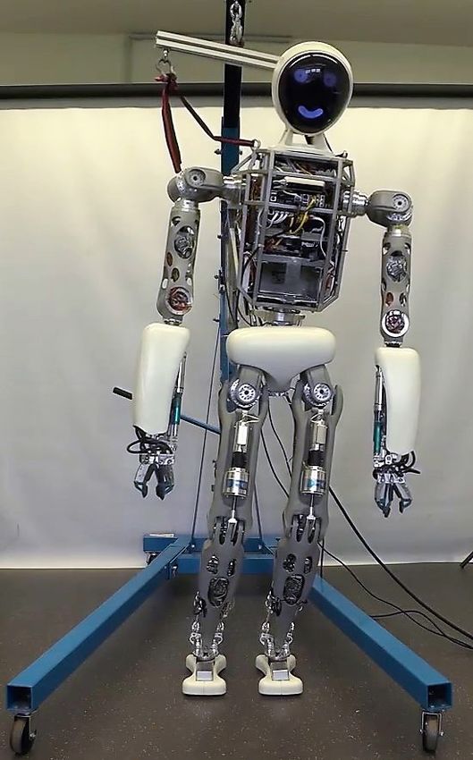
Design, analysis and control of the series-parallel hybrid RH5 humanoid robot
(a)                             (b)                          (c)                                                         (d)                                    (e)
                                                                                       Fig. 10: Experiment I: one-leg balancing from (a) an initial
                          (a)                               (b)                        pose, (b) CoM shift above the LF, (c) lifting the RF up and
           Fig. 8: Sequence of challenging jumps over obstacles.                       (d) down and (e) recovering to the initial pose.

                0.4                                                      des
                0.3                                                      act
        X [m]

                0.2
                0.1
                0.0

         0.050
         0.025
Y [m]

         0.000
         0.025
         0.050

           0.92                                                                                                                     (a)                             (b)                          (c)                                                         (d)                                    (e)
           0.91
   Z [m]

           0.90                                                                        Fig. 11: Experiment II: static stepping motion from (a) an
           0.89
           0.88                                                                        initial pose, (b) CoM shift above the LF, (c,d) performing a
                      0    1000   2000            3000   4000     5000
                                         t [ms]                                        right step and (e) shifting the CoM to the center of the SP.
Fig. 9: Motion of the floating base resulting from joint level
control for the dynamic walking gait.
                                                                                       Fig. 13) involves dynamic forces acting on the robot resulting
                                                                                       from a fast vertical base movement in the range of 15 cm
tasks, neither joint velocity nor torque limits can be satisfied.                      within two seconds. Overall, the three planned motions could
Further details on the formulation of the OC problems,                                 be stabilized with good accuracy by the controller on the
used optimization constraints, extracted design guidelines                             real system. Fig. 12 shows the tracking performance for
and videos are provided in [21].                                                       the one-leg balancing experiment. The control architecture
                                                                                       allows following the computed reference trajectory closely,
B. Simulation Results                                                                  both in actuator space (a,b) and independent joint space
  We proved the stability of the optimized dynamic walking                             (c,d). This precise tracking is achieved with high-gain joint
motion in the PyBullet simulator using a joint space PD                                space control, which allows a quick compensation of position
controller. Fig. 9 monitors the optimized motion of the                                differences that comes at the cost of lost compliance in the
uncontrolled floating base. As can be seen, the floating base                          joints. The impact phase turned out to be the main problem
deviates about ± 10 mm in x- and y-direction as well                                   for the walking experiments. This is reasonable since the
as + 5 mm in z-direction. The motions turn out to be                                   utilized control approach only compensates for errors in joint
inherently balanced due to the proposed contact stability soft-                        space, while errors in task space can arise quickly and are
constrained DDP approach. Hence, our trajectories did not                              not compensated.
                                                                                                                           Date: Friday, August 28, 2020 11:59:25, Joint: LLAnkle_Act1                                                   Date: Friday, August 28, 2020 11:59:25, Joint: LLAnkle_Act2
require a dedicated online stabilizer, in contrast to the work
of [14], to generate a physically consistent motion.                                                                                                  Joint Position
                                                                                                                                                                                                                                0.0245
                                                                                                                                                                                                                                                                    Joint Position
                                                                                                                   0.022
                                                                                                                                                                                                                                0.0240
                                                                                                                   0.020                                                                                                        0.0235
C. Experimental Trials
                                                                                     Position [rad]

                                                                                                                                                                                                   Position [rad]

                                                                                                                                                                                                                                0.0230
                                                                                                                   0.018
                                                                                                                                                                                                                                0.0225
                                                                                                                   0.016                                                                                                        0.0220
   We conducted three experiments with increasing level of                                                         0.014
                                                                                                                                                                                                                                0.0215
                                                                                                                                                                                                                                0.0210
difficulty. The goal of the first experiment is to test the ability                                                         Date: Friday, August 28, 2020 11:59:34, Joint: LLAnkleRoll
                                                                                                                                                      Joint Speed
                                                                                                                                                                                                                                         Date: Friday, August 28, 2020 11:59:34, Joint: LLAnklePitch
                                                                                                                                                                                                                                                                    Joint Speed
                                                                                                                                                                                                                                      0.025
of the controller to track a slow balancing task. The quasi-                                                       0.005                  (a) LLAnkleAct1
                                                                                                                                                Joint Position                                                                        0.020           (b) LLAnkleAct2
                                                                                                                                                                                                                                                            Joint Position
                                                                                                                   0.000                                                                                                              0.015
                                                                                                                    0.14                                                                                                               0.24
                                                                                      Joint Speed [rad/s]

                                                                                                                                                                                                               Speed [rad/s]

static motion consists of five phases as visualized in Fig. 10.                                                     0.12
                                                                                                                   0.005
                                                                                                                                                                                                                                      0.010
                                                                                                                                                                                                                                       0.25
                                                                                                                                                                                                                                      0.005
                                                                                                                    0.10                                                                                                               0.26
The second experiment deals with a stabilization of a static                                                       0.010                                                                                                              0.000
                                                                               Position [rad]

                                                                                                                                                                                                           [rad]
                                                                                                                                                                                                 PositionJoint

                                                                                                                    0.08                                                                                                              0.005
                                                                                                                   0.015                                                                                                               0.27
                                                                                                                    0.06                                                                                                              0.010
stepping motion (see Fig. 11). The objective of this test is                                                        0.04
                                                                                                                   0.020
                                                                                                                    0.02                                 Time [s]
                                                                                                                                                                                                                                       0.28
                                                                                                                                                                                                                                      0.015
                                                                                                                                                                                                                                       0.29                            Time [s]
                                                                                                                                                   Joint Force/Torque                                                                                           Joint Force/Torque
to analyze the effect of more difficult swing-leg motions, a                                                        0.00
                                                                                                                     200
                                                                                                                                                                                                                                      0.30
                                                                                                                                                                                                                                       200
                                                                                                                                                      Joint Speed                                                                        0                          Joint Speed
                                                                                                    [N] or Torque [Nm]

                                                                                                                                                                                                                 [N] or Torque [Nm]

step sequence of two steps and the effect of impacts. The                                                                  0
                                                                                                                         0.2              (c) LLAnkleRoll                                                                             0.10
                                                                                                                                                                                                                                       200
                                                                                                                                                                                                                                                      (d) LLAnklePitch
                                                                                                                         200                                                                                                           400
objective of the third experiment is to evaluate the tracking                                                                                                                                                                         0.05
                                                                                                                                                                                                                                       600
                                                                                              Force [rad/s]

                                                                                                                                                                                                           Force [rad/s]

                                                                                                                         0.1
                                                                                                                         400
                                                                                                                                                                                                                                       800
                                                                                       Fig. 12: Tracking performance for the one-leg balancing                                                                                        0.00
                                                                                       Joint Speed

                                                                                                                                                                                                    Joint Speed

                                                                                                                         600                                                                                                          1000
performance in the context of a dynamic motion. In contrast                                                              0.0
                                                                                                                         800                                                                                                          1200
                                                                                                                                                                                                                                      0.05

to the first two motions, the fast squatting experiment (see                           experiment in actuators (a,b) and independent joints (c,d).
                                                                                                                         0.1
                                                                                                                                0           10          20
                                                                                                                                                        Time [s]
                                                                                                                                                                            30         40
                                                                                                                                                                                                                                      1400
                                                                                                                                                                                                                                       0.10
                                                                                                                                                                                                                                              0         10            20
                                                                                                                                                                                                                                                                      Time [s]
                                                                                                                                                                                                                                                                                          30           40
                                                                                                                          0.2
                                                                                                                                                         Time [s]                                                                                                      Time [s]
                                                                                                                                                   Joint Force/Torque                                                                                           Joint Force/Torque
                                                                                                                         0.04                                                                                                          0.04
                                                                                   Force [N] or Torque [Nm]

                                                                                                                                                                                                        Force [N] or Torque [Nm]

                                                                                                                         0.02                                                                                                          0.02

                                                                                                                         0.00                                                                                                          0.00

                                                                                                                         0.02                                                                                                          0.02

                                                                                                                         0.04                                                                                                          0.04

                                                                                                                                     0      5    10        15          20        25   30    35                                                    0     5      10        15          20        25     30    35
Design, analysis and control of the series-parallel hybrid RH5 humanoid robot
TABLE IV: Characteristics and applied optimization constraints for a wide range of dynamic motions.
                                                    Motion Characteristics                                    Optimization Constraints
                                           Length   Height   Total time    Step size           Tasks             Stability    Limits    Regularization
                                                                                           Φfoot   ΦCoM      Φfriction   ΦCoP Φjoint   Φposture  Φtorque
 Dynamic walking with 5kg weights          0.5 m     0.05 m        1.5 s        0.03   s    5                  5           5    5        5          5
 Fast dynamic walking (1 m/s)              0.7 m      0.1 m        0.7 s        0.03   s    5        5                          5        5          5
 Squatting with 5kg weights                  –        0.2 m         2s          0.03   s    5        5         5           5    5        5          5
 Vertical jump (h = 0.01 m)                  –       0.01 m        0.9 s        0.01   s    5                  5           5    5        5          5
 Vertical jump (h = 0.1 m)                   –        0.1 m        0.9 s        0.01   s    5                  5           5    5        5          5
 Jumps over obstacles                      0.6 m     0.25 m        2.7 s        0.01   s    5                  5           5    5                   5

TABLE V: Capabilities of the RH5 humanoid to perform a                            [5] N. A. Radford, P. Strawser, K. Hambuchen, J. Mehling, and et. al.,
wide range of motions respecting the hardware limits.                                 “Valkyrie: Nasa’s first bipedal humanoid robot,” Journal of Field
                                                                                      Robotics, vol. 32, no. 3, pp. 397–419, 2015.
 Experiment                       Pos. Lim.     Torque Lim.     Vel. Lim.         [6] J. Englsberger, A. Werner, C. Ott, B. Henze, M. A. Roa, G. Garo-
 Walk with 5kg weights               X               X              X                 falo, R. Burger, A. Beyer, O. Eiberger, K. Schmid, and A. Albu-
 Dynamic walk (1 m/s)                X               X              X                 Schäffer, “Overview of the torque-controlled humanoid robot toro,”
 Squats with 5kg weights             X               X              X                 in Humanoids, 2014.
 Vertical jump (h = 0.01 m)          X               X              X             [7] O. Stasse, T. Flayols, and et. al., “Talos: A new humanoid research
 Vertical jump (h = 0.1 m)           X               X             53                 platform targeted for industrial applications,” in Humanoids, 2017.
 Forward obstacle jumps              X              55             57             [8] J. Carpentier, S. Tonneau, M. Naveau, O. Stasse, and N. Mansard,
                                                                                      “A versatile and efficient pattern generator for generalized legged
                                                                                      locomotion,” in ICRA. IEEE, 2016.
                                                                                  [9] B. Aceituno-Cabezas, C. Mastalli, H. Dai, M. Focchi, A. Radulescu,
                                                                                      D. G. Caldwell, J. Cappelletto, J. C. Grieco, G. Fernández-López, and
                                                                                      C. Semini, “Simultaneous contact, gait, and motion planning for robust
                                                                                      multilegged locomotion via mixed-integer convex optimization,” RA-L,
                                                                                      vol. 3, no. 3, pp. 2531–2538, 2017.
                                                                                 [10] S. Fahmi, C. Mastalli, M. Focchi, and C. Semini, “Passive whole-body
                                                                                      control for quadruped robots: Experimental validation over challenging
                                                                                      terrain,” RA-L, vol. 4, no. 3, pp. 2553–2560, 2019.
      (a)            (b)             (c)             (d)             (e)         [11] R. Budhiraja, J. Carpentier, C. Mastalli, and N. Mansard, “Differential
                                                                                      dynamic programming for multi-phase rigid contact dynamics,” in
Fig. 13: Experiment III: sequence of fast squats from (a) an                          Humanoids. IEEE, 2018.
                                                                                 [12] D. Mayne, “A second-order gradient method for determining optimal
initial pose over, (b,d,f) descending the CoM by 15 cm and                            trajectories of non-linear discrete-time systems,” International Journal
(c,e,g) recovering to the initial pose.                                               of Control, vol. 3, no. 1, pp. 85–95, jan 1966.
                                                                                 [13] C. Mastalli, W. Merkt, J. Marti-Saumell, H. Ferrolho, , J. Sola,
                                                                                      N. Mansard, and S. Vijayakumar, “A direct-indirect hybridization
                                                                                      approach to control-limited ddp,” arXiv:2010.00411, 2021.
                           V. C ONCLUSION                                        [14] K. Giraud-Esclasse, P. Fernbach, G. Buondonno, C. Mastalli, and
                                                                                      O. Stasse, “Motion planning with multi-contact and visual servoing
   This paper presented the design and analysis of a novel                            on humanoid robots,” in SII). IEEE, 2020.
                                                                                 [15] A. B. Zoss, H. Kazerooni, and A. Chu, “Biomechanical design
series–parallel hybrid humanoid robot named RH5 which has                             of the berkeley lower extremity exoskeleton (bleex),” IEEE/ASME
a lightweight design and good dynamic characteristics. We                             Transactions on Mechatronics, vol. 11, no. 2, pp. 128–138, April 2006.
see large potential in using DDP-based whole-body TO to                          [16] S. Kumar, A. Nayak, H. Peters, C. Schulz, A. Müller, and F. Kirchner,
                                                                                      “Kinematic analysis of a novel parallel 2sprr+1u ankle mechanism in
evaluate the capabilities of humanoid robots. The preliminary                         humanoid robot,” in Advances in Robot Kinematics 2018, J. Lenarcic
experiments indicate that the proposed planning approach                              and V. Parenti-Castelli, Eds., 2019, pp. 431–439.
efficiently generates physically consistent motions for the                      [17] S. Kumar, “Modular and analytical methods for solving kinematics
                                                                                      and dynamics of series-parallel hybrid robots,” Ph.D. dissertation,
RH5 humanoid robot. Future work includes experiments with                             Universität Bremen, 2019.
online stabilization to realize heavy-duty tasks with the real                   [18] C. Mastalli, R. Budhiraja, W. Merkt, G. Saurel, B. Hammoud,
system. We also plan to address the resolution of internal                            M. Naveau, J. Carpentier, S. Vijayakumar, and N. Mansard, “Crocod-
                                                                                      dyl: An Efficient and Versatile Framework for Multi-Contact Optimal
closed loops along with the holonomic constraints imposed                             Control,” in ICRA, 2020.
by the contacts within the DDP formulation.                                      [19] S. Caron, Q.-C. Pham, and Y. Nakamura, “Stability of surface contacts
                                                                                      for humanoid robots: Closed-form formulae of the contact wrench
                                                                                      cone for rectangular support areas,” in ICRA. IEEE, 2015.
                             R EFERENCES                                         [20] M. Vukobratović and J. Stepanenko, “On the stability of anthropomor-
                                                                                      phic systems,” Mathematical biosciences, vol. 15, no. 1-2, 1972.
 [1] O. Stasse and T. Flayols, An Overview of Humanoid Robots Technolo-          [21] J. Esser, “Highly-dynamic movements of a humanoid robot using
     gies. Cham: Springer International Publishing, 2019, pp. 281–310.                whole-body trajectory optimization,” Master’s thesis, University of
 [2] S. Kumar, H. Wöhrle, J. de Gea Fernández, A. Müller, and F. Kirchner,         Duisburg-Essen, Nov 2020.
     “A survey on modularity and distributivity in series-parallel hybrid        [22] S. Kumar, J. Martensen, A. Mueller, and F. Kirchner, “Model simplifi-
     robots,” Mechatronics, vol. 68, p. 102367, 2020.                                 cation for dynamic control of series-parallel hybrid robots-a represen-
 [3] S. Lohmeier, T. Buschmann, H. Ulbrich, and F. Pfeiffer, “Modular                 tative study on the effects of neglected dynamics,” in IROS. IEEE,
     joint design for performance enhanced humanoid robot lola,” in ICRA,             2019.
     2006.                                                                       [23] S. Kumar, K. A. v. Szadkowski, A. Mueller, and F. Kirchner, “An
 [4] J. Lemburg, J. de Gea Fernández, M. Eich, D. Mronga, P. Kampmann,               analytical and modular software workbench for solving kinematics and
     A. Vogt, A. Aggarwal, Y. Shi, and F. Kirchner, “Aila - design of an              dynamics of series-parallel hybrid robots,” Journal of Mechanisms and
     autonomous mobile dual-arm robot,” in ICRA, 2011.                                Robotics, vol. 12, no. 2, 2020.
Design, analysis and control of the series-parallel hybrid RH5 humanoid robot Design, analysis and control of the series-parallel hybrid RH5 humanoid robot
You can also read