Detecting minimoons in the Earth- Moon system with microsatellite compatible technologies - KTH
←
→
Page content transcription
If your browser does not render page correctly, please read the page content below
DEGREE PROJECT IN COMPUTER SCIENCE AND ENGINEERING,
SECOND CYCLE, 30 CREDITS
STOCKHOLM, SWEDEN 2018

Detecting minimoons in the Earth-
Moon system with microsatellite
compatible technologies

MATIAS KIDRON

KTH ROYAL INSTITUTE OF TECHNOLOGY
SCHOOL OF ELECTRICAL ENGINEERING AND COMPUTER SCIENCE
Detecting minimoons in the Earth-Moon system
  with microsatellite compatible technologies

                           November 23, 2018

                        Author: Matias Kidron

                      Supervisor: Nickolay Ivchenko
                       Examiner: Tomas Karlsson

              EF233X Degree Project in Space Technology

  A thesis submitted in fulfillment of the requirements for the degree of
                  Master in Aerospace Engineering
            in the Department of Space and Plasma Physics
         School of Electrical Engineering and Computer Science
                   KTH Royal Institute of Technology
Abstract

Minimoons, Earth’s temporarily-captured orbiters, are excellent candidates for asteroid
mining technology demonstrations and general asteroid studies because of their relatively
long stay in the vicinity of Earth. In this thesis, microsatellite compatible surveillance
technologies are discussed and the suitability of various locations in the Earth-Moon sys-
tem for minimoon surveillance is examined. This is done to acquire knowledge on which
type of an orbit a minimoon-surveying-microsatellite could be placed on.
    The instantaneous visible fraction of the minimoon steady-state population is the figure
of merit when comparing surveillance systems and locations. The visible fraction is esti-
mated by simulating the distribution of visible minimoons in the sky-plane. The objects
in the simulated sky-plane are synthetic minimoons, which are generated in large numbers
according to the geocentric 6-dimensional-residence-time-distribution of minimoons, and
thus, the bin values of the sky-plane distribution can be thought of as instantaneous prob-
abilities for containing a detectable minimoon within certain ecliptic latitude-longitude
range.
    The visible fractions are estimated for various locations with given surveillance system
performance. Multiple microsatellite compatible surveillance technology configurations
are examined as well as the e↵ect of limiting magnitude and maximum angular velocity.
Minimoons are faint and fast moving objects and thus the use of synthetic tracking algo-
rithm is beneficial and considered. Only visual band surveillance systems with aperture
sizes less than 0.30 m and minimoons with diameter sizes larger than 0.50 m are considered
in the simulations.

                                             i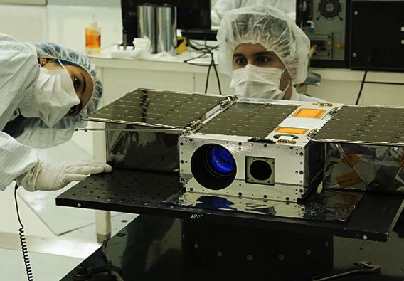
Sammanfattning

Minimånar, jordens temporärt fångade satelliter, är utmärkta kandidater för demonstra-
tioner av asteroidbrytningteknologi och för allmänna asteroidstudier på grund av deras rel-
ativt långa vistelse i närheten av jorden. I den här avhandlingen, diskuteras mikrosatellit
kompatibla övervakningsteknologier och därtill undersökes lämpligheten av olika platser
i jord-måne-systemet för övervakning av minimånar. Det här görs för att ska↵a kunskap
om vilken typ av omloppsbana en mikrosatellit för minimåneövervakning kunde placeras
på.
     Den momentana synliga fraktionen av den jämviktstillstånd minimånepopulationen är
den merit som används vid jämförelse av övervakningssystem och platser i rymden. Den
synliga fraktionen uppskattas genom att simulera fördelningen av synliga minimånar i
skyplanet. Föremålen i det simulerade skyplanet är syntetiska minimånar, vilka gener-
eras i stort antal enligt den geocentriska 6-dimensionella-uppehållstid-distributionen av
minimånarna, och sålunda kan värdena i den diskretiserade skyplanfördelningen betrak-
tas som momentana sannolikheter för att innehålla en observerbar minimåne inom det
specifiserade ecliptiska latitudinella-longitudinella området.
     De synliga fraktionerna beräknas för olika platser med det givna övervakningssys-
temets parametrar. Flera mikrosatellit-kompatibla övervakningsteknologikonfigurationer
undersöks, såväl som e↵ekterna av begränsande magnitud och maximal vinkelhastighet.
Minimånar är dunkla och snabba rörliga föremål, och således är användningen av synthetic
tracking fördelaktig och övervägd. Endast övervakningssystem som fungerar i visuellt band
med en bländarstorlek mindre än 0,30 m och minimånar med en diameter större än 0,50
m beaktas i simuleringarna.

                                               ii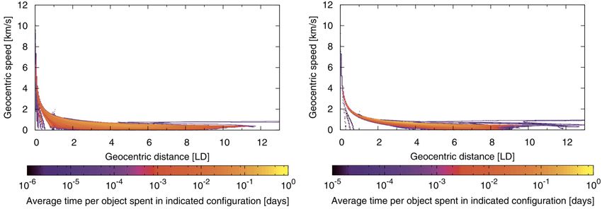
Acknowledgements

I have had amazing and inspiring teachers since the very first grade in the elementary
school. Thank you. I would especially like to thank Mikael Granvik and Grigori Fedorets
for their scientific advice and help during this thesis project. In addition, I would like to
thank my family, girlfriend, LTU and KTH for their support.

                                             iii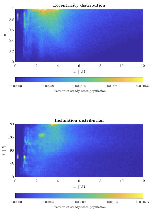
Contents

Abstract                                                                                                                                    i

Acknowledgements                                                                                                                          iii

Contents                                                                                                                                  iv

List of Figures                                                                                                                           vi

List of Tables                                                                                                                           vii

Nomenclature                                                                                                                             viii

1 Introduction                                                                                                                             1

2 Theory                                                                                                                                   3
  2.1 Brightness of objects . . .    . . . . . . .   .   .   .   .   .   .   .   .   .   .   .   .   .   .   .   .   .   .   .   .   .     3
  2.2 Cameras and telescopes .       . . . . . . .   .   .   .   .   .   .   .   .   .   .   .   .   .   .   .   .   .   .   .   .   .     5
  2.3 Detection and tracking . .     . . . . . . .   .   .   .   .   .   .   .   .   .   .   .   .   .   .   .   .   .   .   .   .   .     9
  2.4 Shift-and-add technique .      . . . . . . .   .   .   .   .   .   .   .   .   .   .   .   .   .   .   .   .   .   .   .   .   .    11
  2.5 Advantages of space-based      surveillance    .   .   .   .   .   .   .   .   .   .   .   .   .   .   .   .   .   .   .   .   .    13

3 Earth’s temporarily-captured natural satellites                                                                                         15
  3.1 Definitions . . . . . . . . . . . . . . . . . . . . . . . .                    .   .   .   .   .   .   .   .   .   .   .   .   .    15
  3.2 The creation of the population model . . . . . . . . .                         .   .   .   .   .   .   .   .   .   .   .   .   .    16
  3.3 Steady-state population . . . . . . . . . . . . . . . .                        .   .   .   .   .   .   .   .   .   .   .   .   .    16
  3.4 Earlier 6D-geocentric-residence-time-distribution . .                          .   .   .   .   .   .   .   .   .   .   .   .   .    17
  3.5 Sky-plane distributions . . . . . . . . . . . . . . . . .                      .   .   .   .   .   .   .   .   .   .   .   .   .    18
  3.6 Rate-of-motion . . . . . . . . . . . . . . . . . . . . .                       .   .   .   .   .   .   .   .   .   .   .   .   .    19
  3.7 Rotation rates . . . . . . . . . . . . . . . . . . . . . .                     .   .   .   .   .   .   .   .   .   .   .   .   .    20
  3.8 Summary of the observational challenges with TCAs                              .   .   .   .   .   .   .   .   .   .   .   .   .    20

4 MicroSat asteroid surveillance technologies                                                                                             21
  4.1 Earlier and proposed missions . . . . . . . . . .                  .   .   .   .   .   .   .   .   .   .   .   .   .   .   .   .    21
  4.2 Other available and researched technologies . .                    .   .   .   .   .   .   .   .   .   .   .   .   .   .   .   .    25
      4.2.1 Telescope technologies . . . . . . . . . .                   .   .   .   .   .   .   .   .   .   .   .   .   .   .   .   .    25
      4.2.2 Sensor technologies . . . . . . . . . . . .                  .   .   .   .   .   .   .   .   .   .   .   .   .   .   .   .    27
      4.2.3 Other technologies . . . . . . . . . . . .                   .   .   .   .   .   .   .   .   .   .   .   .   .   .   .   .    27
  4.3 Alternatives . . . . . . . . . . . . . . . . . . . .               .   .   .   .   .   .   .   .   .   .   .   .   .   .   .   .    27
  4.4 Summary of MicroSat compatible technologies                        .   .   .   .   .   .   .   .   .   .   .   .   .   .   .   .    28

                                             iv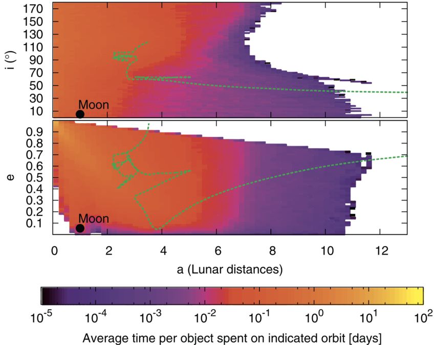
5 Simulation                                                                                                                       29
  5.1 6D-geocentric-residence-time-distribution . . . . . . . . . . . . .                                  .   .   .   .   .   .   30
  5.2 Scaled-up minimoon population . . . . . . . . . . . . . . . . . . .                                  .   .   .   .   .   .   31
  5.3 Observatories . . . . . . . . . . . . . . . . . . . . . . . . . . . . .                              .   .   .   .   .   .   34
  5.4 Observations . . . . . . . . . . . . . . . . . . . . . . . . . . . . .                               .   .   .   .   .   .   35
  5.5 Post-processing . . . . . . . . . . . . . . . . . . . . . . . . . . . .                              .   .   .   .   .   .   36
      5.5.1 The e↵ects of Earth and the Moon on observing . . . . .                                        .   .   .   .   .   .   36
      5.5.2 Examined surveillance system cases and their parameters                                        .   .   .   .   .   .   36

6 Results                                                                                                                          38
  6.1 Case S17 . . . . . . . . . . . . . . . . . . .   .   .   .   .   .   .   .   .   .   .   .   .   .   .   .   .   .   .   .   39
  6.2 Case S18 . . . . . . . . . . . . . . . . . . .   .   .   .   .   .   .   .   .   .   .   .   .   .   .   .   .   .   .   .   40
  6.3 Case NS . . . . . . . . . . . . . . . . . . .    .   .   .   .   .   .   .   .   .   .   .   .   .   .   .   .   .   .   .   45
  6.4 Case TS . . . . . . . . . . . . . . . . . . .    .   .   .   .   .   .   .   .   .   .   .   .   .   .   .   .   .   .   .   46
  6.5 General comments on the examined cases           .   .   .   .   .   .   .   .   .   .   .   .   .   .   .   .   .   .   .   47
  6.6 Performance on speculated orbits . . . . .       .   .   .   .   .   .   .   .   .   .   .   .   .   .   .   .   .   .   .   48
  6.7 Summary of results . . . . . . . . . . . . .     .   .   .   .   .   .   .   .   .   .   .   .   .   .   .   .   .   .   .   52

7 Discussion                                                                                                                       53

8 Conclusions                                                                                                                      54

Bibliography                                                                                                                       55

Appendices                                                                                60
  A   Observatory-file format . . . . . . . . . . . . . . . . . . . . . . . . . . . . . 60
  B   Objects-file format . . . . . . . . . . . . . . . . . . . . . . . . . . . . . . . . 60

                                             v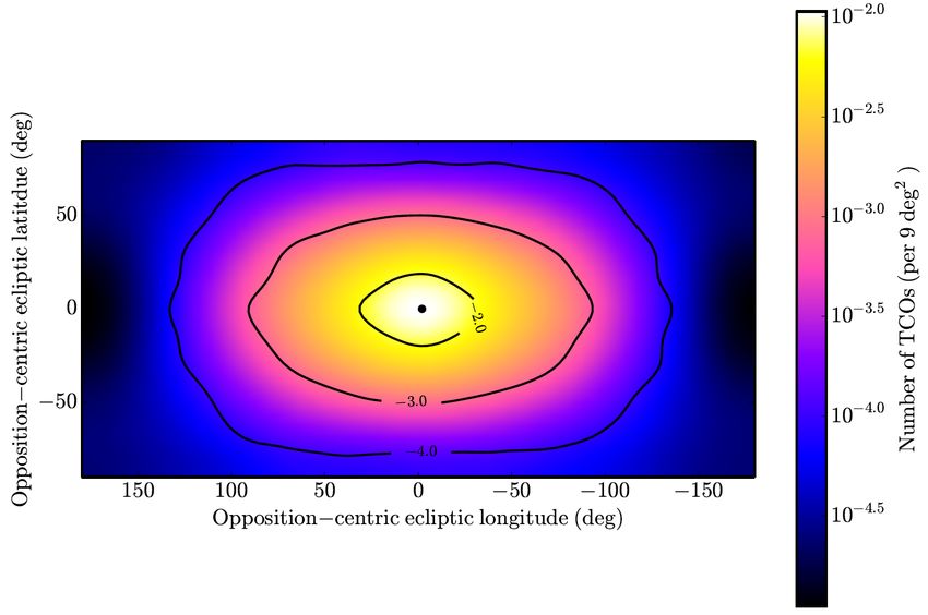
List of Figures
2.1 Definition of phase- and solar elongation angle. . . . . . . . . . . . . . . . . 4
2.2 Airy pattern. . . . . . . . . . . . . . . . . . . . . . . . . . . . . . . . . . . . 7
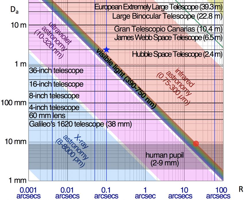
2.3 Angular resolution as a function of aperture diameter and wavelength. . . . 8
2.4 Decreasing minimoon orbit uncertainty with more observations. . . . . . . . 10
2.5 Shift-and-add technique. . . . . . . . . . . . . . . . . . . . . . . . . . . . . . 11
2.6 Computational load of synthetic tracking. . . . . . . . . . . . . . . . . . . . 12
2.7 The improvement in the peak signal with synthetic tracking. . . . . . . . . 13
2.8 Atmospheric electromagnetic opacity as a function of wavelength. . . . . . . 14
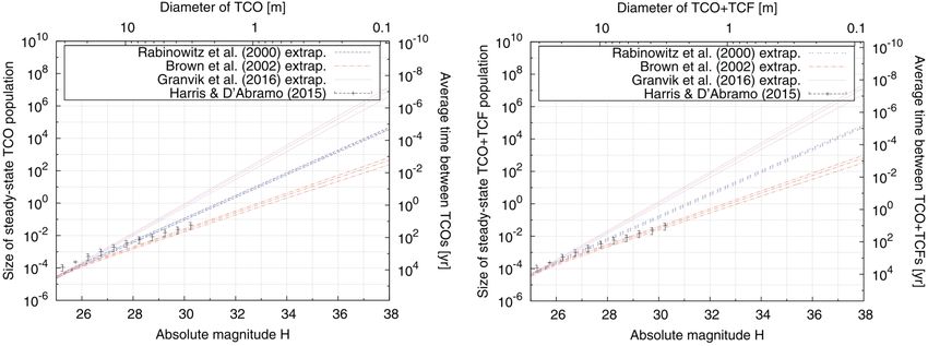
3.1 Size of the TCO and TCA steady-state populations as a function of absolute
magnitude. . . . . . . . . . . . . . . . . . . . . . . . . . . . . . . . . . . . . 17
3.2 a, e, i-residence-time distribution of minimoons. . . . . . . . . . . . . . . . . 18
3.3 Constrained sky-plane distribution of minimoons from Earth. . . . . . . . . 19
3.4 Geocentric velocities of TCAs. . . . . . . . . . . . . . . . . . . . . . . . . . 19
3.5 Rotation rates of small asteroids. . . . . . . . . . . . . . . . . . . . . . . . . 20
4.1 Computer rendering of NEOSSat. . . . . . . . . . . . . . . . . . . . . . . . . 22
4.2 ASTERIA prior to launch. . . . . . . . . . . . . . . . . . . . . . . . . . . . . 22
4.3 A CAD model of a synthetic tracking telescope. . . . . . . . . . . . . . . . . 23
4.4 Deployable optics design. . . . . . . . . . . . . . . . . . . . . . . . . . . . . 26
4.5 SpaceFab’s Waypoint MicroSat. . . . . . . . . . . . . . . . . . . . . . . . . . 26
5.1 Absolute magnitude distribution of synthetic minimoon population. . . . . 31
5.2 Distribution of minimoons in (a, e, i)-orbital element phase space. . . . . . . 32
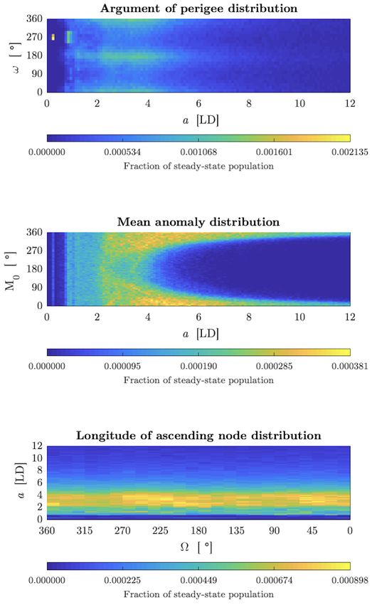
5.3 Distribution of minimoons in (!, M0 , ⌦, a)-orbital element phase space. . . . 33
5.4 Observatory locations. . . . . . . . . . . . . . . . . . . . . . . . . . . . . . . 35
6.1 Case S17: Sky-plane distribution at highest vf location. . . . . . . . . . . . 40
6.2 Case S18: Visible fractions at observatory locations. . . . . . . . . . . . . . 41
6.3 Case S18: The sky-plane distribution at highest vf location. . . . . . . . . . 42
6.4 Case S18: The sky-plane distribution of angular velocity at highest vf d
location. . . . . . . . . . . . . . . . . . . . . . . . . . . . . . . . . . . . . . . 42
6.5 Case S18 with decreased velocity search range at di↵erent observatory lo-
cations. . . . . . . . . . . . . . . . . . . . . . . . . . . . . . . . . . . . . . . 44
6.6 Case S18: x- and y-coordinates of visible synthetic minimoons. . . . . . . . 45
6.7 Case TS: The sky-plane distribution at highest vf location. . . . . . . . . . 47
6.8 Case S18: Earth’s decreasing e↵ect on visible fraction. . . . . . . . . . . . . 48
6.9 Limiting magnitude as a function of aperture diameter. . . . . . . . . . . . 50
6.10 Visible fraction as a function of limiting magnitude at speculated orbits. . . 50
6.11 Visible fraction as a function of maximum angular velocity at speculated
orbits. . . . . . . . . . . . . . . . . . . . . . . . . . . . . . . . . . . . . . . . 51
6.12 Distribution of vf in the EMS with less capable S18. . . . . . . . . . . . . . 51
vi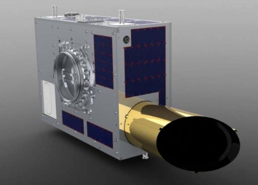
List of Tables

 2.1   Values of basis functions. . . . . . . . . . . . . . . . . . . . . . . . . . . . .                        5
 2.2   Geometric albedos and G1 and G2 constants for three main asteroid types.                                  5

 4.1   The parameters used in Shao et al. (2017) to estimate system performance.                                 23

 5.1   Bin widths and ranges used in the 6DGRTD. . . . . . . . . . . . . . . . . . 30
 5.2   Observatory coordinates. . . . . . . . . . . . . . . . . . . . . . . . . . . . . . 34
 5.3   Surveillance system parameters used in test cases. . . . . . . . . . . . . . . 37

 6.1   S17 results. . . . . . . . . . . . . . . . . . . . . . . . . . . .    .   .   .   .   .   .   .   .   .   39
 6.2   S18 results. . . . . . . . . . . . . . . . . . . . . . . . . . . .    .   .   .   .   .   .   .   .   .   41
 6.3   NS results. . . . . . . . . . . . . . . . . . . . . . . . . . . .     .   .   .   .   .   .   .   .   .   46
 6.4   TS results. . . . . . . . . . . . . . . . . . . . . . . . . . . . .   .   .   .   .   .   .   .   .   .   46
 6.5   Case S18: Averaged results for speculated spacecraft orbits.          .   .   .   .   .   .   .   .   .   49
 6.6   Results summary for cases. . . . . . . . . . . . . . . . . . .        .   .   .   .   .   .   .   .   .   52

 A.1 .gaia3 format. . . . . . . . . . . . . . . . . . . . . . . . . . . . . . . . . . . . 61
 B.1 .des format. . . . . . . . . . . . . . . . . . . . . . . . . . . . . . . . . . . . . 62

                                             vii
Nomenclature
Acronyms
6DGRTD 6-dimensional-geocentric-residence-time-distribution
ASTERIA Arcsecond Space Telescope Enabling Research in Astrophysics
CANYVAL-X CubeSat Astronomy by NASA and Yonsei using Virtual Telescope Align-
ment eXperiment
CCD Charge-coupled-device
CDST Collapsible-tube Deployable Space Telescope
CMOS Complementary metal–oxide–semiconductor
COTS Commercial-o↵-the-shelf
DPT Deployable Petal Telescope
EMS Earth-Moon system
FPGA Field programmable gate array
GEO Geosynchronous equatorial orbit
GPU Graphics Processing Unit
HSC Hyper Suprime-Cam
L Lagrange point
LEO Low Earth orbit
LSST Large Synoptic Survey Telescope
NEA Near-Earth asteroid
NEO Near-Earth object
NEOSSat Near Earth Object Surveillance Satellite
NES Natural Earth satellite
PHO Potentially hazardous object
TCA Temporarily-captured-asteroid
TCF Temporarily-captured-flyby
TCO Temporarily-captured-orbiter
viiiSymbols
↵ Phase angle
e Ecliptic longitude
v Delta-v
Asteroid to observer distance
✏ Obscuration factor
⌘ Specific energy
Solar elongation
Wavelength
e Ecliptic latitude
µ Standard gravitational parameter
DC Dark current
Heliocentric - used as a sub-index
⌦ Longitude of ascending node
! Argument of perihelion
!r Rate of rotation
Phase function
⌧ Transmittance
⇥ Di↵raction limited angular resolution
✓ Angle away from the Sun in the ecliptic
⇣ Topocentric angular velocity
a Semi-major axis
C Computational load
D Asteroid diameter
d Wavelength range
Da Aperture diameter
de Geocentric distance
e Eccentricity
f Focal length
F/N Focal ratio
fb Flux from an object
F OV Field-of-view
ixG Shape function constant
H Absolute magnitude
i Inclination
k Straddle factor
m Apparent magnitude
M0 Mean anomaly
N0 Flux from a zero magnitude star
nf Number of frames
np x Number of pixels
NBG Background noise
NRN Read noise
pv Geometric albedo
QE Quantum efficiency
R Angular resolution
r Relative distance
Re Earth’s radius
ras Asteroid to the Sun distance
ros Observer to the Sun distance
S Signal
S/N Signal-to-noise ratio
spx Pixel scale
T Rotation period
ts Slew time
tSE Single exposure length
tT E Total exposure length
V Apparent visual magnitude
v Relative velocity
vf d Visible fraction in the field-of-view per day
vf Visible fraction
vgrid Velocity grid size
Vlim Limiting apparent magnitude
Vref Visual apparent magnitude of reference object
wpx Pixel width
x1 Introduction
In 2006 a few meter asteroid 2006 RH120 , entered Earth’s Hill sphere and was observed to
orbit Earth for a year until its return to a heliocentric orbit. Unlike quasi-satellites which
are on Earth-like heliocentric orbits, 2006 RH120 was captured by Earth on a geocentric
orbit. It was the first verified Earth’s temporarily-captured natural satellite (Kwiatkowski
et al., 2009). Granvik et al. (2012) predicted that Earth has a steady population of
temporarily-captured asteroids, which originate from the near-Earth asteroid population.
According to the latest estimate by Fedorets et al. (2017), there is an 80 cm diameter
asteroid captured on a geocentric orbit at any time. These temporarily-captured asteroids,
also known as minimoons and drifters, provide excellent opportunities for asteroid studies
and they are also the natural first step in asteroid resource utilisation (Granvik et al.,
2013).
Minimoons are too small for profitable asteroid mining, but due to their relatively long
time in the proximity of Earth, they would be excellent testbeds for technology demon-
strations and scientific studies. For example, asteroid de-spinning, anchoring, automated
navigation and redirection technologies could be demonstrated with them. Bringing an
entire minimoon in a capsule to Earth would be scientifically valuable. A mineralogical
analysis would help scientists to calibrate their remote-prospecting cameras and theories
about the internal structure of asteroids could be tested. Furthermore, information about
the formation of our solar system could be gained.
Studies about rendezvous missions to minimoons have already been made by Chyba
et al. (2014) and Brelsford et al. (2016). Ideally, a spacecraft would be waiting on a parking
orbit, at the Earth-Moon L1 or L2, and get activated for rendezvous maneuver in case of
a suitable detection. Brelsford et al. (2016) calculated that most of the minimoons would
be accessible with a couple of hundreds of v in such case.
Detecting minimoons with existing ground-based observatories is challenging as min-
imoons are often too faint to be detected when they are beyond the Moon and too fast
when they are closer to Earth. Bolin et al. (2014) studied the discoverability of minimoons
with current and near future ground- and space-based surveillance systems. They found
that an infrared surveillance system at L1 could be an e↵ective solution for detecting min-
imoons. In a study by Near-Earth Object Science Definition Team - NASA (2017), this
type of spacecraft mission, with a 0.5 m mirror, was estimated to cost about half a billion
US dollars. Subaru telescope with Hyper Suprime-Cam (HSC) was estimated to have a
90% chance of detecting a minimoon in 5 nights. Jedicke et al. (2017) are currently further
studying HSC’s capabilities in detecting minimoons. Bolin et al. (2014) also estimated that
the Large Synoptic Survey Telescope (LSST) will start detecting minimoons on monthly
basis when it starts operating in the 2020s. LSST’s performance in detecting minimoons
was further studied by Fedorets et al. (2015). When the simulation was later run with the
latest Fedorets et al. (2017) minimoon model, it was estimated that LSST should be able
to discover all larger minimoons if minimoons can be extracted from LSST’s data flow
and the detections can be linked. It is currently being studied whether this is possible
or not. Despite promising estimates, it is uncertain if HSC and LSST could provide a
steady stream of detections for follow-up. In addition, the operation costs of HSC and
1LSST are high, 17 million $/ (University of Hawaii, 2016) and 37 million $/year (Kahn,
2014), respectively. Thus, having them dedicated for dedicated minimoon surveillance is
unlikely and it is viable to consider other platforms for this purpose. Jedicke et al. (2018)
concluded in their holistic overview of minimoon studies that “the real future for mining
asteroids awaits an a↵ordable space-based detection system”.
Space-based surveillance systems have many advantages over ground-based systems.
For instance, they are not disturbed by the presence of atmosphere and they can cover the
whole sky. Using microsatellites (MicroSats) or CubeSats, a subcategory of MicroSats,
is a lucrative option for asteroid surveillance. A surveillance system built on CubeSat
platform mostly from commercial-o↵-the-shelf (COTS) components could cost an order
of magnitude less than current systems such as NEOWISE, Mainzer et al. (2011), or its
proposed successor NEOCam. CubeSat and sCMOS technologies have vastly improved
in the 21st century and this has opened new possibilities for scientific space-based mis-
sions (Poghosyan and Golkar, 2017). University of Melbourne (2018) is working on the
first infrared space telescope CubeSat, SkyHopper, which is to be launched in 2021-2022.
ASTERIA, a CubeSat developed by Jet Propulsion Lab, was launched in 2017 to demon-
strate the capabilities of CubeSats in astronomy in the visible spectrum (NASA, 2017).
The capabilities of MicroSats in finding asteroids have been recently demonstrated by
NEOSSat mission (Wallace et al., 2014) and studied by Shao et al. (2017) and Shao et al.
(2018). In both studies, the small telescope aperture sizes were compensated with the use
of synthetic tracking algorithm.
This thesis looks into the feasibility of using MicroSat compatible surveillance technolo-
gies in discovering minimoons and the suitability of di↵erent locations in the Earth-Moon
system for this purpose. The analysis is limited to telescopes working in the visible band-
width with aperture diameters < 30 cm with a focus on COTS technologies, but also other
technologies are investigated and discussed. The system requirements set by sufficiently
powerful radars and sensitive infrared telescopes are challenging and expensive to meet
with a MicroSat. Radars require high power and infrared telescopes very precise thermal
control and their compatibility with synthetic tracking algorithm is not well known.
After looking into the available technologies, the instantaneous visible fraction of the
minimoon steady-state population is estimated for di↵erent MicroSat-based surveillance
systems at multiple locations in the Earth-Moon system. This is done to acquire knowledge
on which type of orbit a surveillance system should be placed on. The visible fractions
are calculated from simulated minimoon sky-plane distributions. A scaled-up minimoon
population is used in the simulation to have a large number of objects in the sky-plane. The
objects, synthetic minimoons, are generated according to the geocentric 6D-residence-time-
distribution which is based on the latest minimoon model by Grigori Fedorets (University
of Helsinki). When the scaling is considered, a bin count in the sky-plane distribution can
be thought of as a probability that there is a visible minimoon in the ecliptic latitude-
longitude range defined by the bin. The size distribution of the synthetic minimoon
population follows Brown et al. (2002) model. Only minimoons that have a larger diameter
than 0.5 m are considered in the simulation. Because minimoons are faint and fast moving
objects, the use of shift-and-add algorithm is considered, namely synthetic tracking, which
was presented in Shao et al. (2014).
The purpose of Section 2 is to familiarize the reader with the most important theoretical
and technological concepts in asteroid surveillance. Section 3 is an overview of the research
done on Earth’s temporarily-captured natural satellites, after which the available MicroSat
compatible surveillance technologies are discussed in Section 4. Section 5 describes the
methods used to estimate the visible fractions at di↵erent locations in Earth-Moon system
and the results are presented in Section 6.
22 Theory
This section describes the theory and terminology which are crucial for the understanding
the content presented in later sections. The equations presented in this section are used in
the simulation to calculate properties for the asteroids and to estimate surveillance system
performance. In addition, the advantages of space-based surveillance are briefly discussed.
2.1 Brightness of objects
Apparent magnitude (m) is the measure of astronomical body’s brightness [mag]. It is a
logarithmic measure in which a smaller value corresponds to a brighter object and each
1
magnitude is 100 5 ⇡ 2.5 times brighter than the next one as defined by the following
relation:
fb1
m1 m2 = 2.5 log10 , (2.1)
fb2
where fb stands for flux [Wm 2 ]. Nowadays, magnitudes are mostly measured with CCD
cameras through ultraviolet, blue or visual filters. For example, visual filter’s average
wavelength and bandwidth are 545 nm and 88 nm, respectively (Karttunen et al., 2017).
In order to determine the brightness of a body, the magnitude of another body and the
fluxes must be known. Therefore, there must be a reference flux which corresponds to
zero magnitude. In visual band, this flux is 3,640 Jy or 3, 640 ⇥ 10 26 W m 2 .
Absolute magnitude (H) describes the intrinsic brightness of a body. For an asteroid,
the absolute magnitude is defined as its apparent visual magnitude if it would be observed
from Earth at 0°phase angle (↵) and the asteroid would be 1 AU away from both Earth
and the Sun, a geometrically impossible situation. The phase angle is illustrated in Figure
2.1. The absolute magnitude is a↵ected by the diameter (D) and the geometric albedo
(pv ) of the asteroid, as shown in Equation 2.2.
D
H(D, pv ) = 15.618 5 log10 2.5 log10 pv (2.2)
1000
Geometric albedo describes the intrinsic reflectance of a body. It is defined as the ratio
of body’s reflected flux at zero phase angle to reflected flux from a Lambertian disk with
the same cross-section. Geometric albedo depends on the composition and texture of the
body’s surface. Due to absolute magnitude’s size dependence, it is often used as a proxy
for asteroid’s size.
The apparent visual magnitude (V ) of the Sun is -26.74 when observed from Earth
(Williams, 2016). If the observer would move closer to the Sun, the object would ap-
pear brighter and the apparent magnitude would decrease. Using the IAU 2012 standard
HG1 G2 system by Muinonen et al. (2010), an asteroid’s apparent visual magnitude can be
estimated by using Equation 2.3 when the geometry is defined by Equations 2.4 and 2.5.
V = H + 5 log10 (ras ) 2.5 log10 (2.3)
⇣ r2 + 2 2 ⌘
ros
1 as
↵ = cos (2.4)
2ras
3⇣ r sin ↵ ⌘
1 as
= sin . (2.5)
ros
In Equations 2.3, 2.4 and 2.5, ras [AU] is the distance between the asteroid and the Sun,
[AU] is the distance between the asteroid and the observer, ros [AU] is the distance
between the observer and the Sun, is a phase function and is the solar elongation
angle. The geometry is clarified in Figure 2.1.
Figure 2.1: The geometrical parameters of Equations 2.4 and 2.5 (Myhrvold, 2016).
The phase function in Equation 2.3 describes how the phase angle a↵ects the asteroid’s
apparent visual magnitude. The phase function
(↵, G1 , G2 ) = G1 1 (↵) + G2 2 (↵) + (1 G1 G2 ) 3 (↵) (2.6)
has an opposition-e↵ect basis function 3 (↵) and two other basis functions 1 (↵) and
2 (↵). The constants G1 and G2 define the shape of the phase function. Some values
of the basis functions are presented in Table 2.1. The rest of the values can be acquired
by fitting a cubic spline to the data points presented in the table. The reason for the
opposition-e↵ect, a rapid increase of brightness when ↵Table 2.1: Values of basis functions for several phase angles and two first derivatives for
each function (Muinonen et al., 2010).
↵ [ °] 1 2
0.0 1.0 1.0
7.5 0.75 0.925
30.0 0.33486016 0.62884169
60.0 0.13410560 0.31755495
90.0 0.05110476 0.12716367
120.0 0.02146569 0.02237390
150.0 0.00363970 0.000165506
↵ [ °] 3
0.0 1.0
0.3 0.83381185
1.0 0.57735424
2.0 0.42144772
4.0 0.23174230
8.0 0.10348178
12.0 0.06173347
20.0 0.01610701
30.0 0.0
0 0 0
1 (7.5°) = 1.90986 2 (7.5°) = 0.57330 3 (0°) = 0.10630
0 (150°) = 0.09133 0 (150°) = 8.657 ⇥ 10 8 0
1 2 3 (30°) = 0
Table 2.2: Geometric albedos, G1 and G2 constants for three main asteroid types
(Shevchenko et al., 2016).
Type pv G1 G2
C 0.061 ± 0.017 0.82 +0.02 0.02 +0.02
0.02 0.01
S 0.22 ± 0.05 0.26 +0.01 0.38 +0.01
0.01 0.01
M 0.17 ± 0.07 0.27 +0.03 0.35 +0.01
0.02 0.01
2.2 Cameras and telescopes
Charge coupled devices (CCD) and complementary metal-oxide-semiconductors (CMOS)
are the most common modern image sensors. They both consist of numerous detectors,
pixels. To put it simple, these devices measure how many photons fall on each pixel and
as outputs, give digital images, which are matrices of photon counts. The measuring time
interval is called integration time or exposure time. The longer the exposure time, the
larger the photon counts can build up. In addition to this, there are also other parameters
a↵ecting the sensitivity, limiting magnitude Vlim , of the surveillance system and they will
be discussed in this section.
5In this thesis, Schroeder (1999) is followed for estimating the limiting magnitude of
a surveillance system, the combination of a telescope and a sensor. The signal from the
object to the sensor is
⇡
S = N0 ⌧ (1 ✏2 )Da2 d 10 0.4Vref , (2.8)
4
where N0 [photons m 2 s 1 nm 1 ] is the flux from a zero-magnitude star at 550 nm, ⌧ is
the optical transmittance of the system, ⌘ is the obscuration factor, Da is the telescope’s
aperture diameter, d is the bandpass and Vref is the visual apparent magnitude of the
object. It is clear from this equation that the received signal is highly dependent on the
aperture size. The noise from the background to the detector is
⇡
NBG = N0 ⌧ (1 ✏2 )Da2 d 10 0.4Vsky 2
spx , (2.9)
4
where Vsky is the background brightness [mag] and spx is the pixel scale [”/pixel], the
angle covered by a pixel. Background brightness has multiple sources such as the light
reflected from interplanetary dust, Earth and distant galaxies. Other noise sources that
are considered in this thesis are read noise (NRN ) and dark current (NDC ). After each
exposure, the data must be read out from the pixels, which causes noise. Read noise
depends on the sensor and is usually few electrons per pixel [e1 ]. Dark current [e1 s 1 ] is
noise due to thermal excitation of electrons in the sensor and it can be decreased with
cooling.
Signal-to-noise ratio (S/N ) describes the ratio between desired signal from the object
and noise. If it is assumed that the exposures are short enough so that the signal is not
spread over multiple pixels, the S/N equation can be written as
kSQEnf tSE
S/N = q , (2.10)
2 n
(kS + NBG )QEnf tSE + (NDC nf tSE ) + NRN f
where k is the straddle factor which describes the fraction of photons falling on the best
pixel, QE is the quantum efficiency, nf is the number of frames and tSE is the length of
single exposure. The total exposure time is the product of frame count and single exposure
length. The reason for the short exposure assumption is clarified later. Not every photon
hitting the sensor liberates an electron, photo-electron, and thus, some photons might
stay undetected. Quantum efficiency describes the fraction of detected photons from all
the photons falling on the sensor. Quantum efficiency depends on the wavelength and
the sensor. The S/N can be understood as the relative error of the measurement so that
S/N = 5 corresponds to ±20% error and S/N = 100 to ±1% error.
Having decided a required S/N , the limiting apparent magnitude of the surveillance
system can be solved from Equation 2.10 by setting Vlim = Vref as presented in Schroeder
(1999). After solving for Vlim , the relation can be written as follows:
"
(S/N )2
Vlim = 2.5 log10 ⇥
0.5⇡(1 ✏2 )N0 k⌧ d Da2 QEnf tSE
s !# (2.11)
4(NBG QEtSE nf + NDC nf tSE + NRN 2 n )
f
1+ 1+ .
(S/N )2
The angular resolution (R) of a telescope describes the minimum angular separation
needed between two point sources for them to remain resolvable (Schroeder, 1999). A
point source is an object with an angular size smaller than the angular resolution of the
telescope. However, due to di↵raction caused by the lens of a telescope, a point source
does not come across as a single dot but as a ring-shaped di↵raction patter, Airy pattern,
which is illustrated in Figure 2.2.
6Figure 2.2: Airy patterns from two point sources. From top to bottom: clearly resolvable
point sources, point sources at Lord Rayleigh’s limit and not resolvable point sources
(Bliven, 2014).
According to Lord Rayleigh’s criterion, two equally bright point sources are just re-
solvable when the peak of the other Airy pattern falls on the first dark ring of the other,
as in the middle image in Figure 2.2. Therefore, the radius of the first dark ring defines
the angular resolution. The di↵raction limited angular resolution, in arcseconds, can be
calculated by using the relation:
1.22
⇥= ⇥ 206265 . (2.12)
Da
The angular resolution of a ground-based telescope is limited by atmospheric e↵ects rather
7than the di↵raction limit. The angular resolution can also be limited by aberrations,
imperfections due to defects in the optical system that cause the light to not focus properly
on point. However, high quality space-based telescopes are di↵raction limited. Equation
2.12 is illustrated in Figure 2.3 when considering various surveillance systems.
Figure 2.3: Log-log graph illustrating the relation between di↵raction limited angular
resolution R = ⇥, aperture diameter Da and wavelength (Cmglee, 2012).
It is to be noted that the numeric multiplier in Equation 2.12 depends on the obscu-
ration factor, which is further explained in (Schroeder, 1999). A large number of stars
are visible in the background when imaging asteroids with high sensitivity cameras. With
low angular resolution, or too high pixel scale, there is a risk that a star is within the
di↵raction limit or that a star would occupy the same pixel as the asteroid and leave the
asteroid unnoticed.
The resolution in the digital images taken through the telescope is also limited by the
pixel scale, which depends on the focal length (f ) and pixel size (wpx ). Focal length is the
distance between the lens and the image plane where the sensor is placed. Pixel scale is
defined as
206265 ⇥ wpx
spx = . (2.13)
f
Increasing focal length strengthens magnification, but as it can be inferred from Equation
2.13, it will also reduce the field-of-view (F OV ), the covered angular sky area [(°)2 ]. In
addition to the focal length, the F OV depends on sensor size, which is defined by the
8number and size of the pixels. The F OV is defined as
✓ ◆2
spx p
F OV = ⇥ npx , (2.14)
60 ⇥ 60
where npx is the total number of pixels in the sensor. Sometimes the unit of F OV is given
in degrees instead of square degrees. In that case it means the diameter of the F OV .
Another common parameter is the focal ratio (F/N), which describes the ratio of focal
length and aperture diameter.
2.3 Detection and tracking
In optical asteroid surveys, CCD and CMOS sensors are used to take multiple images of the
same region in sky over a period of time and then software is used to compare the images
and detect which objects have moved in the images. The direction, rate of motion and
apparent magnitude of the object in the images can be used to create preliminary estimates
of the object’s size, distance and orbital characteristics (Jedicke, Granvik, Micheli, Ryan,
Spahr and Yeomans, 2015).
The orbit uncertainties of minimoons decrease rapidly as the number of detections
and observing time span are increased. Figure 2.4 illustrates how the accuracy of orbit
determination improves in just three days of observations.
Sufficiently small pixel scale is crucial to get accurate enough astrometry for orbit
determination. In this thesis, a pixel scale of 3” is used unless otherwise stated. It is a
similar value to what NEOSSat had, (Wallace et al., 2014), and the systems suggested by
Shao et al. (2017) and Mainzer et al. (2015).
9Figure 2.4: The orbit of minimoon converges as the number of detections and observational
time span increases Granvik et al. (2013). Top left, 3 detections spanning one hour; top
right, 6 detections spanning 25 hours; bottom left, 9 detections spanning 49 hours and
bottom right, 12 detections spanning 72 hours. The true orbit of the minimoon in black
and the orbital uncertainty in gray in a geocentric rotating reference frame where the Sun
is at (1,0,0). The black dots represent the location of the minimoon at the moment of
observation.
102.4 Shift-and-add technique
The total signal from a faint object can be increased by increasing the exposure time.
However, a fast moving object becomes streaked in a long exposure image because as it
moves, the photons emitted by the object are spread over multiple pixels in the sensor
and thus, the signal from the object might not be distinguishable. This spread of signal
is known as a trailing loss.
Trailing loss can be avoided with shift-and-add technique, which was first presented
by Tyson et al. (1992). In this thesis, it is also referred to as synthetic tracking (Shao
et al., 2014). Instead of using a single long exposure, shift-and-add technique relies on
taking multiple short exposures. For example, instead of a single 30 s exposure, one would
take 60 frames with 0.5 s exposure. For this to be beneficial, the read noise must be
small and the single exposures must be short enough to ensure that the photons from the
object do not spread over multiple pixels. Faint objects are not visible in one frame but
the algorithm can add the consequent images so that all the photons from the asteroid
end up in the same pixel in the synthetic image. This shift-and-add concept is illustrated
in Figure 2.5. The object is searched from a three-dimensional data cube in (x,y,vx ,vy )
space. The number of di↵erent velocity vectors to be tried depends on the pixel count of
the sensor, which defines the possible starting points for the vector, the velocity range to
be searched, which defines the size of the velocity grid, and velocity grid spacing.
Figure 2.5: Shifting and adding the frames by the right amount creates a synthetic image
in which the photons are in a single pixel which results in a higher S/N Shao et al. (2014).
The computational load (C) of the synthetic tracking search [FLOPS] can be estimated
by using the following equation:
npx ⇥ nf ⇥ vgrid
C= , (2.15)
tT E + ts
where npx is the total number of pixels in the sensor, nf the number of frames taken, vgrid
the size of the velocity grid in 2 dimensions, tT E total exposure time and ts the slew time
(Shao et al., 2017). The size of the velocity grid is the velocity search range [±°/day] in
two dimensions divided by the velocity grid spacing. In this thesis, 2spx /tT E is used as
the velocity grid spacing as in Shao et al. (2017).
11As an example, if we set the total exposure and slew time as 800 s and 10 s, respectively,
and set the length of a single exposure so that a maximum angular velocity object cannot
move more than half a pixel width per exposure, then the maximum angular velocity range
to be searched and the sensor size ultimately define the computational load. Figure 2.6
illustrates how the computational load increases as the velocity search range is increased.
As it can be inferred from Equation 2.15, with npx = 4096⇥4096 sensor the computational
load would be four times higher compared to the illustrated npx = 2048 ⇥ 2048 case.
Conveniently synthetic tracking process gives quickly an estimate of the object’s ve-
locity which helps to perform follow-up observations required for orbit determination. In
addition, synthetic tracking has other advantages such as decreased sensitivity for false
positives and the ability to increase the S/N by just increasing the number of frames. The
result of the technique is illustrated in Figure 2.7.
Figure 2.6: The computational load and required single exposure as a function of angular
velocity search range, when spx = 3” and npx = 2048 ⇥ 2048.
12Figure 2.7: The peak signal from the asteroid is weak in the left image due to trailing
losses. After shifting and adding multiple frames with synthetic tracking, a stronger peak
signal is achieved for the asteroid and stars are streaked instead (Zhai et al., n.d.). The
horizontal color bar describes the signal intensity. Pixel numbers on horizontal and vertical
axes.
2.5 Advantages of space-based surveillance
Building a space-based telescope is more challenging than building an equal size ground-
based telescope. In addition, performing maintenance is often impossible. However, space-
based telescopes have multiple advantages over ground-based ones. Space-based telescopes
do not su↵er from the presence of atmosphere. Earth’s atmosphere not only limits the
observable wavelengths, as illustrated in Figure 2.8, but the atmosphere also blurs astro-
nomical objects and shifts them. The blur, often called seeing, is caused by turbulence in
Earth’s atmosphere. Seeing limits the maximum angular resolution of ground-based tele-
scopes. The shifts of astronomical objects are due to atmospheric refraction. Nowadays,
atmospheric distortions can be reduced to some extent with adaptive optics, a technique
which creates counter acting distortions with deformable mirrors.
Space-based systems are also not limited by geographical coordinates. They can cover
the whole sky, and in addition, there is less background brightness in space. Ground-based
observatories are usually built far away from cities to minimize the e↵ect of light pollution
but even the best sites cannot reach as low background sky brightness as telescopes placed
in space. Low background brightness is especially important when surveying extremely
faint objects such as minimoons.
13Figure 2.8: Atmospheric electromagnetic opacity as a function of wavelength (NASA,
2008).
143 Earth’s temporarily-captured
natural satellites
In this section, fundamental characteristics of Earth’s temporarily-captured natural satel-
lites are described as well as how the models have been created. The model used in this
thesis is based-on the latest work of Grigori Fedorets (University of Helsinki), which is
presented in Section 5. The latest model has di↵erences to the earlier models and thus,
less attention is given to earlier minimoon survey studies. A more holistic overview of the
Earth’s temporarily-captured natural satellites is given in Jedicke et al. (2018). Regard-
ing the detectability of minimoons with existing and proposed ground- and space-based
surveillance systems when an older model is used, Bolin et al. (2014) have given the most
extensive overview.
3.1 Definitions
A near-Earth object (NEO) is an asteroid, comet or artificial body, which closest approach
to the Sun is less than 1.3 AU. As of early 2018, from around 17 000 near-Earth asteroids
(NEA) that have been discovered, over 8 000 of them have diameters larger than 140
meters (NASA, 2018b). Earth’s temporarily-captured natural satellites are NEAs, which
get captured in the Earth-Moon system. An asteroid is considered to be captured, when
its specific energy
v2 µ
✏= (3.1)
2 r
with respect to the Earth-Moon barycenter is negative. In Equation 3.1, v and r are
the relative velocity and distance to the Earth-Moon barycenter and µ is the standard
gravitational parameter. Gravity is the dominating reason for the capture of meter-sized
bodies. Only a small fraction of captures are due to aerobraking (Moorhead and Cooke,
2014). Permanent captures do not occur without external perturbation. Following the
definition presented by Fedorets et al. (2017), a natural-Earth satellite (NES), in this
context a temporarily-captured asteroid (TCA), is an object on a geocentric pseudo-elliptic
orbit within 0.03 AU and must make at least one approach inside Earth’s Hill radius, 0.01
AU, during the capture. The TCA population can be further divided into temporarily-
captured orbiters (TCO) and temporarily-captured flybys (TCF). Hereafter, TCOs are
called minimoons and TCFs are called drifters as suggested by Jedicke, Bolin, Bottke,
Chyba, Fedorets, Granvik and Patterson (2015). Minimoons are TCAs, which make at
least one revolution around Earth in geocentric rotating frame, and drifters are TCAs
which make less than one revolution around Earth in the geocentric rotating frame. Quasi-
satellites appear to revolve around Earth in this reference frame but they are not TCAs
because they are gravitationally bound to the Sun instead of the Earth-Moon system
(Fedorets et al., 2017).
153.2 The creation of the population model
Granvik et al. (2012) created the first TCA population model. An improved model was
later created by Fedorets et al. (2017). In this thesis, the latest minimoon model by
Grigori Fedorets (University of Helsinki) is used. The creation of the model follows same
principles as the creation of 2017 model which is briefly explained in this subsection. More
thorough explanations can be found from Granvik et al. (2012) and Fedorets et al. (2017).
A large number of capturable NEOs, test particles, were created by assigning them
random combinations of orbital parameters which could lead to a capture. The Keplerian
elements were drawn from a uniform distribution of Earth-like values: 0.87 AU < a <
1.15 AU, e < 0.12, i < 2.5°, whereas their longitude of ascending node ⌦ , argument of
the perihelion ! and mean anomaly M were drawn from a uniform distribution of full
range of angles. Test particles’ geocentric direction angles were set to range from 0-180°,
where 0°angle is towards Earth and 180° is away from Earth. For each test particle, the
epoch was randomly chosen from uniform distribution spanning the whole 19-year Metonic
Cycle. All test particles were on heliocentric orbits at the generation epoch.
From the generated ⇠1010 test particles, 12.5 million were selected for a two-year
integration based on their geocentric distance and velocity. Gravitational e↵ects were well
accounted in the simulation, which was done with OpenOrb software (Granvik et al., 2009).
Perturbations from the Sun, all eight planets, Pluto, and the Moon were all considered.
Non-gravitational forces, such as the Yarkovsky e↵ect, were not included in the simulation.
A rotating asteroid emits momentum carrying photons anisotropically, which has an e↵ect
on the asteroid’s trajectory. Out of the 12.5 million particles, which trajectories were
integrated through the Earth-Moon system, 20,272 test particles fulfilled the conditions
to be categorized as minimoons and 31,385 as drifters. On average, minimoons stayed
captured for 276 days and made 3.19 revolutions around Earth, whereas drifters stayed
captured for 73 days and made 0.55 revolutions around Earth.
3.3 Steady-state population
Fedorets et al. (2017) estimated the size of TCA steady-state population using their simu-
lation results and multiple di↵erent NEO population models. The predicted steady-state
populations with di↵erent NEO models are presented in Figure 3.1. If the conservative
NEO model by Brown et al. (2002) is used, the largest member of the TCA steady-state
population should have a diameter of 80 cm. In total, approximately 10 7 of the NEO
population gets captured in the Earth-Moon system each year (Granvik et al., 2012).
16Figure 3.1: The size of minimoon (left) and minimoon and drifter (right) steady-state
populations as a function of absolute magnitude, estimated by Fedorets et al. (2017), using
the NEO population models by Rabinowitz et al. (2000), Brown et al. (2002), Granvik
et al. (2016) and Harris and D’Abramo (2015).
In 2016, Catalina Sky Survey made the first confirmed minimoon discovery. The 2-6
meter-sized minimoon 2016 RH120 fits well in the predicted minimoon population, but it
is important to remember that this does not confirm the correctness of the model. In this
thesis, the conservative NEO model by Brown et al. (2002) is used, which sets the number
of 0.5 m and larger minimoons to around 23 with the latest minimoon model.
3.4 Earlier 6D-geocentric-residence-time-distribution
Residence-time-distributions can be acquired for minimoons by recording how much time
they spend in various orbital-element configurations during their capture. The distri-
butions presented in this subsection are based on the orbital integrations presented in
Fedorets et al. (2017). In this thesis, a newer distribution is used which di↵erences are
discussed in Section 5. The most notable di↵erences are in the way residence time is
distributed in the (a, e, i) -orbital element space. The Fedorets et al. (2017) distribution
is presented in 3.2, the newer distribution in Section 5.
17Figure 3.2: Minimoon residence-time distribution in a, e, i orbital element phase space
(Fedorets et al., 2017). The path of 2006 RH120 is marked with dashed line.
3.5 Sky-plane distributions
The instantaneous visible fractions can be calculated from the sky-plane distributions.
Sky-plane distributions describe how objects are distributed along ecliptic longitude and
latitude given some reference direction such as the opposition. The sum of objects in the
sky-plane relative to the total number of objects is the visible fraction. The approach
used in this thesis is inspired by Bolin et al. (2014). In their work, minimoon sky-plane
distributions were calculated for an observatory at Earth using the Granvik et al. (2012)
model. As an example, if apparent visual magnitude is limited to V < 20, absolute
magnitude to H < 38 and the rate of motion to < 15°/day, the most minimoons that are
visible are close to the opposition, as Figure 3.3 shows. The advantage of low phase angle
is strong as there are more visible objects in higher latitudes close to opposition than in
the ecliptic plane at east and west quadratures, which have higher numbers of minimoons
if no constraints are considered. This is shown in Bolin et al. (2014). The advantage of
low phase angle is also expected to be clearly present with the latest model.
18Figure 3.3: Number density of minimoons on the sky-plane with the following constraints:
V< 20, H< 38 and rate of motion < 15°/day (Bolin et al., 2014).
3.6 Rate-of-motion
The speed of TCAs increases as they come to the proximity of Earth, as illustrated in
Figure 3.4. This is especially problematic for their ground-based observing, because the
angular velocity of TCAs grows very high when they are close. As a consequence, if a long
exposure is used, the flux from a TCA spreads over many pixels which decreases the peak
signal-to-noise ratio. Despite the model used, the velocities are higher at lower orbits. The
fast TCAs closer to Earth should be visible to space-based surveillance systems which are
further away.
Figure 3.4: Geocentric velocities of minimoons (left) and drifters (right) Fedorets et al.
(2017).
193.7 Rotation rates
The rotation rates of small, D < 1 m, asteroids are fairly unknown. Based on meteor
observations, the rotation period (T ) and diameter could be connected by relation T ⇡
0.0001⇥D⇥60⇥60 [s] by Beech and Brown (2000). For a one meter asteroid this gives
T = 0.4 s, which corresponds to a rotation rate !r = 17.5 rad/s. If the relation T =
0.005⇥D⇥60⇥60 [s] by Farinella et al. (1998) is used, the rotation period T and rate !r
are 18 s and 0.3491 rad/s respectively (Farinella et al., 1998). The latter model is used for
kilometer-seized objects and thus, estimating rotation periods of sub-meter-sized objects
with it is questionable. However, its results agree well with Light Curve Database’s median
values in the 1-100 m range (Warner et al., 2009). Bolin et al. (2014) assumed that the
median rotation rate follows the latter relation in 1-10 m range and that small asteroids’
spin-rate distribution is Maxwellian. All four of these models are illustrated in Figure 3.5.
The only known minimoon, 2016 RH120 , had T =165 s, which would not be that rare of
an occasion with these models (Bolin et al., 2014).
The high rotation rates do not a↵ect their detection in visual bandpass but it a↵ects
their detectability in infrared. One meter-sized or smaller TCAs can be assumed to be
in thermal equilibrium because they are small, rotate fast and their distance to the Sun
is fairly constant while being captured. Therefore their attitude wouldn’t a↵ect their
brightness. The sky-plane distributions of visible minimoons could be very di↵erent for
infrared surveillance systems since their brightness wouldn’t depend on the phase angle.
Figure 3.5: Rotation rates as a function of diameter for small asteroids (Bolin et al.,
2014). Note that the unit is revolutions per hour instead of per second .
3.8 Summary of the observational challenges with TCAs
Considering the steady-state population and the geocentric velocity distribution, it can
be said that TCAs are generally faint, fast and few in the Earth-Moon system in meter-
class. When observed from Earth, they are the brightest when they are the fastest and
contrariwise. Therefore, it is worth considering other locations for observing them. Space-
based surveillance systems located away from Earth in the Sun direction could contribute
especially in the detection of TCAs which are close to Earth or in the space between the
spacecraft and Earth.
204 MicroSat asteroid surveillance
technologies
Earlier missions and existing asteroid surveillance technologies are presented to give the
reader a good picture of the current capabilities in asteroid and TCA surveillance. The
surveillance system specifications used in the simulation are based on the findings of this
literature review. This section begins by reviewing earlier and proposed space-based Mi-
croSat asteroid surveillance missions and related technologies. After that, other available
and researched technologies are reviewed. In addition, competing technologies in asteroid
and TCA surveillance are discussed.
4.1 Earlier and proposed missions
A microsatellite, MicroSat, is a satellite which wet mass is 10-100 kg. As of mid-2018,
there has been only one MicroSat asteroid surveillance mission. The Near Earth Ob-
ject Surveillance Satellite (NEOSSat), by the Canadian Space Agency and Defence Re-
search and Development Canada, was launched to low-Earth-orbit in 2013 (Wallace et al.,
2014). The objective of the mission is to detect and track potentially hazardous asteroids
(PHO) inside Earth’s orbit. Other mission goals are to demonstrate the capabilities of the
Multi-Mission Microsatellite Bus and the capabilities of MicroSat platform for military.
NEOSSat, in Figure 4.1, is a 74 kg MicroSat measuring approximately 0.9 m ⇥ 0.65 m
⇥ 0.35 m. Its ba✏e extends 0.5 m from the body where the Near Earth Space Surveil-
lance Imager (NESSI) is rooted. NESSI works in the visual bandpass and compromises
of a combination of a 15 cm diameter aperture F/6 Maksutov Cassegrain telescope and a
1,024 ⇥ 1,024 scientific CCD with 13 µm pixels. Each pixel covering 3”, NESSI has a FOV
of 0.85 ⇥ 0.85. Its estimated limiting magnitude is 19.5 mag with 100 s exposure, but
during its operation noise has occurred in the images which has degraded the performance.
NEOSSat’s custom ba✏e has allowed it to search for NEAs along ecliptic plane between
45°-55° solar elongation.
Using even smaller satellites for astronomy has become of interest in the 21st cen-
tury. CubeSats, a sub-class of MicroSats, are small satellites usually built from COTS
components. Their weights and volumes range from 0.2 kg to 40 kg and 0.25 U - 27 U
respectively. One CubeSat unit (U) is 10 cm ⇥ 10 cm ⇥ 10 cm. Over 850 CubeSats have
been launched as of mid-2018 Kulu (2018). In addition to educational and technology
demonstration missions, CubeSat platform has proven to be a viable option for low-cost
science missions (Poghosyan and Golkar, 2017). ASTERIA, Arcsecond Space Telescope
Enabling Research in Astrophysics, a 6 U CubeSat developed by NASA, is a good rep-
resentative of the latest CubeSat technology. ASTERIA, in Figure 4.2, with its 83 mm
diameter aperture is capable of detecting objects in visual bandpass down to V = 8 in its
large 28.6 F OV . It was launched in 2017 to demonstrate CubeSat platform’s capabilities
to perform precision photometry, which it has successfully accomplished by repeatedly
achieving a pointing accuracy of 0.5” when observing stars (NASA, 2018a).
21Figure 4.1: A computer rendering of NEOSSat (Micro systems Canada Inc., 2013).
Figure 4.2: ASTERIA prior to its launch in April 2017 (NASA, 2017).
22Shao et al. (2017) proposed that a constellation of 9U CubeSats, equipped with 10
cm diameter aperture synthetic tracking telescopes, could be used to find NEOs. They
showed that a constellation of six CubeSats on heliocentric orbit could detect 90% of PHOs
with H 22 in less than 4 years. CubeSats’ interplanetary capabilities have been already
demonstrated by Mars Cube One (MarCO) mission, (NASA, 2018c), and will be further
demonstrated in late-2018 by NEA Scout mission (Johnson et al., 2017). The CubeSat
design presented in Shao et al. (2017) is a modification of a design study conducted by
Zarifian et al. (2014). Shao et al. (2017) estimated that the designed 9U CubeSat could
detect asteroids down to Vlim = 20.49 mag with S/N = 7 by taking 80 ⇥ 10 s frames and
using synthetic tracking. The telescope is illustrated in Figure 4.3 and the parameters
they used in their estimate are presented in Table 4.1. They also estimated that a similar
system with the same total exposure, tT E = 800 s, could achieve a limiting magnitude of
22.15 mag.
Table 4.1: The parameters used in Shao et al. (2017) to estimate the limiting magnitude
of the synthetic tracking telescope of their 9U CubeSat. Total QE is the product of optical
and sensor QE.
Input values:
NEO limiting magnitude 20.49 mag
NEO distance 0.362 AU
Transverse velocity 12 km s 1
Phase angle 0°
Telescope aperture diameter 10 cm
Total QE (optical and sensor) 0.64
Pixel scale 3.30”/pixel
Detector read noise 1.20 e
Frame time 10.00 s
Total integration time 800 s
Total F OV 14.10 (°)2
Sky background 22 mag/(”)2
Zero apparent magnitude reference 2.48⇥1010 photons/m2 /s
Derived values:
Apparent magnitude 20.49
Flux detected 0.72 e /s
Noise/frame variance 83.86 e
Signal/frame 7.17 e
Total S/N 7.00 in 800 s
Figure 4.3: A CAD model of a 10 cm diameter aperture telescope that could be used
with a CubeSat (Shao et al., 2017).
23Performing synthetic tracking on-board of a CubeSat has become feasible due to the
recent advances in technology. Scientific CMOS cameras are nowadays capable of high
frame rates with as low readout noises as 1e . Examples such as Andor’s NEO and ZYLA
sCMOS sensors, (ANDOR, 2010), were mentioned in Shao et al. (2017). There are also
more and more capable CubeSat compatible COTS processing units which can perform
synthetic tracking searches in nearly real-time over a certain velocity range. Shao et al.
(2017) estimated that the flight-proven Xilinx Virtex-7 field-programmable gate array
(FPGA) would have to use only 10% of its arithmetic units and consume less than 7 W
to perform 5.7 GFLOPS of synthetic tracking search (Xilinx, 2018). That comes from
performing synthetic tracking with ±6 velocity search with 2 pixel spacing across 80 4K
⇥ 4K frames.
Shao et al. (2018) presented a new more capable MicroSat-based NEO surveillance sys-
tem. They estimated that a 27.9 cm diameter aperture telescope with synthetic tracking,
50 ⇥ 10 s frames, could achieve Vlim = 22.01 with S/N = 7. With lower focal ratio and
speculated back-illuminated CMOS 12K sensor, a F OV of 17.79 (°)2 could be achieved.
They considered that reaching this performance is possible with the latest available hard-
ware.
TransAstra Corporation is currently developing two MicroSats to demonstrate syn-
thetic tracking in asteroid detection. Both missions are done in partnership with NASA
and they are part of NASA’s Utilizing Public-Private Partnerships to Advance Tipping
Point Technologies programme. Theia mission aims to send a MicroSat equipped with
a synthetic tracking telescope to Earth’s orbit to detect small fast moving dim objects
such as space debris and NEAs (NASA, 2016a). Sutter Survey would have a compound
synthetic tracking telescope system consisting of four 14 cm diameter aperture telescopes
and have total F OV of 30 (°)2 Sercel (2017) and still weigh approximately only 60 kg.
TransAstra Corporation estimates that a constellation of three Sutter Survey MicroSats
could be built with less than 50 million dollars and it could be as good as LSST at finding
and tracking small and faint asteroids.
Synthetic tracking technique was first demonstrated with CHIMERA camera on Palo-
mar 200 inch telescope by Zhai et al. (2014). They were able to detect an asteroid which
was moving 6.32°/day with V = 23 at S/N=15. With conventional 30 s single exposure
the trailing loss would have degraded the asteroid’s apparent magnitude on the camera
to V = 25, which would have been too faint to be detected. Another ground-based syn-
thetic tracking test was performed at the Jet Propulsion Lab’s Table Mountain Facility
(Zhai et al., n.d.). Synthetic tracking technique has also been demonstrated with the data
collected by Planet Labs’s SkySat-3 satellite (Zhai et al., 2018b). The satellite was tem-
porarily turned around to find NEOs with its 35 cm diameter aperture Earth-observing
telescope. Synthetic tracking improved the performance but they did not reach as high
S/N as predicted by the theory. Typically for Earth-observing telescopes, the pixel scale
and the F OV were small. It is also to be noted that SkySat-3 weighs a little over 100 kg
and does not therefore qualify as a MicroSat.
The main challenge with on-board synthetic tracking is computation. The main on-
board data processes are data reduction and star removal, synthetic tracking search, can-
didate selection and postage-stamp image generation for down-link. From these main
processes, the synthetic tracking search requires two magnitudes more computational re-
sources than the others and thus, it dictates the required computational resources (Shao
et al., 2017). The velocity search range could be increased by keeping the camera idle
every once in a while and not performing the synthetic tracking in nearly real-time. In
trade, the sky-area covered per day would decrease. The latest GPUs are capable of tens
of GFLOPS per watt. Depending on the power budget of the MicroSat this would set the
upper boundary for on-board computations at few TFLOPS at best.
24You can also read