Searching for Memories, Sudoku, Implicit Check Bits, and the Iterative Use of Not-Always-Correct Rapid Neural Computation
←
→
Page content transcription
If your browser does not render page correctly, please read the page content below
ARTICLE                                      Communicated by Terrence J. Sejnowski

Searching for Memories, Sudoku, Implicit Check Bits,
and the Iterative Use of Not-Always-Correct Rapid
Neural Computation

J. J. Hopfield
hopfield@princeton.edu
Carl Icahn Laboratory, Princeton University, Princeton, NJ 08544, U.S.A.

The algorithms that simple feedback neural circuits representing a brain
area can rapidly carry out are often adequate to solve easy problems
but for more difficult problems can return incorrect answers. A new
excitatory-inhibitory circuit model of associative memory displays the
common human problem of failing to rapidly find a memory when
only a small clue is present. The memory model and a related com-
putational network for solving Sudoku puzzles produce answers that
contain implicit check bits in the representation of information across
neurons, allowing a rapid evaluation of whether the putative answer
is correct or incorrect through a computation related to visual pop-out.
This fact may account for our strong psychological feeling of right or
wrong when we retrieve a nominal memory from a minimal clue. This
information allows more difficult computations or memory retrievals to
be done in a serial fashion by using the fast but limited capabilities of a
computational module multiple times. The mathematics of the excitatory-
inhibitory circuits for associative memory and for Sudoku, both of which
are understood in terms of energy or Lyapunov functions, is described in
detail.

1 Introduction

This article concerns a model of an associative memory based on an
excitatory-inhibitory network and the conceptually related mathematics
of a Sudoku solver. They share the feature that the algorithm that the net-
work carries out rapidly is not the ideal algorithm for the purpose, leading
to errors (or illusions) in the answers provided by the network modules
when the problems are difficult. We describe how erroneous answers in
neural computations can contain implicit check-bit patterns that identify
them as erroneous when they are “seen” by other networks of neurons.
This identification can be used as the basis for modifying the descending
inputs to the module, so that the correct answer can be found by iterated
use of a nonideal algorithm. Feedback processes between brain modules
permit the biological implementation of such iterative processing.

Neural Computation 20, 1119–1164 (2008)
                                          C 2008 Massachusetts Institute of Technology
1120 J. Hopfield
While the mathematical results of this research can be understood in
narrow terms, the context of these ideas involves elements of psychology,
neurobiology, computer science, and molecular biology. The article has
been written in a discursive fashion in order to present this context, with
introductory sections that set this context. They provide both the context
for understanding the origins of this research and some of the implications
for this line of thought.
2 A Paradox in Human Retrieval of Memories
Although I have thought long about the mathematics of associative memory,
I look upon my own memory with a mixture of dismay and amazement. So
often something comes up in a conversation that reminds me of a fact that
I believe I know but just cannot get hold of at the moment. Who was the
other leading man in Some Like It Hot? The conversation wanders to another
topic, and half an hour later, while I am in the middle of a diatribe on the
Bush administration, the name “Tony Curtis” crashes into my conscious
attention. It is as though a search had been commissioned, that search went
on in a nonconscious fashion, and when it succeeded, the desired fact was
then thrust into my consciousness and available for use.
When such an item pops up into my conscious view, it frequently does
not feel quite right. The name “Cary Grant” might have come to my con-
scious attention as a possible actor, which I would consciously reject as not
feeling right. When the nonconscious process finally throws up the sug-
gestion “Tony Curtis,” I know that’s it! No question. Right. In neural terms,
the signals developed in the nonconscious retrieval process can produce a
strong and (reasonably) accurate feeling of correctness of the item retrieved.
What is the basis for this calculation of confidence in correctness?
There are other seemingly related phenomena in the psychology of
memory. When we cannot come up with a desired recollection immedi-
ately, we still seem to know whether we will soon be able to (Metcalfe,
2000; Nelson, 1996). Naming odors may also display a related phenomenon
(Jonsson, Tcheckova, Lonner, & Olsson, 2005). A typical response given
when people are asked to name one particular familiar odor is, “It is like—
outdoors,” rather than the actual name of the odor. However, told that the
odor presented was grass, people then generally confirm this name with
complete confidence.
Often when I try to recall a name, I first come up with a fragment, perhaps
a feeling “sounds like Baylor” without having the entire name yet available.
If the name is required quickly, I may then even resort to going consciously
through the alphabet: Aaylor, Baylor, Caylor, Daylor . . . Suddenly, I hit T,
“Taylor.” Aha! I know that is the correct name. How can such surety of
correctness come forth about something that I could not directly recall,
rejecting other valid names like Mailer, Baylor, Sailor, . . . ?Implicit Check Bits in Neural Computations 1121
3 Is “Aha Is—Correct!” a Form of Check-Bit Validation?
Digital information can be corrupted in transmission, so check bits or check
digits are often included. Check bits give the recipient the means to ver-
ify whether the information has arrived uncorrupted. As an example, in
transmitting a 50-digit decimal number M, check bits might consist of a
6-digit string N appended to the end of M, so that 56 digits are actually
transmitted. These 6 digits N might be chosen as the middle 6 digits of M2 .
N is then related to all the digits in M, but in so complex a fashion that N is
essentially a random number based on M. A particular N will be generated
by 10−6 of all possible examples of M. Thus, if the number M N is received
in data transmission and N agrees with what is calculated from M2 , the
probability that there is any error in the transmission is no more than 10−6 .
Implementations of this idea with single or multiple check bits or check
digits are in common use. The right-hand digit of most credit card numbers
is a check digit on the other numbers, calculated in such a way that any
single digit mistake or transposition of adjacent digits can be recognized as
an error.
The conceptual idea of check bits for evaluating whether information has
been corrupted has realizations in biology that are completely different from
those of digital logic. How might a yeast cell check that a particular small
protein molecule within the cell has been synthesized correctly from DNA
instructions, that is, that no substitution or frame shift errors were made in
the processes of DNA → mRNA → protein? There is no cellular mechanism
for comparing in a 1:1 fashion the sequence of a protein molecule and all
the coding sequences in the yeast genome to answer this question. Nor
is the idea of check digits a part of the information transfer processes in
molecular biology. It might appear impossible that a cell could make such a
correctness check, for if proteins are thought of as random strings of amino
acids, what basis could there possibly be to distinguish whether a random-
looking sequence of amino acids has been synthesized in exact accord with
some coding DNA sequence or whether it has arisen as a result of an error?
However, proteins are not random sequences. Biological proteins fold
into compact structures. Only compact folded proteins (which represent an
infinitesimal fraction of all possible amino acid sequences) are biologically
functional, so these are the sequences chosen through evolution. Most frame
shift errors and a large fraction of substitution errors in synthesis result
in proteins that are unable to fold so compactly. Checking that a protein
has been synthesized without errors does not require knowing the correct
sequence. A polypeptide that does not fold compactly is highly likely to
be the result of an error in protein synthesis. Cells contain enzymes that
recognize and destroy proteins that are not compactly folded. Thus, for
biological proteins, the ability of a protein molecule to fold compactly can
be thought of as validating the check bits for the protein, and molecules
having incorrect check bits are destroyed. In this case, unlike the digital1122 J. Hopfield
example at the beginning of the section, the check bits are implicit and do
not require the addition of extra amino acids at the end of a protein. Nor
does understanding the correctness or incorrectness of the protein check bits
require Boolean logic. While I have somewhat overstated the effectiveness
of this system for finding errors in proteins, I have done so only to point
out how subtly the idea of check bits can be implemented in real biology.
When the one brain area communicates the results of its computation to
another area, the signals could intrinsically contain a means by which the
receiving area can test the incoming data for errors. This procedure need
not necessarily use identified special transmission pathways or additional
check bits. It could somehow be intrinsic and implicit in the pattern of
activity received, just as protein foldability is intrinsic to a sequence of
amino acids. The receiving area could then identify the information as
“probably reliable” or “probably erroneous,” even though the sending area
might not have the ability to explicitly understand the reliability of the
information it was sending. If the decoding of the implicit (conceptual)
check bits pattern by the receiving area is rapid and produces a strong
signal to higher-level processing, it would account for the strong “Aha!—
correct” feeling we have about a difficult-to-recall item after it has been
consciously or nonconsciously sought and at long last correctly found.
4 The Modular Brain
Complex biological systems appear to be constructed from interacting
modules. These modules are sometimes associated with physically sep-
arated groupings such as the neuron or the replisome of molecular biology.
A module has inputs and outputs, and the details of how the inputs cause
outputs within a module are chiefly hidden from the larger system. This
allows the separate evolution of the capabilities of different modules and
a description of the function of a higher-level system in terms of modular
function and models of modules. When a system is appropriately modular,
new modules can often be added without the need to totally reengineer the
internal workings of existing modules. While interacting modules will cer-
tainly coevolve to operate jointly, we can nevertheless hope to understand
a biological system first in terms of stand-alone modules and then to un-
derstand the dynamics of overall operation in terms of interacting modules
exchanging signals (Hartwell, Hopfield, Leibler, & Murray, 1999).
The brain areas so evident to anatomy, electrophysiology, neurology,
and psychology appear to be computational modules. These modules are
intensely interconnected in an orderly fashion. Van Essen (1985; van Essen,
Anderson, & Fellerman, 1992) have shown that there is a consistent and
systematic definition of higher area and lower area in terms of which a vi-
sual area receives inputs from a lower cortical area into layer IV, while
it receives inputs from higher cortical areas into layer I. The relationship
of the visual cortex of simple mammals (e.g., the tree shrew with eightImplicit Check Bits in Neural Computations 1123
Figure 1: Single visual targets composed of two perpendicular equal-length line
segments, amid a sea of distractors composed from the same two perpendicular
line segments. The distractors have the form of gapped L’s (the letter L with
a gap between the two line segments). The target on the right is a cross +,
and pops out. The target on the left is a gapped T and can be found only by
sequential scrutiny.
visual areas—Lyon, Jain, & Kaas, 1998—and macaque monkeys with about
32 neocortical visual areas—van Essen et al., 1992; van Essen, 2004) can
be understood on the basis of the evolutionary addition of more comput-
ing modules to higher animals. Because wiring rules are embedded in the
molecular biology of nerve cells, there can be an automatic understanding
of correct way to wire a new area into existing areas.
5 Preattentive and Attentive Vision: Pop-Out
The x in the sea of gapped L distractors, on the right-hand side of Figure 1,
pops out. The x is quickly perceived (in about 200 ms) in a time that is
almost independent of the number of gapped L distractors. By contrast,
the time required to find a “gapped T” embedded in a sea of “gapped
L” distractors (Figure 1, left) has an approximately linear increase as the
number of distractors is increased. The linear increase in the time required
is attributed to the necessity of sequential scrutiny (or attention) of the items
in the visual field (Treisman & Gelade, 1980; Treisman, 1986). Changing
visual fixation can be part of this sequential process, although the rapidity
of the process indicates that several locations can be sequentially scrutinized
within a single visual fixation.
The distinction between a discrimination that pops out and one that
does not is believed to be a distinction between a task that we do in parallel
across a visual scene and a task that requires sequential processing. When
the parameters that draw the patterns to convert an x to a gapped T are
changed in a continuous fashion, there is a narrow transition zone between1124 J. Hopfield pop-out and sequential attention. Such a transition zone is characteristic of psychophysical categories, whose idealization is a sharp boundary. The phenomenon of pop-out is directly relevant to certain overall pattern classifications. Suppose that patterns for classification are chosen randomly from two classes. One class consists entirely of gapped L’s. The other class of pattern consists chiefly of gapped L and a few x symbols. Because the x symbols pop out, an immediate decision about the class of pattern will be possible in 200 ms. This kind of overall pattern discrimination is rapid, low level, does not require scrutiny, and is an elementary elaboration of the simple pop-out phenomenon. 6 The Fastest Timescale of Computation Some tasks of moderate complexity can be performed with great rapidity. A picture of a familiar face, presented in isolation on a blank background, can be recognized in 150 ms. Rolls has argued—on the basis of the firing rates of neurons, the number of synapses, and lengths of axons in the pathway between lateral geniculate nucleus (LGN) and motor cortex, the known time delays between retina and LGN, and from motor cortex to action— that when this task is being performed as fast as possible, there is no time for feedback between visual areas, while there is time for feedback pro- cesses within each area (Panzeri, Rolls, Battaglia, & Lavis, 2001). This rapid task can be done by cortical modules functioning in a feedforward system, with multiple parallel paths contributing to the decision but without dy- namical module-to-module feedback signals during the fastest recognition computations. Within this fastest form of computation, without feedback between areas, visual brain areas can individually carry out useful algorithms that, when sequentially cascaded, can result in an appropriate action or answer. When a stimulus is presented, each module rapidly converges to a steady state determined by the stimulus. Once this convergence has finished, a module has ceased to perform computation. Computation in this short timescale description is driven by the stimulus, and no additional computation will be done until the visual scene changes. The rapidness of pop-out perception indicates that it is due to a computation that can be carried out by a cascade of single convergences in early visual processing areas. 7 What Is Sequential Brain Computation, and How Does It Come About? When there are sequential aspects of computation in the psychophysics of perception, some brain areas are presumably being used sequentially to do similar calculations. Attentional mechanisms in vision can refer to lo- cation, physical scale, color, eye of presentation, shape, and so many other attributes that it is unlikely that the choice of attentional focus is made in or
Implicit Check Bits in Neural Computations                                  1125

Figure 2: Find the dalmatian. Hint: The dog is facing to the left, and the center
of its chest is the dark area in the center of the picture.

prior to V1. It seems much more likely that higher processing areas create
an attentional process that has a retrograde influence on earlier processing
areas. Such a process would have the effect of being able to use the simple
processing and algorithmic capabilities of a lower area many times in suc-
cession through sequential attentional focus, a powerful procedure even
when the sensory input is fixed.
    While the scanning of the focus of visual attention might be controlled
through input gating as in the searchlight hypothesis (Crick, 1984), there are
much richer possibilities for using sequential top-down influences. They
may be providing additional informational signals to the lower area (e.g.,
a position on a chessboard due to a hypothesized move by an opponent).
What the brain may be seeking could be a new computation by the lower
area, using the same algorithm that it carries out when it is part of a
feedforward chain, but including the hypothesized data from a higher cen-
ter. The activity of lower-level visual areas when visualizing situations with
closed eyes may exemplify such processing. The response of neurons in V1
to illusory contours may be due to such signals. Slow perceptual Gestalts
such as the classic dalmatian dog picture in Figure 2 (Gregory, 1973) could
easily involve several back-and-forths between higher areas suggesting,
“try edges here and here,” and a lower area seeing how things turn out
with that suggestion plus the upward-flowing sensory information.

8 Effectiveness, Algorithms, and Illusions

For any special-purpose computational system to be effective in compu-
tation, there must be an excellent match between an algorithm employed
and the hardware that carries out the computation. This is as true for neu-
robiological systems as for special-purpose digital computers. Illusions are
1126 J. Hopfield symptoms of the fact that biology was not able to find an effective way to embed a single always-correct algorithm in the neural system, but has instead used a less-than-perfect algorithm that more readily makes a hand- in-glove fit with neural hardware and information representations. The immense diversity of optical illusions indicates that the algorithms embed- ded in processing visual sensory information are riddled with assumptions, shortcuts, and approximations. Illusions are a product of the evolutionary trade-off between effectiveness (speed, or amount of necessary hardware) and perceptual correctness. Illusions are interesting because the errors represented by illusions can be more indicative of how processing actually takes place than correct processing would be. Calculating the digits of π provides an analog to this situation. If program X generates the answer π = 3.1415926536 . . . one learns little about the program from the answer. There are many ways to compute π, and this correct answer does not tell us which was used. When program Y generates the answer, π = 3.1428571428571428571 . . . , we can deduce that the algorithm was approximate and that the approximate algorithm was π = 22/7. 9 Universality Classes and Modeling Neurobiology Some behaviors of complicated systems are independent of details. The hydrodynamics of fluids results from strong interactions of the compo- nent molecules. Yet all fluids made up of small molecules have the same hydrodynamic behaviors; the details of the interactions disappear into a few macroscopic parameters such as the viscosity and compressibility. The fluid behavior arising from small molecules is universal, while the notion of molecules has completely disappeared from the hydrodynamic equations. Second-order phase transitions occur in diverse systems ranging from magnetism to fluid mixtures. The thermodynamic behavior of different second-order transitions in the vicinity of the critical temperature falls into universality classes. Each class has a somewhat different behavior, but the behaviors within a class are the same. It is possible to understand which physical systems belong to which classes, and astonishingly different physi- cal systems can belong to the same universality class and thus have the same mathematical structure near the phase transition. Some dynamical systems also exhibit universal behavior close to special choices of parameters. The Hopf bifurcation is an example of such behavior, and the mathematics of the behavior of many systems goes to a universal form in the vicinity of such a bifurcation point. I would never try to understand lift on an airplane wing using equations that described the motions and collisions of nitrogen molecules. Similarly, the modeling of this treatise is far simpler than real neurobiology. I believe that the only way we can get systems understanding in neurobiology is through such modeling. Unfortunately most notions of universality class
Implicit Check Bits in Neural Computations                                        1127

Table 1: Property Categories.

    Category        Property     Property   Property   Property       Property

    First name      john         mary       carlos     max            jessie
    Stature         very short   short      medium     tall           very tall
    Nationality     American     Mexican    English    Japanese       German
    College         Harvard      UCB        Caltech    Swarthmore     ETH

Table 2: Properties for Max.

      Category        Property   Property   Property   Property     Property

      First name                                           1
      Stature             1
      Nationality         1
      College

are precise only in an infinitesimal region near a unique location in the
state space of a system. Moving away from such a point, each system
begins to display its own unique features. My modeling of neurobiology
as a dynamical system is done in the belief that there are semiquantitative
and phenomenological features that will be characteristic of a range of
dynamical systems, so that in order to have an understanding, it is necessary
only to find a simple model that lies within that range. That model will not
be in elementary correspondence with the details of electrophysiology, but
the computational dynamics of the model will be a useful representation of
the dynamics by which neurobiology carries out its computations.

10 An Associative Memory Within a Biological Setting

    10.1 The Memories. We develop a modeling representation for a set
of friends. Each friend is described in terms of the properties in a list of
categories. The categories might include a first name, last name, age, city of
birth, color of eyes, college attended, body build, city of residence, employer,
political affiliation, name of partner, accent, favorite sport, or any others
(Table 1). For each of these categories, there is a set of possible properties,
as indicated in Table 1. A particular friend is then described by choosing
entries in a grid of the same size. Each entry (e.g., stature = medium) can
be shared by many friends; it is the pattern of the entries that makes each
friend unique. Some friends have many properties; other friends are less
well known, and have fewer 1s in their grid. Thus, for example, four-year-
old Max, American, and not yet decided on college is described by the
entries in Table 2.
1128 J. Hopfield
The mean activity level of neurons in association areas will depend on
the degree of specificity associated with a particular neuron. If the activity of
a particular neuron is assigned to a meaning as specific as a college or a first
name, that neuron would seldom be active, and the representation of mem-
ories would have a sparseness beyond that expected from neurobiology. It
is much more likely that the representation is combinatorial. For example,
several categories could be used to represent a name, with the first category
referring to the first phoneme, and the property list for that category con-
sisting of all phonemes in the language. The second category could be the
second phoneme position and have the same property list of all possible
phonemes, and so on. A level of 10 to 100 properties for each category will
provide some sparseness in representation, while retaining a reasonable
mean level of neuronal activity when the neurons are activated in recall
over the gamut of memories.
The actual properties of real friends often have probability distributions
with long tails. For example, the fact that the populations of cities approx-
imately follow Zipf’s law (the population of the nth biggest city is ∼ 1/n)
means that the probability of being born in the nth largest city will scale
as 1/n. Word usage probability also follows Zipf’s law. The occurrence of
the 25 most popular names is approximately a power law, though with the
form 1/n1/2 .
We choose for simulations a model that is mathematically simple but
incorporates a long-tailed power law probability distribution. Each memory
has n cat (usually taken as 50 in the simulations) different categories. Within
each category, a memory has one of in cat possible properties (usually taken
as 20 in simulations). It is convenient for the purposes of this article to let
the knowledge of each friend extend over all the categories. However, the
model is capable of working with memories containing different amounts
of information about the different friends and has been shown to gracefully
permit this flexibility with no qualitative alteration of its general properties.
For the modeling, a set of random friends is generated by randomly
choosing in each category (for each friend) one property, for example, one of
the 20 possible values, according to a probability distribution p(n) ∼ 1/n1/2 .
The pattern of category and property entries for one typical friend is shown
in Figure 3, where the black rectangles represent the locations of 1s in a 50
by 20 table of categories and properties, a larger version of Table 1.
Neocortex has a sheetlike structure. Layer IV pyramidal cells make in-
tralaminar excitatory synaptic contacts on a substantial fraction of their
similar near neighbors but are unlikely to make contacts with distant layer
IV pyramidal cells. For short distance scales and small numbers of neu-
rons, it makes sense to think of the system as allowing all-to-all synaptic
connection possibilities, and an appropriate model has no geometry. At
larger scales, the probability of connections drops off, the physical separa-
tion matters, and the cortex displays its sheetlike geometry and connection
patterns. The modeling deals chiefly with a small patch of cortex havingImplicit Check Bits in Neural Computations 1129 Figure 3: Black rectangles indicate the activity pattern of 1000 neurons repre- senting a typical memory. There are 50 categories, each with 20 possible values, and a memory has a single entry in each row representing a unique property in each category. The properties are listed in order of probability of occurrence. The visible bias of more 1s toward the left is due to the power law distribution over properties. all-to-all possible connections. It is embedded in a larger sheet-like system that will be ignored except in the discussion. The maximum realistic size of such a patch might contain N = 1000 to 10,000 pyramidal cells. In most of the simulations, N = 1000 was used, with a single unit for each of the n cat∗ in cat possible entries in the property table. It makes no sense to take the large N limit of an all-to-all coupled system for present purposes. If it is at all permissible to first study a piece of intensely interconnected cortex and then consider its role in a larger system, the properties of the small system should be investigated for realistic values of N. 10.2 The Memory Neural Circuit. The model neural circuit has all-to-all connections possible between N excitatory model neurons. In addition, an inhibitory network is equally driven by all N excitatory neurons and in turn inhibits equally all excitatory units. A rate-based model is used, in which the instantaneous firing rate of each neuron is a function of its instantaneous
1130                                                                              J. Hopfield

input current. Each of the N locations in the property table is assigned to
one neuron. Spiking neurons will be introduced only in discussion.

    10.3 The Pattern of Synapses. The synaptic matrix T describing the
connections between excitatory neurons for a set of memories is constructed
as follows. Each synapse between two excitatory neurons has two possible
binary values (Peterson, Malenka, Nicoll, & Hopfield, 1998; O’Connor,
Wittenberg, & Wang, 2005), taken as 0 and 1. The two-dimensional
tableau representing the activity of a set of N = in cat∗ n cat neurons is an
N-dimensional vector V. A new memory Vnew has components of 0 or 1
representing the property/value tableau of the new memory. This memory
is inserted through changing the excitatory synapses T in a Hebbian
fashion by impressing the activity pattern Vnew on the system and then
altering synaptic strengths according to the following rule:

       If Vj = 1 and Vk = 1              make synapse Tjk = 1;
                                            (regardless of its prior value of 0 or 1)
       else                              make no change in Tjk .

Synapses of a neuron onto itself are not allowed. Starting with T = 0, the
resulting symmetric synaptic matrix is independent of the order of memory
insertion. T saturates at all 1s (except on the diagonal) when far too many
nominal memories have been written and then contains no information at
all about the nominal memories. In the modeling, the number of memories
Nmem has been limited to a value such that the matrix T has about 40% 1s.

   10.4 The Activity Dynamics. Excitatory neurons k have an input cur-
rent ik resulting from exponential excitatory postsynaptic currents (EPSCs)
given by
                              t
       i k (t) =  p Tkp           Vp exp(t  − t)/τex dt  + Iin                       (10.1)

V p is the instantaneous firing rate of excitatory cell p, Tkp is the strength
of an excitatory synapse from cell p to cell k, τex is the effective excitatory
time constant, and Iin is the (negative) inhibitory current from the inhibitory
network.
   Since the inhibitory network receives equivalent inputs from all excita-
tory neurons and sends equal currents to all excitatory neurons, from the
modeling viewpoint it can be represented by a single neuron whose input
current from the excitatory postsynaptic potentials (EPSPs) is
                              t
       i toinhib = β p            Vp exp(t  − t)/τex dt                              (10.2)
Implicit Check Bits in Neural Computations 1131
excitatory neurons inhibitory neurons
firing rate V
input current I input current I
Figure 4: Firing rates versus input current for excitatory and inhibitory model
neurons.
The firing rate V of an excitatory neuron is generically described by the
function V = g(i). In the simulations, g is given a specific form in terms of
the input current i as:
V(i) = g(i) = α ex i − i thresh
ex
if i > i thresh
ex
(10.3)
V(i) = 0 if i < i thresh
ex
,
as sketched in the Figure 4. The single inhibitory neuron has its firing rate
X given by
h(i) = α in i − i thresh
in
if i > i thresh
in
(10.4)
h(i) = 0 if i < i thresh
in
.
The following mathematics uses the semilinearity of the inhibitory net-
work to achieve some of its simplicity. A more generic monotone increasing
g(i) will suffice for the excitatory neurons.
Excitatory-inhibitory circuits of this general structure can oscillate. Oscil-
lation can be avoided in a number of ways. We chose to prevent oscillation
through using fast inhibition. In the limit of very fast inhibition,
Iin = − i − i thresh
in
if i > i thresh
in
; 0 if i ≤ i thresh
in
. (10.5)
The scaling of the inhibitory synapses can be absorbed in the definition of
α in . The function of the inhibitory network is to keep the excitatory system
from running away, to limit the firing rate of the excitatory neurons. The
only nonlinearities in the network are the threshold nonlinearities for both
cell types.1132 J. Hopfield
In the fast inhibition limit, for a general g(i) but the specific form of h(i),
the equations of motion of the activity of the system are:
di k /dt = −i k /τex + j Tk j Vj − α in βh( j Vj − Vtot )
h(V) ≡ V if V > 0 else h(V) = 0 if V ≤ 0 (10.6)
Vtot = i thresh
in
/βτex .
The inhibitory term in the top line thus vanishes at low levels of excitatory
activity.
10.5 An Energy Function for the Memory Dynamics. When T is sym-
metric and the form of the inhibitory cell response is semilinear, a Lyapunov
function E for the dynamics exists as long as the slope α of the inhibitory
input-output relationship is large enough that the inhibition limits the total
activity of the system to a finite value, and when g(V) is monotone increasing
and bounded below. E, defined below, decreases under the dynamics. The
derivation is closely related to the understandings of Lyapunov functions
for simple associative memories (Hopfield, 1982, 1984) and for constraint
circuits (Tank & Hopfield, 1986).
Vk
1
E = 1/τex k g −1 (V )d V − jk Tjk Vj Vk
2
+βα in /2H(Vi − Vtot )
H(V) = V 2 if V > 0 else H(V) = 0; 1/2 dH /dV = h(V). (10.7)
It is easiest to understand the stability implications of this function by first
examining a limiting case, where τ ex is very small, and βα in is large. Then
the function E being minimized by the dynamics is simply
1
E = − jk Tjk Vj Vk , (10.8)
2
subject to the linear constraints
Vk ≥ 0 j Vj < Vtot . (10.9)
The possible stable states of the system’s N-dimensional space are values
of V lying in a pyramid obtained by symmetrically truncating the (0, 0, 0, . . . )
corner of an N-dimensional hypercube by a hyperplane. Since T has a trace
of zero, E cannot have its minimum value in the interior of this pyramid.
All stable states must lie on the surface of this pyramid. However, they are
generally not at the N + 1 corners of the pyramid.Implicit Check Bits in Neural Computations 1133
When the inhibition is not so fast, the system may oscillate. If the system
does not oscillate, the stable states are independent of the timescale of the
inhibition.
10.6 Cliques and Stable States. Let a set of nodes be connected by a
set of links. A subset of nodes such that each has a link to each other is
called a clique. A clique is maximal if there is no node that can be added
to make a larger clique. A clique can be described as a vector of 1s and 0s
representing the nodes that are included. This allows a Hamming distance
to be defined between cliques. A maximal clique will be called isolated if
there is no other maximal clique at a Hamming distance 2 from it, that is,
when its neighboring cliques are all smaller.
The locations of the 1s in the connection matrix T define a set of links
between the nodes (neurons). The stability properties of memories and
nonmemories can be stated in terms of cliques. It is easiest to under-
stand the system when the slope of the inhibitory linear (above threshold)
I-O relationship is very large. The value of the slope is in no way critical to
the general properties as long as it is sufficiently large to make the overall
system stabilize with finite activity. The simplest case is when τex is very
large and the first term in the Lyapunov function can be neglected. How-
ever, finite time constant makes little significant difference unless the time
constant is simply too small.
The following assertions can be easily illustrated and slightly more te-
diously proven:
1. Any maximal isolated clique of T produces a stable state, in which all
the neurons in that clique are equally active.
2. When two maximal cliques are adjacent (neither is isolated), the line
between these two is also stable.
3. If T is generated by a single memory, the links define a single maximal
isolated clique. The precise number of 1s in the single memory does
not matter.
4. When a few more desired memory states are added in generating
T (as long as they are not extraordinarily correlated), T will have a
structure that makes each of the desired memory states correspond
to an isolated maximal clique. This is true even when the different
inserted memories have different numbers of nonzero entries.
5. As the number of states is increased, additional stable states of a
different structure, not due to maximal cliques, arise. These states
are characterized by having differing values of neural activity across
their participating neurons, unlike the case of an isolated maximal
clique where all the activities are the same.
6. As more nominal memories are added, the system degrades when the
number of memories is large enough that many nominal memories1134 J. Hopfield
are no longer maximal cliques or are maximal but not isolated and
have several maximal neighbors.
The most significant features of this memory structure remain when
τ ex is finite, down to the point where if τex is too small, the “round the
loop gain” can become less than 1, and the system loses its multistable
properties. In particular, for finite τex and finite but sufficiently large α in β,
isolated maximal cliques still define stable states in which all neurons in the
clique are equally active. When two maximal cliques are adjacent but τex is
finite, the previous line of stability between the two end points is replaced
by a point attractor at the midpoint between these two cliques. (A simple
ring attractor with a sequence of stable midpoints results from a diagonal
strip of synapses in the model.)
Thus, the system may be a useful associative memory. One cannot tell
for sure until the basins of attraction are understood. For that purpose, we
turn to simulations.
10.7 Simulations. The example to be presented has 250 memories in
it. On average, each of the 1000 neurons is involved in 12.5 memories,
and 42% of the entries in T have been written as 1s. (Above 50%, the
information stored in the T array decreases, while the number of memories
being written increases, leading to degraded performance.) A synapse for
which Tj h = 1 has on average been “written” by 1.5 memories. Of the 250
nominal memories, 239 are stable point attractors (isolated maximal cliques
of T) of the dynamical system. The other 11 nominal memory locations are
from maximal cliques that are not isolated and in each case (in the τ → 0
limit) are at one end of a line segment attractor. The other end of the line
segment attractor has a single 1 in the nominally stable memory moved to
a location that should be a 0. At this level of loading, the memory scheme,
with its simple write rule, is almost perfect in spite of strong correlations
between memories.
Figure 5 shows the first 10 nominal memory states. Starting with a pattern
of u representing the nominal memory plus a random perturbation in each
u, the system quickly returns to this point except for the case of the 11
memories that have line attractors. In those cases, there is a maximal clique
of the same size two units away in Hamming space, and the system settles at
the midpoint of the states represented by the two adjacent maximal cliques.
In the subsequent figures, the memory load has been dropped to 225 for the
purpose of simplifying the description, for at this slightly lower loading, all
the nominal memories are point attractors.
Figure 6 shows the convergence of the system when eight categories in
the initial state are given the correct properties of an initial state, and there
is no additional information. This simulation used an initial state having
i k = 1 for eight appropriately chosen values of k, and all other initial ik set
to zero. A detailed comparison of Figure 6 with Figure 5 shows that theImplicit Check Bits in Neural Computations 1135 Figure 5: The first 10 of the 250 memories that are nominally embedded in the synaptic connections of the system of 1000 neurons. The representation is the same as that of Figure 3. network is an accurate associative memory, reconstructing the missing 84% of the information with complete precision. If, by contrast, we start with the components of i set randomly (i = 0.5∗ randn), the patterns found are very different, shown in Figure 7. There are a large number of stable states of this system that are not memories. These junk states are qualitatively different from the memories from which T was made. 10.8 Memories of Different Lengths. In the simulations, the memories have all been chosen to have the same total number of 1s, utilizing one property in each category. Nothing in the mathematics requires the cliques to have the same size, so memories having different lengths (memory length ≡ total number of 1s) can be present in the same network. Simulations with lengths ranging over a factor of 2 confirm this. The level of activity of all the active neurons in a successful recall of a memory depends on the length of that memory. However, for each memory, the activities of all active neurons when recall is successful are equal. Since it is the equality of the levels of activity, not the level of activity itself, that identifies a correct memory, the
1136                                                                     J. Hopfield

Figure 6: The first 10 of the 225 are tested for recall by starting in each case with
an initial state representing correct property information about nine categories,
and 0s for all property entries in other categories. The results of the 10 separate
convergences to final states are shown.

correctness of a recollection can be visually verified even when a memory
does not have a prior known length. When memories in a module have
different lengths, the ease of recalling a memory correctly from a given
query size depends on its length. In order not to deal with that complication
in understanding simple results, the simulations presented here have all
been done with memories of a common length.

                                                                         ex
    10.9 An “I Don’t Find Anything” All-Off State. The effect of i thresh     can
be understood in terms of equations of motion that pertain to the simple
semilinear excitatory firing rate g(i k ) = Vk = const∗ i k . Introducing a shift
     ex
of i thresh is equivalent to keeping the simple semilinear form and inserting
instead a constant negative current into each excitatory neuron. Such a
                             ex
current adds a term V i thresh   to the Lyapunov function. The “I don’t find
anything” state V = 0 is then a stable state. The size of the attractor for
                                      ex
this state depends on the size of i thresh , and this determines the amount of
                                                                        ex
correct information necessary for a retrieval. In the simulation, if i thresh = 7,
the retrieval is exactly the same as in the example starting from a clue of
Implicit Check Bits in Neural Computations 1137
Figure 7: Results of 10 convergences from random starting states. None of the
stable states that result are the nominal memory states or even qualitatively like
the nominal memories.
nine correct pieces of information above. However, when starting with the
u set randomly (u = 0.5∗ randn), the dynamics take the system to the “I don’t
find anything” state of zero activity. If the initial state is chosen with seven
pieces of information whose first-order statistics are the same as that for
real memories, but which are not from one of the memories, the dynamics
again take the system to the all-off stable state.
10.10 Problems with Retrieval from a Weak Correct Clue. In our per-
sonal use of our human associative memories, we generally begin from a
clue that is chiefly or totally correct, about some small subset of the infor-
mation in the memory. Our memories are harder to retrieve as the subset
gets smaller. The following tableaux investigate this situation for the model
and show the results of retrieval from correct information in nine categories
(see Figure 6), in six categories (see Figure 8) and in four categories (see
ex
Figure 9) in the 50-category memory with i thresh = 0.
By the time that the initial data are impoverished to the extent of having
only six pieces of information, the retrieval success has dropped to 40%;
ex
with four pieces of correct information, it is zero. Introducing an i thresh does1138 J. Hopfield
Figure 8: Memory retrievals from six items of correct memory, taken from
the first 10 nominal memories of Figure 6. Five of the memories are correctly
retrieved; the other five attempts at retrieval resulted in junk states rather than
the expected memories.
not solve the problem. At this level of input information, either there is
ex
no retrieval of anything (for large i thresh ) or there is retrieval of states that
are mostly junk. At the same time, an ideal algorithm would succeed in
finding and reconstructing the correct memory. The overlap between the
initial state and the real memories shows this to be the case, as is illustrated
in Figure 10. There is overlap 4 only with the memory from which these
four items of starting information were chosen. Thus, these clues provide
sufficient information for an ideal algorithm to retrieve the correct memory.
The same is true for each of the 225 memories. The fact that the associative
memory fails to retrieve correct answers from an adequate clue displays the
nonideality of the retrieval algorithm actually carried out by the dynamics
of the network.
These results were obtained by giving the known subset of the compo-
nents of i nonzero initial values and then allowing all components to evolve
in time. This mode of operation would allow for the correction of part of
the initial information when there are initial errors. An alternative mode of
operation, clamping the known input information during the convergence
of all other components, gives similar results.Implicit Check Bits in Neural Computations 1139 Figure 9: Memory retrievals from four items of correct memory, taken from the first 10 nominal memories of Figure 6. None of the memories are correctly retrieved. One is almost correct. The others are junk. Figure 10: The overlap between four pieces of information taken from state 6 and the 225 nominal memories. The maximum possible overlap is 4.
1140                                                                  J. Hopfield

   The problem with recall from weak clues originates from the fact that
only excitatory synapses have information about the memories and that
the memories are intrinsically correlated because of the positive-only rep-
resentation of information, in conjunction with the general skewing of
the probability distribution within each category. The result is a T ma-
trix that has many stable junk states, easily accessed while attempting to
recover a valid memory. It is the price paid for having a simple learn-
ing rule that can add one memory at a time, for working with finite N,
for not having grandmother neurons devoted to single memories, and for
accepting the expected excitatory-inhibitory discriminations of neurobiol-
ogy. The benefits to biology of using this less-than-ideal algorithm include
computational speed, Hebbian synaptic single-trial learning, and circuit
simplicity.

    10.11 Can a Correct Memory Be Found from a Very Small Clue? Sup-
pose we have at our disposal such a dynamical associative memory. Is there
any way that we can elicit a correct memory when we know that the cue is
actually large enough, but only a junk state comes forth? (The case in which
the clue is inadequate to uniquely specify a memory is not considered.) Can
we somehow probe the memory circuit to elicit the correct memory?
    One way to search is to insert additional information into the starting
state. Suppose we insert an additional 1 in the starting state, in a category
where we do not know the correct property, placing the 1 at an arbitrary
position along the property axis. If this is not a correct value for the memory
being sought, the network should still retrieve a junk state. If it is the correct
value for the memory being sought, then the state retrieved should be either
a junk state that more nearly resembles the actual memory or even the true
memory state itself.
    Results from this procedure are illustrated in Figure 11 for the case of the
sixth memory, with a correct cue in the first four categories. This starting cue
of four entries returns a junk state. When, however, a 1 is tried in each of the
20 positions of the fifth category, 19 times a junk state results; one time the
correct memory results and is immediately obvious. Six examples of this
retrieval process are shown in false color in Figure 11. The correct retrieval
is clear from its general pattern, a typical memory pattern, and having all
activities the same rather than a typical junk pattern. Overall, there are 920
unknown positions in which a 1 might be tried, and 32 of them return the
correct memory state.
    These memory patterns contain intrinsic check-sum information. The
existence of a clear categorical difference (that could be quantified and
described in mathematical terms) between memory states and junk states
makes it possible to identify patterns that are true memories. We can thus
retrieve a memory state by querying the memory multiple times, using
guessed augmentation, when the initial clue is sufficiently large to identify
the memory in principle, but is too small to result in single-shot retrieval
Implicit Check Bits in Neural Computations 1141 Figure 11: Memory retrievals from four items of correct memory augmented by the arbitrary assumption that one additional piece of information is correct. Six such examples shown. When that additional piece of information is in fact correct, the system converges to the correct memory (top right) and the fact that the memory is a valid memory is pop-out obvious. Display as before, but in false color rather than gray scale. because the memory system intrinsically incorporates a less-than-ideal al- gorithm. After each query, the memory returns a state, usually junk, but junk states can be identified by inspection. The number of queries nec- essary, even when working at random, is far fewer than the number of memories. The hit rate can be improved by using intelligent ways to select the trial additional information. 10.12 False Color in Figure 11. To explore what happens in our visual perception, false color was used in Figure 11. It somewhat enhances the pop-out recognition of correct and incorrect patterns, but the pop-out is strong even in a gray-scale representation. One might think of false color as a cheat—an artificial re-representation of the input analog information so that more of our visual processing can be brought to bear. However, the transformation of one analog number into three RGB values is a trivial computation that can easily be given a neural basis. Given that fact, the pop-out so visually apparent to us in the earlier gray-scale pictures might
1142                                                                 J. Hopfield

actually involve the generation of a higher-dimensional signal in the brain,
like the pseudocolor representation of intensity, as part of our neural
computation.

    10.13 Aha-Correct! = Pop-Out. The effort to retrieve memories from
weak clues inevitably leads to the frequent retrieval of patterns that do
not represent true memories. Because uniformity of intensity, uniformity of
color, and spatial pattern balance each pop-out discriminators, real memo-
ries (regardless of length) and erroneous or junk results of a recall effort have
patterns of activity that are visually distinguishable in a pop-out fashion.
(The power law memory statistics lead to the spatial pattern balance, but
even for uniform statistics, the pop-out for intensity or color remains.)
Therefore the same kind of neural circuit wiring and dynamics that result
in visual pop-out will also provide the ability for rapid differentiation be-
tween instances when a retrieved memory is valid and the retrieval has not
resulted in a valid memory. While there may not yet be a complete theory of
visual pop-out, we know from this similarity of computational problem that
higher areas will be able to rapidly discriminate this distinction. The strong
feeling that a retrieved memory is correct is computationally isomorphic to
pop out.

     10.14 Complex Patterns Also Permit the Recognition of Inaccurate
Recall. For this memory model, unequal analog values of the activities of
the neurons in the final state reached in the retrieval process are an indica-
tion of an erroneous state. The failure to have an appropriate distribution
across the horizontal dimension also permits this recognition. When the
memories have additional statistical structure, there are additional mecha-
nisms available. We illustrate such a case.
    In 2 of the 225 memories, the lowest six rows of the state matrix have
been used to encode 20 of the letters in the alphabet, in order of probability
of use in English. For these two memories, the names jessie and carlos were
written into these six positions so that the decode of the correct memory
states would produce those names. In Figures 5 to 9, the horizontal axis is
always property. It is labeled as such except for these two memories (located
at the right-hand side of Figures 5 to 9) where instead of “property,” the
recalled reconstruction of the name is given. When the correct memory is
recalled, as in Figure 6, the names are correctly given. When, as in Figure 7
and Figure 9, there is a major problem in the recall process, the collection of
letters that is returned is obviously not a name. In this case, the junk states
returned contain only vowels, and what we quickly observe is due to the
fact that the first-order statistics of the letters does not correspond to those
in names.
    But consider the sequences wscnot, alanej, ttrdih, dtwttj, hwljpe, heeain,
hpoioi, and cantpo, which are random uncorrelated letter sequences gener-
ated using the actual English letter-frequency distribution. Although these
Implicit Check Bits in Neural Computations 1143
Figure 12: Equivalent memory modules (black squares) all receive the same
inputs from a set of axons carrying the query information. Equivalent cells in
each module send signals to the same pool cell. If only a single module remains
active after the query, the pool cells will display the activity of that module.
sequences have the correct first-order letter statistics, the sequences are rec-
ognizably nonnames (except for the last) because they violate the spelling
rules of English. Thus a higher area that knows something of the spelling
rules of English but has no knowledge of particular words could with fair
reliability tell the difference between a case of correct recall and a junk
memory even if the junk memory has the correct first-order statistics.
It is often argued that information should be transformed before storage
in such a way that the transformed items to be stored are statistically inde-
pendent. This is an effective way to reduce the number of bits that must be
stored. The transformed items actually stored then appear random. How-
ever, removing all correlations and higher-order statistical dependences
eliminates the possibility of examining whether the results of a memory
query are correct or have been corrupted, since any returned answer is
equally likely to be a valid response. By contrast, if some correlations are
left, then a higher area making a memory query has a means by which to
evaluate the quality of the returned information.
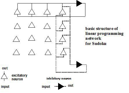
10.15 Parallel Search of Larger Memories. Searching many memory
modules can readily be carried out in parallel. Figure 12 shows the basic
multimodule circuit. There are many modules, which anatomically might
correspond to many hypercolumns. While this discussion will treat these
as separate and delineated (like barrel cortex in rats), the basic ideas de-
scribed here should be extendable to a cortex that is merely periodic and
less artificially modularized. Inputs come to corresponding cells in different
modules by branched axons from another brain area. Outputs from corre-
sponding cells in different modules are summed by pool cells. When the1144 J. Hopfield
ex
clue to the memory is substantial and the threshold parameter i thresh is prop-
erly set, a module queried with the clue will find the appropriate memory if
it is contained within the module, and will go to the all-off state otherwise,
as shown earlier. If the outputs from corresponding cells in all the modules
are summed by pool cells (see Figure 12), the output of the pool cells will
be due to the correct memory found by one of the modules, since all other
modules will have no output. This search is fast, requiring only the time
necessary for a single module to converge. The all-off state of each module
provides an automatic choice of the correct memory module to drive the
pool cells.
10.16 Parallel Search and Synchrony in the Case of Weak Memory
Clues. When the clue is rather small in size but still adequate for reliable
ex
retrieval, i thresh must be set so low that this simple procedure begins to fail
in a multimodule system. Another module that does not contain the correct
memory can settle into a junk state of activity, and the input to the pool
cells would consist of the correct memory from one module summed with
the junk state of another module. One conceptual possibility is that each
module explicitly evaluates whether it has found a true memory and sends
signals to the pool cells only if it has found a true memory. Any computation
that pop-out recognizes as a true memory could be used to gate the output
from a module. Such a method of operation would require neural circuitry
to explicitly gate each module. A more plausible possibility is to make use
of spike timing and synchrony, which could achieve the same result without
the need for additional circuitry or explicit gating.
A group of spiking neurons that have the same firing rate and are weakly
coupled often synchronize. This synchrony can be a basis for the many-are-
equal (MAE) operation, a recognition that a set of neurons is similarly driven
and not diverse in firing frequencies. MAE was usefully implemented for
speech processing (Hopfield & Brody, 2000; Brody & Hopfield, 2001). The
difference between the recollection of a correct memory and a junk state
is precisely that the correct memory has the firing rates of all neurons the
same. We therefore expect that if spiking neurons and appropriate synaptic
couplings are used instead of a rate model, a correct recall will result in
synchrony of the active model neurons, while a junk state would not result
in synchrony. When there is only a single module, synchrony can be used as
a means to detect correct versus junk states when the query information is
weak. Here, we discuss the extension of this idea to the problem of retrieval
of a memory from a multimodule system when the query information is
weak, so that modules may respond individually with the correct memory
or with a junk state.
The model description so far described has one neural unit for each point
in the category-property grid. Neurobiology would undoubtedly use more.
Suppose that we increase this number to 10 for each point, leaving all else the
same. These 10 will all get common input signals, will all send their axonsYou can also read