Electromagnetic, Thermal, Stress and Deformation Analysis of a Space-Based Satellite Dish Antenna
←
→
Page content transcription
If your browser does not render page correctly, please read the page content below
A      W H I T E              P A P E R            F R O M             A N S Y S ,                       I N C .

                  Electromagnetic, Thermal, Stress and
                  Deformation Analysis of a Space-Based
                         Satellite Dish Antenna
                                                                                                M.H. Vogel, ANSYS, Inc.

 T
ABSTRACT
THIS PAPER PRESENTS A MULTIPHYSICS ANALYSIS OF A SPACE-BASED COMMUNICATION SATELLITE DISH
antenna. Electromagnetic losses due to induced high-frequency surface currents lead to partial, asymmetric heating
of the structure, causing stress and deformation. A final electromagnetic analysis is performed on the resulting
deformed structure to determine the effect of the deformation on the antenna pattern and overall performance.

INTRODUCTION
Satellites in space often employ dish antennas to direct signals efficiently to a large but limited area of the earth’s
surface. For example, a satellite radio transmitter in geostationary orbit may, with an antenna beam width of a tenth of
a radian, cover most of the United States. The dish antenna may be illuminated by a small feed horn and connected
to the satellite by a metal waveguide or coaxial structure. Due to surface currents on the metals, a fraction of the
electromagnetic power is converted to heat. This causes a significant increase in temperature of the structure, since
there is no convection in the vacuum of space; heat can escape only through radiation, which is very weak at low
temperatures. Higher temperatures, as well as temperature differences between various parts, cause mechanical
stress and deformation. Simulation tools from ANSYS, specifically HFSS™ and ANSYS® Mechanical™ software — can
comprehensively analyze all these effects. Furthermore, the resulting deformed structure is brought back into the
electromagnetic simulation tool, HFSS, to determine how the deformations affect the antenna pattern.

ELECTROMAGNETIC ANALYSIS IN HFSS
The satellite with the dish antenna is depicted in Figure 1.

                                                                      Figure 1. Satellite with dish antenna

In most cases, the satellite transmits a digital signal. However, this digital signal may have a relatively modest
bandwidth (for example, a few MHz in the case of digital satellite radio) and is superimposed in encoded form on a

www.ansys.com                                                                                                              41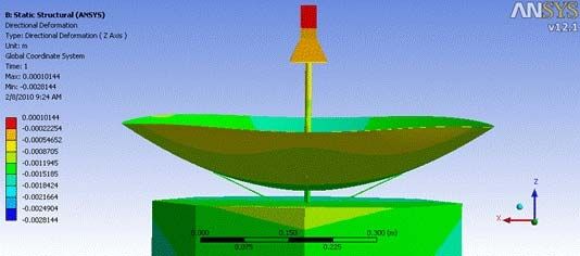
continuous-wave (CW) carrier signal with a much higher frequency, typically in the GHz range. This results in an
almost-CW signal with a bandwidth of the order of 0.1 percent. As a consequence, to determine the performance of
the microwave components and the antenna, it is enough to simulate the carrier wave.

For the design analyzed here, the signals from the satellite’s equipment travel through a coaxial metal structure,
through a coax-to-waveguide transformer to a feed horn that has its phase center in the focal point of the parabolic
dish. The dish is supported at the base of the coaxial guide and by four struts. The satellite is equipped with solar
panels for its energy supply.

The electromagnetic analysis is performed with High-Frequency Structure Simulator (HFSS) software from ANSYS.
HFSS employs the finite element method on an unstructured mesh that has small elements where needed and large
elements where possible [1], resulting in a simulation with optimum efficiency in memory and speed. A key
capability is adaptive meshing, in which the mesh is refined automatically in regions in which the field accuracy needs
to be improved.

The computational domain has an electrical size of 2,200 cubic wavelengths, and the final mesh had 263,000
elements. The simulation was done on a Windows® server using 20.7 GB of RAM and 119 minutes of total real time
from start to finish, including creation of the mesh and adaptive mesh refinement.

Key technologies employed, other than adaptive mesh refinement, were mixed-element orders, iterative matrix
solving and multi-core processing.

The term mixed-element orders refers to the orders of polynomials (the basis functions) that represent the electric
field in each mesh element. High orders are advantageous on a coarse mesh in regions in which fields are
smooth, while low orders in combination with a dense mesh are often the best choice in regions with large field
gradients, such as near metal edges. The mixed-element order technology, introduced for the first time with HFSS
version 12, intelligently applies the appropriate order in each element. As pointed out in [2], mixing orders can be
implemented best with so-called hierarchical elements, in which basis functions are constructed in families, such that
basis functions of a certain order are a subset of basis functions of the next higher order. This is because special care
needs to be given to the interfaces between elements in which different orders meet. Furthermore, orders are
adjusted where necessary as part of the mesh refinement process, so after several adaptations an accurate solution
is obtained efficiently with the optimum balance of element size and basis function order throughout the entire mesh.
All this is done automatically; the design engineer merely needs to specify an accuracy criterion.

The iterative solver [3] takes advantage of the aforementioned hierarchical basis functions by using the solution of a
lower-order representation of the finite element model as a preconditioner for the iterative solution of the full finite
element model. The preconditioner, being based on a lower order, is obtained in a short time with modest RAM usage.
Since the lower-order solution is a good starting point, already exhibiting key characteristics of the entire solution, the
iterative process subsequently obtains the full solution at very little additional cost.

Finally, multi-core processing runs processes in parallel wherever possible. Through so-called multithreading, the
computation of the preconditioner is spread out over multiple cores, achieving a speed-up of a factor of 2.5 to 3 when
using four cores. The iterative process after preconditioning is purely parallel in case of multiple excitations, running
the iterations for each excitation on a separate core.

www.ansys.com                                                                                                                 42
The antenna operates at 8.4 GHz. The dish has a diameter of 60 cm, which equals 17 wave lengths in this case. The
directivity is 31 dB with a 3-dB beam width of 4.5 degrees, and the first side lobes are 20 dB below the main
beam, as shown in Figure 2. For the application of a transmitter, for radio or mobile internet, the main antenna
design parameters are directivity and beam width, as these determine the reception in the area the radio
intends to cover. Side-lobe level is a parameter of interest when an antenna is used as a receiver. This
parameter determines to what extent signals from out-of-area transmitters may interfere. In general, 20 dB
down is considered a good side-lobe level.
                                                                The dish and its feed are made of light weight aluminium to
                                                                satisfy the always-present payload weight consideration
                                                                associated with space-based technologies. Due to the
                                                                metal’s finite conductivity, the surface currents induce
                                                                resistive losses in the metal, resulting in a fraction of the
                                                                power being converted into heat. Figure 3 shows the surface
                                                                loss density on a logarithmic scale on the surfaces of the
                                                                feed, feed horn and dish. The total surface loss is 25 W at an
                                                                input power is 500 W. The bulk of this loss takes place inside
                                                                the microwave components. The power density on the dish
Figure 2. Antenna pattern: peak directivity 31 dB, first side   is on average 1.8 kW/m2, of which only a few milliwatts per
lobes 20 dB below the main beam
                                                                m2 are lost while the rest is reflected.

THERMAL ANALYSIS
For the thermal simulation, the loss densities are mapped from the
HFSS analysis to ANSYS Mechanical and take the role of heat
load. The heat spreads through the entire structure at a rate
dependent on the thermal conductivities of the materials, and can
only escape in the form of thermal radiation to the surrounding
vacuum of outer space.

The heat loads are determined as follows:
For dielectric objects, such as Teflon® or plastic parts in the
structure or substrates in the electronics, the volumetric loss
density Q is given by                                                       Figure 3. Surface loss density
Q = 0.5    Re(E●Jconj)                         (1)
in which E is the complex electric field vector and J the volume current density. The latter is given by
J = σE                                         (2)
with σ the electric conductivity of the material. In case the electric conductivity is expressed as a loss tangent,
tan (δ), as it often is in material properties for frequencies in the GHz region, the relationship is
σ = ωε0εr tan(δ)                   (3)
in which ω is the angular frequency (2π times the frequency), and the product ε0εr is the total electric permittivity of
the material.

www.ansys.com                                                                                                                    43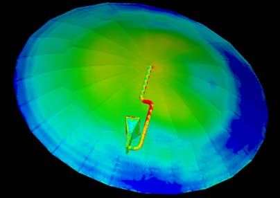
For metal objects, in principle (1) still applies. However, with a well-developed skin effect, currents flow in a layer of only micrometers thick along the surface, and they are more practically expressed as surface currents denoted by Js. The surface loss density Qs is given by Qs = 0.5 Re(Etan●Jsconj) (4) in which Etan is the tangential component of E along the metal surface and Js can be expressed by Js = Etan/Zs (5) In (5), Zs is the surface impedance, relating Etan and Htan through Etan = Zs (n×Htan) (6) For a good conductor, such as a metal with a well-developed skin effect, Zs is given by Zs = (1+j) √(ωμ0μr/2σ) (7) with the j the unit imaginary number √(-1), and the product μ0μr the total magnetic permeability of the metal. HFSS software solves for E, after which it computes the volume and surface loss densities automatically. ANSYS Mechanical technology links to the HFSS solution and maps the loss densities from the HFSS mesh to the ANSYS mesh. An advantage of this procedure is that the meshes need not be identical. An electromagnetic simulation often requires a denser mesh than a thermal or a structural simulation. Furthermore, the mapping between simulations gives the design engineer the freedom to include parts of the geometry in one simulation while excluding them in the other. For instance, the satellite body and the struts supporting the dish were not included in the electromagnetic simulation, because their interaction with the fields is negligible, but those structures were important in the thermal simulation. The steady-state thermal simulator solves the equation -● (k T) = Q (8) in which Q is the heat load imported from HFSS, k is the thermal conductivity tensor and T is the temperature. In case of a simple isotropic thermal conductivity, (8) simplifies to -k ΔT = Q (9) The minus sign expresses the fact that heat flows “downhill” from warm to cold. An important difference between thermal and electromagnetic simulations is that in the thermal case the unknown quantity, the temperature, is a real-valued scalar, while in the electromagnetic case, the unknown quantity, the electric field, is a complex-valued vector. As a consequence, if you have enough RAM for your electromagnetic simulation, you can expect that you will have more than enough for your thermal simulation. For this model, with 137,000 mesh elements, the simulation needed 795 MB RAM, 36 minutes CPU time and, thanks to the use of two cores, only 21 minutes real time. The finite element method applies a Q from HFSS software to every mesh element and subsequently solves for the distribution of temperature that fits this heat load, subject to boundary conditions. Without boundary conditions, no steady-state solution can be computed, as heat would continue to build up without limit. Common boundary condi- tions on outer surfaces are in general fixed temperatures, convection to account for air or fluid flow, and thermal radiation. In this case, since the satellite is in space, convection is zero and heat escapes only in the form of thermal radiation. The radiated power density on the surface is given by Prad = FB (T4-Tref4) (10) www.ansys.com 44
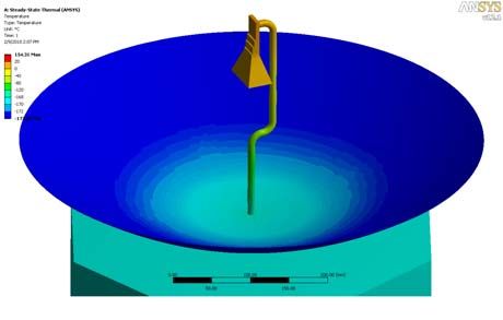
In this equation, F is the surface emissivity, with a value between 0 and 1, B is the Stefan–Boltzmann constant, with
a value of 5.669E-8 W/m2K4, and Tref is the background temperature, 3 K in this case. The resulting temperature
distribution is shown in Figure 4.
The highest temperatures are found inside the coaxial feed, in the coax-to-waveguide transformer and in the horn,
where the surface current densities are the highest. The lowest temperatures are found on the outer part of the dish,
since the thin dish has a relatively high thermal resistance.
Figure 4. Temperature distribution
MECHANICAL ANALYSIS
The resulting steady-state temperature distribution is used as the input for an analysis of stress and deformation. In
the simplest case, an increase in the temperature of an object leads to thermal expansion of that object, with a linear
relationship between the change in temperature and the change in length. In a general case, the increase in temper-
ature is not uniform, and/or the geometry consists of multiple materials with different expansion coefficients. This
leads to stress and deformation of the geometry. Both are of interest: The stresses need to be compared with the
strengths of connections between objects and the strengths of the materials themselves, while the deformation will
affect the operation of the antenna.
As for boundary conditions needed for a successful simulation, the user can apply kinematic constraints to constrain
rigid-body motion while allowing thermal expansion, or the user can fix the location of at least one face or assign
frictionless support to at least one face. For the case of a satellite in space, the location of the boundary condition is
arbitrary, and frictionless support was assigned to the top face of the horn. This makes it convenient to observe how
the reflector dish changes position and shape relative to the location of the horn.
The simulation required 431 MB RAM, 53 minutes CPU time and, thanks to the use of two cores, only 28 minutes real
time.
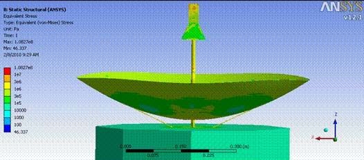
Figure 5 shows the thermal stresses in the structure. This result can be used to determine whether the struts are
strong enough. In this case, the struts experience a stress between 1 and 3 MPa, which is modest since aluminium
can withstand stresses of up to 300 MPa.
Of great interest is the thermal deformation of the dish and feed structure, since this affects the electromagnetic
performance and resulting radiation pattern. This is important, since deterioration in the pattern, if any, translates
directly into a deterioration of the reception of the signals on earth (in the case of satellite radio, a deterioration of
www.ansys.com 45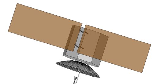
music reception by subscribers in a particular region). Figure 6 shows the deformation of the structure in the vertical
direction. Since this is a directional plot and the deformation takes place in the negative Z direction with the top of
the horn as a reference, all deformations are negative with that of the top of the horn closest to zero. The
deformation of the dish is between 1 mm and 2 mm for an input power of 500 W. Since the wave length is 36 mm,
this is a very small deformation. Still, one would like to know how much influence this has on the antenna pattern. To
this aim, the deformed geometry is exported to HFSS software.
Figure 5. Thermal stresses Figure 6. Deformation in the Z direction
ELECTROMAGNETIC ANALYSIS OF DEFORMED MODEL
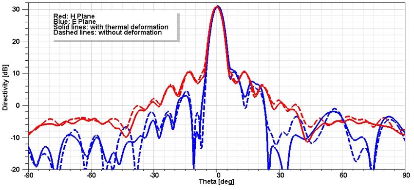
Once the deformed geometry has been imported into HFSS software, one can determine the antenna pattern. Figure
7 compares the antenna patterns of the deformed and original geometries. To eliminate any possible small
differences due to the use of different meshing methods, the original geometry was replaced by a geometry belong-
ing to a situation with negligible input power that had also been meshed and simulated in ANSYS®
Workbench™ Mechanical.
Figure 7. Comparison of antenna patterns of original and deformed structure
www.ansys.com 46Note that the impact of the deformation on the antenna pattern is very small. To some extent, this can be explained by the following observation: Due to thermal expansion, the distance between the horn and the dish increases. This would move the phase center of the horn away from the focal point of the dish and deteriorate the beam. At the same time, however, the dish widens a little, which moves the focal point up. So the focal point of the dish tends to follow the phase center of the horn. Even though the influence of the temperature turns out to be small in this case, it’s very important to perform analyses like this to be sure that the performance doesn’t deteriorate when the design operates at full power for a long time. CONCLUSION ANSYS HFSS technology was used to design a space-based satellite dish antenna and its feed structure consisting of a rigid coaxial transmission line, a coax-to-waveguide transition and a feed horn. The phase center of the horn is located in the focal point of the dish, and the horn–dish combination produces an antenna pattern with the desired coverage: the bulk of one continent on Earth. Having obtained an antenna design that meets the specifications, an investigation showed how the actual high-power operating conditions would affect performance. Electromagnetic losses in the microwave components generate heat, which results in a temperature gradient. This can be significant in the vacuum of space due to the absence of natural convection. The thermal gradients create a thermal deformation, which ultimately affects the electromagnetic performance of the device. In this case, the deformations were on the order of a couple of millimeters. The deformed geometry was used in a new electromagnetic simulation. The influence of the deformations was visible in the antenna pattern, but only at low levels and far from the main beam, so no structural modifications were needed. This example demonstrates the value of multiphysics simulation. The accuracy and connectivity between the various ANSYS simulation tools for electromagnetic, thermal and structural analyses enable the rapid evaluation of the satellite dish antenna operating under real-world multiphysics conditions. Combined together, HFSS and ANSYS Mechanical products form the foundation for comprehensive multiphysics simulation capable of solving industry’s most complex engineering challenges. REFERENCES [1] Shenton, D.N. and Cendes, Z.J. “Three-Dimensional Finite-Element Mesh Generation Using Delaunay Tesselation.” IEEE Trans. Magn., 1985, Vol. MAG-21, no. 6, pp. 2535–2538. [2] Silvester, P.P. and Pelosi, G. Finite Element for Wave Electromagnetics, IEEE Press, 1994; ISBN 0-7803-1040-3, Section “Hierarchal Elements”, p. 13. [3] Sun, D.-K., Lee, J.-F., Cendes, Z.J. “Construction of Nearly Orthogonal Nedelec Bases for Rapid Convergence with Multilevel Preconditioned Solvers.”Siam J. Sci. Comput., 2001. Vol. 23, No. 4, pp. 1053–1076. www.ansys.com 47
www.ansys.com
    About ANSYS, Inc.                                                                                 ANSYS, Inc.               Toll Free U.S.A./Canada:
    ANSYS Inc., founded in 1970, develops and globally markets engineering                            Southpointe               1.866.267.9724
                                                                                                      275 Technology Drive      Toll Free Mexico:
    simulation software and technologies widely used by engineers and design-
                                                                                                      Canonsburg, PA 15317      001.866.267.9724
    ers across a broad spectrum of industries. The Company focuses on the                             U.S.A.                    Europe:
    development of open and flexible solutions that enable users to analyze                            724.746.3304              44.870.010.4456
                                                                                                      ansysinfo@ansys.com       eu.sales@ansys.com
    designs directly on the desktop, providing a common platform for fast, efficient
    and cost-effective product development, from design concept to final-stage
    testing, validation and production. The Company and its global network of          ANSYS, ANSYS Workbench, AUTODYN, CFX, FLUENT, HFSS and any and
    channel partners provide sales, support and training for customers.                all ANSYS, Inc. brand, product, service and feature names, logos and
    Headquartered in Canonsburg, Pennsylvania, U.S.A., with more than 60               slogans are registered trademarks or trademarks of ANSYS, Inc. or its
    strategic sales locations throughout the world, ANSYS, Inc. and its subsidiaries   subsidiaries in the United States or other countries. All other brand, product,
                                                                                       service and feature names or trademarks are the property of their respective
    employ over 1,600 people and distribute ANSYS products through a network           owners.
    of channel partners in over 40 countries. Visit http://www.ansys.com for more
    information.                                                                       © 2010 ANSYS, Inc. All rights reserved.

www.ansys.com                                                                                                                                                            48
You can also read