ESTIMATING LOCAL AGRICULTURAL GROSS DOMESTIC PRODUCT (AGGDP) ACROSS THE WORLD
←
→
Page content transcription
If your browser does not render page correctly, please read the page content below

Earth Syst. Sci. Data, 15, 1357–1387, 2023
https://doi.org/10.5194/essd-15-1357-2023
© Author(s) 2023. This work is distributed under
the Creative Commons Attribution 4.0 License.

            Estimating local agricultural gross domestic product
                         (AgGDP) across the world
         Yating Ru1, , Brian Blankespoor2, , Ulrike Wood-Sichra3 , Timothy S. Thomas3 , Liangzhi You3 , and
                                                  Erwin Kalvelagen3
                       1 Department  of City and Regional Planning, Cornell University, Ithaca, NY, USA
                                2 Development  Data Group, World Bank, Washington, DC, USA
                         3 International Food Policy Research Institute (IFPRI), Washington DC, USA
                                         These authors contributed equally to this work.

                            Correspondence: Brian Blankespoor (bblankespoor@worldbank.org)

                                  Received: 3 October 2022 – Discussion started: 7 November 2022
                        Revised: 10 February 2023 – Accepted: 10 February 2023 – Published: 24 March 2023

       Abstract. Economic statistics are frequently produced at an administrative level such as the subnational di-
       vision. However, these measures may lack sufficient local variation for effective analysis of local economic
       development patterns and exposure to natural hazards. Agricultural gross domestic product (GDP) is a critical
       indicator for measurement of the primary sector, on which more than 2.5 billion people depend for their liveli-
       hoods, and it provides a key source of income for the entire household (FAO, 2021). Through a data-fusion
       method based on cross-entropy optimization, this paper disaggregates national and subnational administrative
       statistics of agricultural GDP into a global gridded dataset at approximately 10 × 10 km for the year 2010 using
       satellite-derived indicators of the components that make up agricultural GDP, i.e., crop, livestock, fishery, hunting
       and forestry production. To illustrate the use of the new dataset, the paper estimates the exposure of areas with at
       least one extreme drought during 2000 to 2009 to agricultural GDP, which amounts to around USD 432 billion
       of agricultural GDP circa 2010, with nearly 1.2 billion people living in those areas. The data are available on the
       World Bank Development Data Hub (https://doi.org/10.57966/0j71-8d56; IFPRI and World Bank, 2022).

1   Introduction                                                    lecting and reporting data across the world can be challeng-
                                                                    ing, especially in areas affected by fragility, conflict and vio-
                                                                    lence, which can result in incomplete or outdated geographic
According to the Food and Agriculture Organization (FAO)            coverage.
of the United Nations, at least 2.5 billion people depend on           Detailed agricultural data are critical to examining a wide
the agricultural sector for their livelihood, and it provides a     range of agricultural issues, including technology and land
key source of employment and income for poor and vulner-            use (e.g., Bella and Irwin, 2002; Luijten, 2003; Staal et al.,
able people (FAO, 2013, 2019, 2021). However, economic              2002; Samberg et al., 2016), exposure to natural hazards
statistics of the agricultural sector are frequently produced       (e.g., Murthy et al., 2015), evaluation of forest restoration op-
at a national or lower administrative level and may not ade-        portunities (Shyamsundar et al., 2022) as part of nature-based
quately capture local variation in production activities. Fur-      climate solutions (Griscom et al., 2017) and patterns and pro-
thermore, a geographic unit of interest, such as the natural        ductivity of economic development (e.g., Nelson, 2002; El-
area of a river basin, may not align with political administra-     horst and Strijker, 2003; Gollin et al., 2014; Reddy and Dutta,
tive boundaries, limiting the ability to conduct a comprehen-       2018). Carrão et al. (2016) examine the exposure of people
sive overlay analysis of the area. Lastly, local conditions can     and economic activity to drought using measures of physical
pose challenges to measurement across the world. Around 5           elements (e.g., cropland and livestock). Rentschler and Sal-
billion hectares of land is dedicated to agriculture, but col-

Published by Copernicus Publications.
1358                                                                       Y. Ru, B. Blankespoor, et al.: Local agricultural GDP

hab (2020) find that low- and middle-income countries have           2014). Uneven agricultural productivity across different re-
89 % of the global flood-exposed population, and poor peo-           gions or locations can lead to a non-uniform distribution of
ple account for almost 600 million who are directly exposed          labor within the sector, which has implications for the accu-
to the risk of intense flooding. Vesco et al. (2021) examine         racy and effectiveness of models based on rural per capita
linkages between climate variability and agricultural produc-        allocation. Other methods used land cover such as vegetation
tion as well as conflict. They find that climate variability con-    and built-up indices but did not however incorporate types
tributes to an increase in the spatial concentration of agricul-     of agriculture like cropland and livestock (Gunasekera et al.,
tural production within countries. Furthermore, in countries         2015; Goldblatt et al., 2019).
with a high share of agricultural employment in the national            Other methods to estimate GDP at a local level take advan-
workforce, they find that this combined effect increases the         tage of nighttime light datasets. Doll et al. (2006) and Elvidge
likelihood of conflict onset. To better target rural develop-        et al. (2009) found nighttime lights to provide a uniform, con-
ment strategies for economic growth and poverty reduction            sistent and independent estimate for economic activity, and
as well as conserve the natural resource base for long-term          several other studies (e.g., Chen and Nordhaus, 2011; Hen-
sustainable development, we need to accurately delineate the         derson et al., 2012; Ghosh et al., 2010; Bundervoet et al.,
spatial distribution of agricultural resources and production        2015; Wang et al., 2019; Eberenz et al., 2020; Wang and
activities (Wood et al., 1999).                                      Sun, 2021) utilized this striking correlation between lumi-
   One method to address the case where administrative               nosity and economic activities to estimate economic output
boundaries and geographic areas of interest are not aligned          on the ground. While night light is a good reflection of eco-
is to use the gridded (raster) data format. It provides an inter-    nomic activities in manufacturing and urban areas, nighttime
mediate and consistent unit for disaggregation and aggrega-          light data may not capture the agricultural activity as they
tion (e.g., UNISDR, 2011). Data-disaggregation methods can           require areas to emit light. Bundervoet et al. (2015) suggest
use detailed data to inform estimates of aggregated data from        that agricultural indicators rather than rural population could
large areas at the local level (e.g., see the review in Pratesi      improve the estimation of GDP given the importance of agri-
et al., 2015). Several spatial data products from global mod-        culture in many of the economies in their sample of Africa.
els are available to estimate population at a local level (see       Gibson et al. (2021) find that nighttime light data are a poor
the review in Leyk et al., 2019).                                    predictor of economic activity in low-population-density ru-
   Previous evidence-based risk analyses take advantage of           ral areas.
global data of hazards to estimate exposure of populations              In this paper, we present a high-resolution gridded agri-
and economic activity (e.g., Gunasekera et al., 2015, 2018;          cultural GDP (corresponding to the “agriculture, forestry,
Ward et al., 2020; Rentschler and Salhab, 2020). Gross do-           and fishing, value added” in World Development Indicators,
mestic product (GDP) is a critical economic indicator in the         henceforth AgGDP) dataset that is produced through a spa-
measurement and monitoring of an economy in a country                tial allocation model by distributing national and subnational
that is typically only available at national and occasionally        statistics to 5 arcmin grids based on satellite-derived infor-
subnational levels. Regional indicators play a key role in the       mation of constituents of AgGDP, including forestry, hunt-
necessary variation to forecast regional GDP (Lehmann and            ing and fishing, as well as cultivation of crops and livestock
Wohlrabe, 2015) and food security (Andree et al., 2020).             production.1 Our main contribution is to construct a global
Previous efforts to estimate local GDP use high-resolution           dataset of gridded AgGDP. This entails a massive effort of
spatial auxiliary information such as luminosity or popula-          data collection and integration. We extend and apply the
tion data to provide local variation. Methods by Nordhaus            cross-entropy framework developed in the Spatial Produc-
(2006), the World Bank and UNEP (2011), Kummu et al.                 tion Allocation Model (SPAM) for crops that pioneered the
(2018) and Murakami and Yamagata (2019) took advantage               use of cross-entropy optimization in spatial allocation (You
of gridded population data, which is the result of a model           and Wood, 2003; You et al., 2014, 2018; Yu et al., 2020). We
disaggregating the most detailed level of population data into       construct and integrate global datasets of the components of
grids. However, income is not evenly distributed among peo-          AgGDP as priors and then reconcile the values with the re-
ple or infrastructure (Berg et al., 2018). In fact, the divide be-   gional accounts statistics using cross-entropy optimization.
tween the rich and poor is even widening in our time (Dabla-         As an illustration of the novel dataset, we assess the exposure
Norris et al., 2015). The method used in the World Bank and          of economic activity to natural hazards with a focus on Ag-
UNEP (2011) stratifies the population by rural and urban,            GDP. Significant progress has been made to measure physi-
yet the definition of these geographic areas can vary based          cal assets such as built-up areas along with its importance in
on the selection of the population model (Leyk et al., 2019).        population models (Rubinyi et al., 2021) and estimate haz-
These measurements matter in application to stylized facts           ards in order to quantify the exposure to natural hazards (e.g.,
such as the strong negative correlation of the level of urban-
ization with the size of its agricultural sector (Roberts et al.,        1 Agriculture, forestry and fishing correspond to ISIC divisions
2017). Also, the strong assumption of uniform distribution           1–3 and include forestry, hunting and fishing as well as cultivation
of labor in agriculture is another key concern (Gollin et al.,       of crops and livestock production.

Earth Syst. Sci. Data, 15, 1357–1387, 2023                                            https://doi.org/10.5194/essd-15-1357-2023

Y. Ru, B. Blankespoor, et al.: Local agricultural GDP                                                                          1359

Gunasekera et al., 2015; UNDRR, 2019). However, the de-              not available globally. Therefore, we use the FAOSTAT na-
tailed spatial distribution of AgGDP is less known. So, we           tional producer prices and take the average of 2009–2011 in
apply these data to inform efforts quantifying the population        order to mitigate the potential impact of temporal variation.
and AgGDP at risk of drought and water scarcity, highlight-          However, due to missing data for certain countries, crops and
ing a linkage to a subset of agricultural activities as well as      years, this average may be based on a smaller time period
an association with population.                                      or the closest year available. As mentioned earlier, SPAM
   The rest of this paper is structured as follows. The next sec-    is a cross-entropy model, which calculates a plausible allo-
tion provides a detailed description of the methodology and          cation of crop areas and production to approximately 10 km
data. Then, we present the model results, uncertainty and val-       pixels, based on agricultural statistics at national and sub-
idation. Afterwards, we demonstrate one possible application         national levels, combined with gridded layers of cropland,
by analyzing AgGDP exposure to natural hazards. Finally,             irrigated areas, population density and potential crop areas
we provide concluding remarks.                                       and yields (Yu et al., 2020). SPAM’s output distinguishes be-
                                                                     tween 42 crops (33 individual crops, 9 aggregated crops) that
                                                                     together add up to practically all cultivated crops in a coun-
2     Methodology and data
                                                                     try with four parameters, i.e., production, yield, physical area
Following the composite structure of AgGDP, we disaggre-             and harvest area.
gate the national and subnational statistics into a global grid         For aggregated SPAM crops (such as other cereals, other
through a cross-entropy allocation model. Given the limited          pulses, vegetables or fruits), we computed their prices by tak-
availability of data and the global scope of the study, we           ing the weighted average of their components as follows:
made various efforts to adjust official statistics and create pri-                 6j pricej prodj
ors for different components based on the available data. Be-        PriceJagg =                     , ∀j ∈ Jagg,                (1)
                                                                                      6j prodj
low we discuss the construction of each component, AgGDP
statistics and the allocation model followed by the global nat-      where Jagg is the aggregated crop group, j is any crop that
ural hazard data. Given the spatial resolution and year of ref-      belongs to Jagg, PriceJagg is the price of the aggregated crop
erence of the input data for the crop value of production,           group, pricej is the price of crop j and prodj is the produc-
we estimate AgGDP for the year 2010 into 5 arcmin grids              tion of j .
(10 × 10 km) across the world.                                          For each grid, the value of crop production is thus

2.1     Construction of components                                   Cropvali = 6j prodi,j pricej , ∀j that grow in pixel i,     (2)

For each pixel, we construct an estimated value of production        where Cropvali is the value of total crop production in pixel
based on high-spatial-resolution information on the five com-        i, prodi,j is the production of crop j in pixel i and pricej is
ponents that serve as priors in the modeling process: crop,          the price of crop j . A map of the global gridded crop produc-
livestock, forestry, fishing and hunting. Given the lack of in-      tion value as a prior is shown in Fig. 1.
formation on the hunting component, we disaggregate the
forestry component into two parts: timber and non-timber             2.1.2   Livestock production
products of forestry. The non-timber products of forestry in-
clude an even distribution of hunting. The construction of the       Livestock accounts for an estimated 40 % of the global value
five components is described below in four subsections: crop,        of agriculture output and plays an important role in ensur-
livestock, forestry (timber and non-timber) and fishing.             ing the livelihood and food security of over one-sixth of the
                                                                     world’s population (FAO, 2018). However, it is still under
                                                                     rapid expansion as the global demand for animal-sourced
2.1.1    Crop value of production                                    products such as meat, milk, eggs and hides continues to
The prior for the crop component in the gridded AgGDP is             grow (Herrero and Thornton, 2013). While species and quan-
generated by multiplying the quantity of production from the         tities of livestock raised vary among regions and husbandry
global SPAM 2010 version 1 dataset2 (You et al., 2018) with          farmers, there are five primary species – cattle, sheep, goats,
producer prices at the country level from the Food and Agri-         pigs, and chicken – that prevail worldwide and provide es-
culture Organization Corporate Statistical Database (FAO-            sential products for human consumption.
STAT) (FAO, 2016) for each crop and then summed together.                We calculate the prior for the component of livestock pro-
As for the producer prices, ideally, we need subnational-level       duction in gridded AgGDP based on the distribution maps of
figures since prices for agricultural products can vary greatly      the above five primary species from the Gridded Livestock
within countries and their subdivisions, but such a dataset is       of the World (Robinson et al., 2014; Gilbert et al., 2018) and
                                                                     FAOSTAT’s value of production of livestock products (in-
   2 Available at https://www.mapSPAM.info (last access: 31 Jan-     cluding meat, milk, eggs, honey and wool) (FAO, 2020). Due
uary 2019).                                                          to data limitations, distribution maps for other animals such

https://doi.org/10.5194/essd-15-1357-2023                                            Earth Syst. Sci. Data, 15, 1357–1387, 2023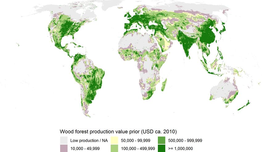
1360                                                                           Y. Ru, B. Blankespoor, et al.: Local agricultural GDP

Figure 1. The assembled crop production value used as a prior in the cross-entropy model (FAO, 2016; Yu et al., 2020).

as ducks, horses, camels and bees are not available. How-              Table 1. Conversion factors for different livestock types. Source:
ever, the FAOSTAT livestock production values include a                Eurostat (2018).
more comprehensive list of animals and their products. By
distributing FAOSTAT values to grids in proportion to the                             Livestock type    Conversion factor
five primary livestock species, we assume that other animals                          Cattle                            1
included in FAOSTAT have a similar spatial distribution to                            Pig                             0.3
the five primary livestock species. This assumption is gener-                         Goat                            0.1
ally valid but may not be accurate in special areas such as                           Sheep                           0.1
deserts, where camels are an important source of livestock                            Chicken                        0.01
products. To facilitate comparison, the animal-specific den-
sity numbers are converted to one animal type by using In-
ternational Livestock Units as conversion factors (Eurostat,           and X is a set including all pixels that fall within the bound-
2018) as shown in Table 1. The conversion factors reflect              ary of a nation.
biomass differences between different animals.3 Then the                  A map of global gridded livestock production value as a
densities of the animal-equivalent values are multiplied by            prior is shown in Fig. 2.
the total area of each 5 arcmin pixel to get the count of an-
imals per grid, which is used to calculate the share of ani-
mal counts and is then multiplied by the FAOSTAT value of              2.1.3    Forestry production and hunting
production to obtain the livestock production prior for each
pixel.                                                                 People have utilized forest resources for a long time through-
                                                                       out history for their livelihood and various other purposes
                   lsnumi                                              (Hossain et al., 2008). To date, over a billion people still rely
lsvali = lsvalx             , ∀i ∈ X,                          (3)
                  6X lsnumi                                            on forest resources for food security and income generation
                                                                       to some extent (FAO, 2018). In the world’s least-developed
where lsvali is the total value of livestock production in pixel       regions, 34 countries depend on fuel wood to provide more
i, lsvalx is the value of livestock production (meat, milk,            than 70 % of energy, of which 13 nations require 90 % of en-
eggs, honey and wool) that is reported at the national level,          ergy (FAO, 2018).
lsnumi is the total number of equivalent animals in pixel i               The contribution of forest production to AgGDP can be
    3 The uniform conversion factors may oversimplify local varia-     classified into two broad types: wood (logging) products and
tion in livestock patterns. Future work may consider using country-    non-wood forest products. Wood (logging) products are the
specific values of livestock products from FAOSTAT.                    most-exploited commodities in the forestry sector. The trees

Earth Syst. Sci. Data, 15, 1357–1387, 2023                                                https://doi.org/10.5194/essd-15-1357-2023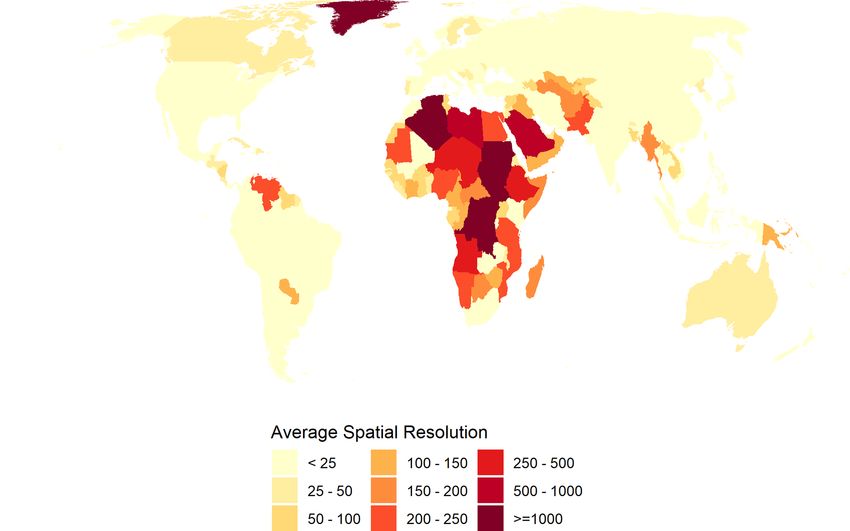
Y. Ru, B. Blankespoor, et al.: Local agricultural GDP                                                                                      1361

Figure 2. The assembled livestock production value used as a prior in the cross-entropy model. Sources: Robinson et al. (2014); Gilbert
et al. (2018); Eurostat (2018).

are harvested for fuel wood and industrial roundwood, which                 ing loss due to fire, with an assumption that the forests were
is processed into a variety of products, including lumber, ply-             mainly cut down for timber production. The Moderate Res-
wood, furniture and paper products. Non-wood forest prod-                   olution Imaging Spectroradiometer (MODIS) Land Cover
ucts are defined by the FAO.4 It is estimated that millions                 map (Friedl et al., 2010) for year 2011 is overlaid on top
of households around the world depend on non-wood for-                      of that for year 2010 to detect the area that has changed from
est products for their livelihood. Some 80 % of people in the               forest to non-forest.5 However, forest loss due to fire needs to
developing world use these products in their everyday lives                 be removed because it does not result in timber production in
(Sorrenti, 2016).                                                           most cases.6 Thus, fire information for year 2010 is obtained
   For a complete assessment of forest production priors, this              from the NASA Fire Information for Resource Management
study takes both wood and non-wood products into consider-                  System (FIRMS) (NASA, 2018), and areas that experienced
ation. The gridded non-wood forest products dataset used in                 forest fires are eliminated. After the identification of the for-
this study was jointly developed by Resources for the Future                est area change in each pixel, the value of wood production at
and the World Bank (Siikamäki et al., 2015) through an ap-                  the national level is taken from an FAO-led project (Lebedys
proach of meta-regression modeling, which integrates over                   and Li, 2014) and proportionally disaggregated to arrive at a
100 estimates at various locations from a literature review                 pixel-wise value of wood products as follows:
and multifold information on ecological and socioeconomic
factors. The value of non-wood forest products is resampled                 Woodvali = (forestvalx − nonwoodvalx )
to the 5 arcmin grid cell size and converted to 2010 USD for
                                                                                        forestlossi
consistency with other AgGDP components. As part of non-                                              , ∀i ∈ X,                               (4)
timber products, we include hunting with an even distribution                          6X forestlossi
across units and time given the lack of information.
   The value of wood products prior per pixel is calculated                    5 The measurement is limited to detection of land cover change
based on forest loss from year 2010 to year 2011 exclud-                    from satellites and might not fully account for selective harvesting
                                                                            or forest degradation. The area of forest is considered homogeneous
    4 These products are “goods of biological origin other than             and of equal production value. Also, it could result in upward bias
wood derived from forests, other wooded land and trees outside              when trees are cut down for plantation replanting and not used in
forests”, including foods (nuts, fruits, mushrooms, etc.), food ad-         further processing of timber production.
ditives (herbs, spices, sweeteners, etc.), fibers (for construction, fur-       6 Still, sometimes wood harvests may occur after forest fires, and
niture, clothing, etc.) and plant and animal products with chemical,        therefore the elimination could underestimate the area harvested for
medical, cosmetic or cultural value.                                        wood products.

https://doi.org/10.5194/essd-15-1357-2023                                                    Earth Syst. Sci. Data, 15, 1357–1387, 2023
1362                                                                       Y. Ru, B. Blankespoor, et al.: Local agricultural GDP

where Woodvali is the value of wood products in pixel i,             where fishvali is the value of fishery production in pixel i,
forestvalx is the value of forest products reported at the na-       freshvalx is the value of fresh fish production at the national
tional level, nonwoodvalx is the value of non-wood products          level which is aggregated from FISHSTAT, waterbodyi is the
at the national level which is derived from Siikamäki et al.         area of water bodies in pixel i and X is a set including all
(2015), forestlossi is the area of forest loss excluding loss        pixels i that fall within the boundary of a nation x.
to fire in pixel i and X is a set including all pixels that fall        The value of marine fishery production is determined by its
within the boundary of a nation.                                     proximity to fish landing ports and a composite indicator that
   In our analysis of the forestry sector GDP, we have utilized      equally weighs the number of vessel visits and the total hold-
the estimates provided by Lebedys and Li (2014) as the best          ing capacity of the fishing vessels. We use the port database
available source. However, it should be noted that these esti-       from the World Port Index (National Geospatial-Intelligence
mates primarily capture activities within the formal forestry        Agency, 2019) and the number of port visits with a vessel
sector and do not take into account the value added generated        hold of fishing vessels from Hosch et al. (2019) to create a
by informal activities such as wood fuel production and non-         composite variable as the prior based on the sum (for each
wood forest products. To account for non-timber forest prod-         port) of the number of visits (each event in the database) and
ucts, we have utilized the estimates provided by Siikamäki           the total vessel hold at the port. The geographic coverage
et al. (2015). Despite these efforts, it is acknowledged that        of the ports is calculated for each port using the minimum
the current analysis may still underestimate the forestry sec-       port distance provided in Hosch et al. (2019). Any distances
tor GDP due to the lack of reliable data on fuel wood pro-           greater than 150 km were considered to be 150 km in this
duction, which could account for half of global wood har-            analysis. The value of marine fishing production in each grid
vests (Ghazoul and Evans, 2004). This is a common issue as           is calculated as follows:
fuel wood values are often not properly captured in official
statistics, as they are often collected for subsistence or sold in                               portindexi
                                                                     marinevali = marinevalx                  , ∀i ∈ X,             (6)
remote rural areas in many countries (Lebedys and Li, 2014).                                    6X portindexi
In future research, we intend to make efforts to acquire more
reliable data on fuel wood production to improve the accu-           where marinevali is the value of fishery production in pixel
racy of our estimates of the forestry sector GDP.                    i, portindexi is an equally weighted composite index of the
   A map of global gridded wood forest production value as           number of visits and the total vessel hold in pixel i and X is
a prior is shown in Fig. 3.                                          a set including all pixels i that fall within the boundary of a
                                                                     nation x.
                                                                        A map of global gridded fishery production value as a prior
2.1.4   Fishery production                                           is shown in Fig. 4.

Fish makes up approximately 17 % of animal-sourced pro-
tein in the human diet worldwide (Mathiesen, 2018). The              2.2   AgGDP statistics and linked grids
fishery industry supports the livelihood of 12 % of the
world’s population by creating 200 million jobs along its            Substantial efforts have been made to collect and organize
value chain. In the global trade system, USD 80 billion worth        national and subnational statistics from a variety of sources,
of fish is exported from developing countries, and it plays          including national ministries and reports. However, not ev-
a crucial role in promoting local economic development               ery country publishes its AgGDP figures at the subnational
(Kelleher et al., 2009).                                             (regional) level, and there exist different methods of region-
   We estimate both freshwater inland fishery and marine             alization, including top-down, bottom-up and mixed meth-
production values using the FISHSTAT (FAO, 2009) data                ods (Eurostat, 2013).7 Our database has 68 countries that
with a classification based on the fish production categories.       have subnational AgGDP data, expressed in varying domes-
The inland fishery production value is the result of disag-          tic currencies and for different years. The typical adminis-
gregating corresponding country-level statistics in proportion       trative level is at the state or provincial level. Table B7 lists
to areas of inland water bodies in the 5 arcmin pixel. This          these countries and descriptive statistics, including the tem-
is a simplified assumption and may cause overestimation in
places where there are inland water bodies but not many fish-           7 Regional Gross Domestic Product (RGDP) can be estimated
ery activities going on. The distribution of inland water bod-
                                                                     following the production, income or expenditure approaches. How-
ies is obtained from the ESA-CCI (Lamarche et al., 2017).            ever, RGDP is not typically compiled using the expenditure ap-
Thus, the value of inland fishing production in each grid is         proach due to the scarcity of data such as interregional purchases
calculated as follows:                                               and sales or regional exports/imports. In the production and income
                                                                     approaches, the estimate of market activities is typically from the
                        waterbodyi                                   production approach, whereas the estimate of non-market industries
fishvali = freshvalx                 , ∀i ∈ X,                (5)    is from the income approach.
                       6X waterbodyi

Earth Syst. Sci. Data, 15, 1357–1387, 2023                                            https://doi.org/10.5194/essd-15-1357-2023
Y. Ru, B. Blankespoor, et al.: Local agricultural GDP                                                                                  1363

Figure 3. The assembled wood forest production value used as a prior in the cross-entropy model (Friedl et al., 2010; Siikamäki et al., 2015;
NASA, 2018).

Figure 4. The assembled fishery production value used as a prior in the cross-entropy model (FAO, 2009; Lamarche et al., 2017; Hosch
et al., 2019; National Geospatial-Intelligence Agency, 2019).

poral coverage and the number of subnational regions at an               sistent and comparable for countries across the world, shares
administrative geographic level, including the NUTS level.8              from subnational statistics are calculated and then applied to
  To overcome discrepancies in temporal coverage and cur-                a national total to derive a calibrated number at the subna-
rency terms (constant and current) and to keep the data con-             tional level. The national totals are obtained from the pub-
                                                                         licly available World Development Indicators (WDIs) (World
    8 The European Union developed a standard for administrative
                                                                         Bank, 2019) and averaged over 3 years around 2010. For a
levels: the Classification of Territorial Units for Statistics (NUTS,    few countries that do not report their national AgGDP in the
for the French nomenclature d’unités territoriales statistiques).

https://doi.org/10.5194/essd-15-1357-2023                                                Earth Syst. Sci. Data, 15, 1357–1387, 2023
1364 Y. Ru, B. Blankespoor, et al.: Local agricultural GDP
WDI database, sums of all AgGDP components are used as The first step is to transform all real-value parameters into
proxies. corresponding probabilities. Let Si be the share of the total
The World Bank compiles these national accounts data AgGDP allocated to pixel i within a country x. AgGDPi,x is
following the International Standard Industrial Classifica- the AgGDP allocated to pixel i in country x, and X is a set
tion (ISIC) divisions 1–3 that include agriculture, forestry including all pixels that fall within the boundary of a nation.
and fishing. Given the challenges of compiling national ac- Therefore,
counts data across the world, limitations include the exclu-
AgGDPi,x
sion of unreported economic activity in the informal or sec- Si = , ∀i ∈ X. (7)
ondary economy. In particular, agricultural output in devel- 6X AgGDPi,x
oping countries may not be reported due to issues such as
Let PreAgGDPi be the pre-prior allocation of the AgGDP
natural losses or self-consumption and may not be exchanged
share from our best estimate. The first approximation can be
for money. Despite best efforts, agricultural production may
done by summing all five calculated pixel-level components
be estimated indirectly, leading to approximations that are
of AgGDP:
different than the true values.9
The calibrated statistics are then linked to grids through a PreAgGDPi = Cropi + Livestocki + Forestryi
shapefile of the Global Administrative Unit Layers (GAUL)
+ Fishingi + Huntingi , (8)
that maintains global geographic layers with a consistent and
comprehensively unified coding system (FAO, 2015). Then, where we assume hunting occurs in areas with equal proba-
we overlay the GAUL administrative boundaries on the grid bility.
network to assign the corresponding codes of the administra- Theoretically, the sum of these components should be
tive units to each grid.10 For areas where subnational Ag- close to the official values obtained from the World Devel-
GDPs have different administrative areas than GAUL, the opment Indicators. However, it should be noted that due to
GAUL areas are merged or split to match the subnational limitations in the available data, we have some components
AgGDP areas. in output values (crop, livestock and fishery), whereas others
in value added are added (forestry and hunting). This may re-
sult in discrepancies and inconsistencies. Overall, we make
2.3 Spatial allocation model sure that the official AgGDP values are guaranteed to be no
After constructing all the components, we define a spatial al- less than the sum of all five components of AgGDP.
location model in a cross-entropy framework following You
AgGDPx = 6i∈x PreAgGDPi (9)
et al. (2014) to allocate administrative statistics to 5 arcmin
pixels.11 National and subnational AgGDP values are used as Then we rescale the prior AgGDP to be consistent with the
a constraint, while the distribution of crop, livestock, fishery official AgGDP value:
and forestry production (hunting is included in non-timber
products of forestry) is used to create priors for estimating PreAgGDPi AgGDPx
PriorAgGDPi = . (10)
pixel-level AgGDP. In actuality, the priors that we have con- 6i PreAgGDPx
structed do not encompass all elements of AgGDP, and the
Then we calculate the prior for Si as a probability by nor-
national and subnational AgGDP statistics include a broader
malizing PriorAgGDP:
range of production values. However, the priors account for
most variation between pixels, and thus their shares can serve PriorAgGDPi,x
as appropriate proxies in the AgGDP disaggregation model. PreAlloci = . (11)
6i∈X PriorAgGDPi
Lastly, measurement units are unified using deflators and ex-
change rates.12 Finally, we formulate a cross-entropy model in the follow-
ing mathematical optimization framework:
9 See https://data.worldbank.org/indicator/NV.AGR.TOTL.ZS
MIN CE(Si ) = 6i Si log(Si ) − 6i Si log(PreAlloci ), (12)
(last access: 31 January 2019) for more details on metadata and
limitations.
10 For presentation purposes, a country may refer to a sovereign subject to the following three conditions:
country or other political area such as a dependency or disputed 6i Si = 1, (13)
area.
11 A comprehensive presentation of the cross-entropy method is 6i∈k (6AgGDP)Si = SubAgGDPk ∀k, (14)
in Rubinstein and Kroese (2004). 0 ≤ Si ≤ 1∀i, (15)
12 The currency varies by source. Crops are in local currency.
Livestock are in International USD 2004–2006. Fish are in USD where i: i = 1, 2, 3, . . . are pixel identifiers within the al-
2009. Non-timber forest products are in USD 2012, and timber (for- location unit (e.g., Brazil) and k: k = 1, 2, 3, . . . are iden-
est) products are in USD 2011. tifiers for subnational geopolitical units (e.g., a state) where
Earth Syst. Sci. Data, 15, 1357–1387, 2023 https://doi.org/10.5194/essd-15-1357-2023Y. Ru, B. Blankespoor, et al.: Local agricultural GDP 1365
AgGDP values (SubAgGDPk ) are available. The objective We examine the correlation of the AgGDP dataset with
function is defined as the cross-entropy of AgGDP shares and two commonly used global datasets to proxy economic ac-
their priors. The first constraint (Eq. 13) is the pycnophylac- tivity: nighttime lights and population. Nighttime light data
tic or volume-preserving constraint (e.g., Tobler, 1979) that are commonly used in the estimation of local human de-
ensures the sum of all allocated AgGDP values is equal to velopment and economic activity (e.g., Ghosh et al., 2010;
the total AgGDP of the country. The next Eq. (14) sets the Henderson et al., 2012; Bundervoet et al., 2015; Kummu
sum of all allocated AgGDP values within those subnational et al., 2018; Bruederle and Hodler, 2018). We use the sum
units with available data to be equal to the corresponding of the radiance-calibrated data for 2010 from the F16 satel-
subnational AgGDP values. The last Eq. (15) is a natural lite to quantify the correlation between AgGDP and night-
constraint for the share of AgGDP to be between 0 and 1, time lights by geographic regions of the world defined by the
which is also the probability in the cross-entropy model. The World Bank.15 We use rural population derived from Cen-
modeling framework is flexible in that more constraints can ter for International Earth Science Information Network –
be added if more data are available and/or more reasonable CIESIN – Columbia University (2017) following methods in
assumptions about how AgGDP should be spatially disag- Thomas et al. (2019). We use country-level data from the
gregated are discovered.13 Last but not least, we multiply the World Bank World Development Indicators (World Bank,
total regional AgGDP by the probability in the cross-entropy 2019). We find that the correlation of AgGDP with night
model to derive the final pixel-level AgGDP: light varies across world regions, with sub-Saharan Africa
and the Other region showing lower correlation values (Ta-
AgGDPi = 6i AgGDPx Si . (16) ble 2). Most World Bank regions have similar patterns of cor-
relation with nighttime lights across the measures of AgGDP
and population. Likewise, World Bank income groups show
3 Results, uncertainty and validation
similar patterns across the measures, with the lower-middle
3.1 Results and upper-middle income groups having higher correlations
than the low- and high-income groups. However, notable dif-
Figure 5 illustrates the result of the cross-entropy model in a ferences in the correlations exist between geographic levels.
global map of the gridded AgGDP. The global gridded Ag- The mean correlation of AgGDP with nighttime lights (NTL)
GDP for the year 2010 in 2010 USD is in gridded (raster) and population (pop) derived from administrative level-2
format at a resolution of 5 arcmin, which approximates to data is lower than the national level, which presents evidence
10 km.14 The spatial extent and quantity distribution of Ag- of new information from the AgGDP dataset.
GDP over the world are in agreement with general knowl- Furthermore, limitations exist with these commonly used
edge of agricultural technology adoption and suitability, with datasets for applications of AgGDP. For nighttime lights, Li
well-known agricultural nations such as India, China and the et al. (2020) provide a cautionary note about rural applica-
United States standing out as regions with relatively high Ag- tions where the presence of agricultural activities typically
GDP compared with many other areas of the world. A num- takes place. A population model assumes proportional ac-
ber of European countries also exhibit high AgGDP values, tivity to population by strata (e.g., rural), which does not
which is likely due to the benefit of adopting mechanized account for the type of rural of agricultural activity, and
farming and technological facilitation, considering that the the model requires a standard definition of rural, which can
shares of agricultural land and agrarian population are rela- pose challenges in global applications (e.g., stylized facts
tively low in these well-developed places. Countries in sub- in the urban and development economics literature Roberts
Saharan Africa remain low in agricultural production, as in- et al., 2017). Notably, the rural population dataset also has
dicated by low-value pixels sparsely spreading over the con- variation in the geographic level of the input information,
tinent. Within the continent, agricultural production activi- which informs the estimates of population models and cur-
ties primarily take place in geographic areas with suitability rency across the world, especially when dependent on the
and access to markets (e.g., land cultivation; see Berg et al., frequency of production and the availability of a population
2018). census. Also, the AgGDP dataset may attenuate modeling
concerns of endogeneity when using AgGDP along with pop-
13 For instance, market access may play a role in determining the
ulation or nighttime lights.
spatial distribution or spatial structure of AgGDP and can be in-
cluded as a constraint in the model. However, we provide a parsi-
monious model without market access.
14 The coordinate system is the standard WGS84 and is saved in
GeoTIFF format. For presentation in the paper, the coordinate sys-
tem of the maps is Eckert IV and is transformed from the geographic
coordinates in the R software. The data are publicly and freely avail- 15 Specifically, we use the version 4 product from the F16 satel-
able through the World Bank Development Data Hub website at lite (20100111 to 20101209) available at https://ngdc.noaa.gov/eog/
https://doi.org/10.57966/0j71-8d56 (IFPRI and World Bank, 2022). dmsp/download_radcal.html (last access: 15 June 2016).
https://doi.org/10.5194/essd-15-1357-2023 Earth Syst. Sci. Data, 15, 1357–1387, 20231366 Y. Ru, B. Blankespoor, et al.: Local agricultural GDP
Figure 5. Global gridded AgGDP circa 2010 from the cross-entropy model in 2010 USD.
Table 2. Spearman correlation of AgGDP with nighttime lights at the Admin 0 level (1) and Admin 2 level (2) as well as the rural populations
at the Admin 0 level (3) and Admin 2 level (4), grouped by World Bank region where AFR is sub-Saharan Africa, EAP is East Asia and the
Pacific, ECA is eastern Europe and central Asia, LAC is Latin America, MENA is the Middle East and North Africa, SOA is South Asia,
and Other is the category for the remaining countries (NOAA, 2011; World Bank, 2019).
AgGDP correlations by (1) (2) (3) (4)
World Bank regions NTL (adm 0) NTL (adm 2) POP (adm 0) POP (adm 2)
AFR 0.682 0.314 0.934 0.673
EAP 0.956 0.493 0.979 0.739
ECA 0.818 0.546 0.914 0.611
LAC 0.949 0.605 0.947 0.720
MENA 0.798 0.556 0.953 0.638
Other 0.896 0.669 0.909 0.697
SOA 0.929 0.547 0.929 0.716
3.2 Fitness for use and uncertainty may still be suitable for use, as it is already standardized in
grid cells, which may facilitate integration with other data.
We provide descriptive statistics of the data and modeling As the spatial refinement of ancillary data advances along
from a fitness-for-use perspective (e.g., Leyk et al., 2019). with greater currency, coverage and representativeness, we
The data are most appropriate for applications at global, con- expect validation possibilities to increase and inform a bet-
tinental and regional scales (You and Wood, 2006). However, ter understanding of the uncertainty and the associated fit-
decisions regarding the use of the data at smaller spatial ex- ness for use. Also, we intend to improve spatial and temporal
tents should be made with caution and with consideration of coverage when this is feasible.
the underlying assumptions and characteristics of the area in The process of disaggregating the data from the source
question. Users should take into account factors such as area level to the target level does impose spatial relationships and
of the grid cell of AgGDP, the number of subdivisions of Ag- is prone to error (Li et al., 2007) and the modifiable areal
GDP from the political area (e.g., country) and assumptions unit problem (MAUP) (Openshaw, 1981). In previous work,
in the priors (e.g., see shares of priors in Table B8). When our team conducted sensitivity analyses and examined the
input data contain multiple observations, the AgGDP dataset consequences of methodological-data choices involved in a
Earth Syst. Sci. Data, 15, 1357–1387, 2023 https://doi.org/10.5194/essd-15-1357-2023Y. Ru, B. Blankespoor, et al.: Local agricultural GDP 1367
cross-entropy model to disaggregate crop production statis- ded Livestock of the World (GLW) 2.0, we summarize the
tics (Joglekar et al., 2019). These analyses included eight sce- average spatial resolution (ASR) of the input regional data,
narios that varied in allocation methods, data groupings, in- which is the square root of the land area divided by the num-
put variables and different levels of statistics. The analysis ber of administrative units (see Fig. 6). We find that on av-
indicated that allocation results are most dependent on the erage the ASR value increases from high- to low-income
degree of disaggregation and the quality of the underlying groups based on World Bank 2010 classifications. Following
national and subnational production statistics. Therefore, we Yu et al. (2020), we suggest that users can view the ASR map
provide more discussion in Sect. 3.2.1 (Regional accounts). as an indicator of uncertainty level since the model is proven
Additionally, the results are moderately sensitive to alloca- most dependent on the ASR of statistics. A larger ASR rep-
tion methods. We previously compared three models for the resents more sparsity of input statistics and more uncertainty
case of Brazil (Thomas et al., 2019) and found that cross- of the gridded results.
entropy is the most appropriate method for the global study,
with relatively high accuracy and flexible data requirements 3.2.2 Components
when compared with either the spatial regression or rural
population methods. Interested readers may find more details Another source of uncertainty is the indirect temporal inaccu-
in the Brazil paper. Lastly, the results are somewhat sensitive racy propagated from the input datasets of the components,
to the groupings and formats of input components that serve which are modeled. We discuss all five components of Ag-
as priors, which we discuss in Sect. 3.2.2 (Components). GDP: crop, livestock, forest, fish and hunting. The SPAM
model (You et al., 2014) is a result of several gridded mod-
eled datasets, including rural population density from the
3.2.1 Regional accounts
Global Rural-Urban Mapping Project (GRUMP) Alpha ver-
The measurement of GDP is challenging (Angrist et al., sion (Balk et al., 2006). Likewise, the Gridded Livestock
2021), especially agricultural production (Carletto et al., of the World v2.0 includes rural population density in 2006
2015). The level of uncertainty associated with these results (GRUMP) along with other predictors such as precipitation
includes the thematic, spatial and temporal accuracies. We (Hijmans et al., 2005) and a modeled travel time to places
collected regional accounts by sector from various sources with 50 000 inhabitants circa 2000 (Nelson, 2008). Anderson
into a global database. The data are not balanced over time et al. (2015) find variation in their examination of global data
or at the geographic level. The variation in the reference year products of cropping system models. For livestock, we trans-
of the regional accounts data influences the temporal balance form the five major livestock types into international values
of the database. This mismatch can influence the regional dis- from livestock products (i.e., meat, milk, eggs, honey and
tribution of the AgGDP that may be different than the target wool). The forest (non-wood products, wood products) com-
reference year of 2010. Given climate16 and specifically rain- ponents rely on a remote-sensing model to estimate forest
fall are important inputs to crop and livestock production and loss. With regards to the non-timber values, limitations from
may contribute to variation across years (Stanimirova et al., the sources present two challenges. The estimates use simple
2019; Zhang et al., 2020), we attempt to reduce this source of averages from the literature that accordingly assume a prop-
error by averaging over multiple years when data are avail- erty of uniformity in the value of a hectare of forest to be
able, which is a similar approach to You et al. (2014). How- similar across the world, and the sample of forests with the
ever, this does not eliminate this mismatch. The availability literature drawn for the study is representative of the world
of data varies when grouped by World Bank income (low or (Siikamäki et al., 2015). The fishing model relies on the prox-
lower-middle, upper-middle and high income). The average imity and association with ports or water bodies.18 Finally,
absolute temporal difference (ATD) defined as the mean dif- since we do not incorporate any information on hunting, the
ference in years between the reference regional accounts and result is an even distribution across units and time.
the target year (2010) is higher in the low and lower-middle Another source of uncertainty is the geographic distribu-
income groups. Likewise, the mean deviation of the share of tion of the components. Ideally, we would use subnational
AgGDP by country over the year(s) is larger in the low- or prices; however, this was not feasible. So, the results do not
lower-middle income groups compared to the high-income reflect this occurrence, and there is a potential misrepresenta-
one. tion of administrative units with high variation of prices due
The global regional accounts database includes national to the heterogeneity of distinct urban and rural areas.
and subnational units at various administrative levels.17 Fol-
lowing Robinson et al. (2014) in their assessment of Grid- 3.3 Validation
16 For a discussion on climate yield factors, see Block et al.
A true validation of the predictive accuracy of this model in-
(2008). volves data collection and construction of agricultural gross
17 This also includes cases where administrative units at the same
level are merged to match the geography of the regional accounts 18 The freshwater case does not account for any variation, whereas
data. the marine port locations incorporate variation in vessel holds.
https://doi.org/10.5194/essd-15-1357-2023 Earth Syst. Sci. Data, 15, 1357–1387, 20231368 Y. Ru, B. Blankespoor, et al.: Local agricultural GDP Figure 6. The average spatial resolution of the regional accounts data by country (World Bank, 2019). See also the various sources in the Appendix. regional products in different pixels and testing those inde- gression model was slightly better than the cross-entropy pendent observations against the predicted values. The re- model, but it can hardly generalize to the global work since gional production data are, however, generally constructed at for many countries we only have one number at the national the administrative level rather than the pixels, so validation level and do not have enough degrees of freedom for the would have to be done on an aggregation of model predic- regression model. The naïve rural population model had a tions. Few countries provide the required data to assess the correlation value of 0.81 between the predictions and actual prediction accuracy to examine the internal validation of the values at the municipio level, and MAD and RMSE were disaggregation efficiency, and the data collection would be 28 744 and 25 397, respectively. The cross-entropy model extremely costly and time-consuming. An evaluation of pre- was proven to have relatively high accuracy compared to diction accuracy requires input data at a local level, which is the naïve model and better flexibility to accommodate data not available for all countries. scarcity in certain countries and thus was chosen as the model Multiple geographic levels of AgGDP exist for the case of for the global AgGDP dataset. Brazil, where we conducted a pilot study and examined the At the global scale, since we do not have AgGDP statis- validity of various methods to disaggregate AgGDP spatially, tics at lower administrative levels consistently, we are not including cross-entropy, a rural-population-based model and able to validate estimated results by aggregating to differ- spatial regression (see Thomas et al., 2019). Administrative ent geographic levels like the Brazil case. In addition, due to divisions of Brazil consist of 558 microregions, which are the volume-preserving pycnophylactic property of the cross- further divided into 5564 municipios. We had AgGDP data entropy model that utilizes all available data from mixed lev- at both the microregion and municipio levels. In order to els and ensures that the aggregated values conform to all the test the methods, we only used statistics for the 558 mi- original values, we do not have extra data for validation. All croregions and allocated them to gridded pixels. Then we available data have been internalized by the model to im- aggregated estimated results at the pixel level to 5564 mu- prove estimation results and thus cannot serve as external nicipios and compared them with ground-truth data. Results validation. Nevertheless, we compare the results from the showed that the correlation between the predictions and ac- global cross-entropy model to that from a rural population- tual values at the municipio level was 0.91 for the cross- based model at the grid level and examined their correlation, entropy model. Mean absolute deviation (MAD) and root which is a similar assessment to You et al. (2014) (as men- mean square error (RMSE) were 8249 and 18 347, respec- tioned, a spatial regression model at the global scale is not tively, while the average of the municipio-level true values feasible due to insufficient degrees of freedom). We construct was 28 739 (BRL 1.000). The performance of the spatial re- a proportional allocation model using rural population count Earth Syst. Sci. Data, 15, 1357–1387, 2023 https://doi.org/10.5194/essd-15-1357-2023
Y. Ru, B. Blankespoor, et al.: Local agricultural GDP                                                                        1369

following the method in Thomas et al. (2019) for the case           mation Network (CIESIN), Columbia University (2018).19
of Brazil. We use the 2010 Gridded Population of the World          For a drought index, we calculate the Standardized Precipita-
version 4 from Center for International Earth Science Infor-        tion Evapotranspiration Index (SPEI) (Vicente-Serrano et al.,
mation Network – CIESIN – Columbia University (2017)                2010), which measures the difference between observed pre-
adjusted to the United Nation’s World Population Prospects          cipitation and estimated potential evapotranspiration with a
followed by including the rural area defined by the Global          3-month interval using the base climatology of 1980 to 2019,
Human Settlement grid for 2015, i.e., “Rural cluster”, “Low         which is implemented in R (Beguería and Vicente-Serrano,
Density Rural grid cell” or “Very low density rural grid cell”      2017) using climate data from Harris et al. (2020). Extra-dry
(Pesaresi and Freire, 2019). We disaggregate national or sub-       years are defined as the number of years that are less than
national AgGDP statistics to grids in proportion to their ru-       or equal to −2.0 during the period from 2000 to 2009. Fig-
ral population, with each rural individual receiving an equal       ure A1 shows the results of the SPEI. The Water Crowding
portion of the AgGDP. Figure 7 shows results of the rural per       Index (WCI) is a measure of water scarcity considering the
capita model and the cross-entropy model together. We can           local population as the annual water availability per capita
test the similarity of the two global maps. Following Levine        (Falkenmark, 1986, 2013). Veldkamp et al. (2015) model the
et al. (2009), we assume a normal distribution over the 2 mil-      global WCI with return periods. We take the mean of any pix-
lion land pixels and perform a pairwise Student’s t test to test    els of the ensemble WCI with a 10-year return period within
the null hypothesis that both maps were identical. This test        an AgGDP pixel. Following the literature (e.g., Arnell, 2003;
allows us to examine whether the mean difference in the cor-        Alcamo et al., 2007; Kummu et al., 2010; Veldkamp et al.,
responding pixel value from one map to another was greater          2015), we categorize the WCI into four categories: absolute
than would be expected by chance alone. The t-test statis-          is less than 500 m3 per capita per year, severe is less than or
tic tells us that we cannot reject the null hypothesis, which       equal to 1000 m3 per capita per year, moderate is less than
provides some evidence of similarity between the two mod-           or equal to 1700 m3 per capita per year, and low is the re-
els using all the global pixels. However, at a granular spatial     mainder (Fig. A2). Then, we evaluate water shortage events
level, Fig. 8 shows variation in local correlation across the       using a threshold of 1700 m3 per capita per year with a return
world. We use a Spearman correlation for a 3 × 3 window             period of 10 years.
of pixels with a focus on AgGDP areas with values above                The exposure to drought is not uniform across the world.
200 000, excluding the Low Agricultural GDP/NA category             Across the world, the group of high-income countries has
where the measurement of rural population and AgGDP may             lower populations and AgGDP exposed to drought in each
have discontinuity due to modeling inaccuracies. The lack of        number of years with extremely dry conditions compared to
similarity illustrates the difference in the spatial distribution   the countries in other income categories (Fig. 9). Areas that
of agricultural production systems that are not directly cor-       are exposed to at least one extreme drought from 2000 to
related with population density within a geographic level. At       2009 account for an estimated AgGDP of USD 432 billion
the granular spatial level, populated places and agricultural       and a population of 1.2 billion. The top 10 countries in total
land use are different locations to allocate AgGDP. The ru-         AgGDP exposure include the large economies in the agri-
ral per capita model is dependent on the input geographic           culture sector such as China, India, the United States and
level, where average spatial resolution may vary, as well as        the Russian Federation (Table B1). However, other coun-
on the quality and resolution of ancillary data like built-up       tries have a high share of their AgGDP exposed to extreme
areas (e.g., Rubinyi et al., 2021).                                 drought (Table B5). The top 10 countries in 2010 popula-
                                                                    tion exposed to dry areas include countries with the largest
                                                                    economies in the agriculture sector as noted above, but the
                                                                    list includes countries such as the Democratic Republic of
                                                                    Congo, Tanzania and Uganda (Table B3).
4   Illustration of use: drought risk and water scarcity               Across the world, high-income countries have lower pop-
                                                                    ulations and AgGDP in areas of absolute or severe categories
Following previous global studies (e.g., Blankespoor et al.,        of the Water Crowding Index compared to countries in other
2017; Rentschler et al., 2022), we present an application of        income categories (Fig. 10). The top 10 countries of Ag-
the population exposed to a natural hazard. Specifically, we        GDP exposed to the Water Crowding Index include large
investigate the spatial distribution of population and agri-        economies in the agriculture sector such as China, India,
cultural activity with regards to drought and water scarcity.       Pakistan, Indonesia and Nigeria (Table B4). However, sev-
These two indicators provide an illustrative example of dif-        eral countries have a high share of their AgGDP exposed to
ferent linkages to agricultural production. Drought highlights      the Water Crowding Index (Table B2). The top 10 countries
the linkages to crops and livestock, whereas water scarcity         in 2010 population exposed to dry areas include countries
focuses attention on the distribution of a population. The
global population estimates for the year 2010 are from the           19 They use a random-forest based dasymetric redistribution
WorldPop and Center for International Earth Science Infor-          method.

https://doi.org/10.5194/essd-15-1357-2023                                          Earth Syst. Sci. Data, 15, 1357–1387, 2023
You can also read