Multi-sensor monitoring and data integration reveal cyclical destabilization of the Äußeres Hochebenkar rock glacier
←
→
Page content transcription
If your browser does not render page correctly, please read the page content below
Earth Surf. Dynam., 11, 117–147, 2023
https://doi.org/10.5194/esurf-11-117-2023
© Author(s) 2023. This work is distributed under
the Creative Commons Attribution 4.0 License.

                         Multi-sensor monitoring and data
                     integration reveal cyclical destabilization
                     of the Äußeres Hochebenkar rock glacier
            Lea Hartl1,6 , Thomas Zieher1 , Magnus Bremer1,2 , Martin Stocker-Waldhuber1 , Vivien Zahs3 ,
                             Bernhard Höfle3,4 , Christoph Klug2 , and Alessandro Cicoira5
                    1 Institute  for Interdisciplinary Mountain Research, Austrian Academy of Sciences,
                                            Innrain 25, 3. OG, 6020 Innsbruck, Austria
                   2 Department of Geography, University of Innsbruck, Innrain 52f, 6020 Innsbruck, Austria
          3 Institute of Geography, Heidelberg University, Im Neuenheimer Feld 368, 69120 Heidelberg, Germany
                       4 Interdisciplinary Center for Scientific Computing (IWR), Heidelberg University,

                                      Im Neuenheimer Feld 205, 69120 Heidelberg, Germany
              5 Department of Geography, University of Zurich, Winterthurerstr. 190, 8057 Zurich, Switzerland
                   6 Alaska Climate Research Center, Geophysical Institute, University of Alaska Fairbanks,

                                      2156 Koyukuk Dr, Fairbanks, AK 99775, United States
                                   Correspondence: Lea Hartl (Lea.Hartl@oeaw.ac.at)

                               Received: 29 August 2022 – Discussion started: 12 September 2022
                     Revised: 18 December 2022 – Accepted: 30 January 2023 – Published: 28 February 2023

      Abstract. This study investigates rock glacier destabilization based on the results of a unique in situ and remote-
      sensing-based monitoring network focused on the kinematics of the rock glacier in Äußeres Hochebenkar (Aus-
      trian Alps). We consolidate, homogenize, and extend existing time series to generate a comprehensive dataset
      consisting of 14 digital surface models covering a 68-year time period, as well as in situ measurements of
      block displacement since the early 1950s. The digital surface models are derived from historical aerial imagery
      and, more recently, airborne and uncrewed-aerial-vehicle-based laser scanning (ALS and ULS, respectively).
      High-resolution 3D ALS and ULS point clouds are available at annual temporal resolution from 2017 to 2021.
      Additional terrestrial laser scanning data collected in bi-weekly intervals during the summer of 2019 are avail-
      able from the rock glacier front. Using image correlation techniques, we derive velocity vectors from the digital
      surface models, thereby adding rock-glacier-wide spatial context to the point-scale block displacement measure-
      ments. Based on velocities, surface elevation changes, analyses of morphological features, and computations of
      the bulk creep factor and strain rates, we assess the combined datasets in terms of rock glacier destabilization.
      To additionally investigate potential rotational components of the movement of the destabilized section of the
      rock glacier, we integrate in situ data of block displacement with ULS point clouds and compute changes in
      the rotation angles of single blocks during recent years. The time series shows two cycles of destabilization
      in the lower section of the rock glacier. The first lasted from the early 1950s until the mid-1970s. The second
      began around 2017 after approximately 2 decades of more gradual acceleration and is currently ongoing. Both
      destabilization periods are characterized by high velocities and the development of morphological destabilization
      features on the rock glacier surface. Acceleration in the most recent years has been very pronounced, with veloc-
      ities reaching 20–30 m a−1 in 2020–2021. These values are unprecedented in the time series and suggest highly
      destabilized conditions in the lower section of the rock glacier, which shows signs of translational and rotational
      landslide-like movement. Due to the length and granularity of the time series, the cyclic destabilization process
      at the Äußeres Hochebenkar rock glacier is well resolved in the dataset. Our study highlights the importance
      of interdisciplinary, long-term, and continuous high-resolution 3D monitoring to improve process understanding
      and model development related to rock glacier rheology and destabilization.

Published by Copernicus Publications on behalf of the European Geosciences Union.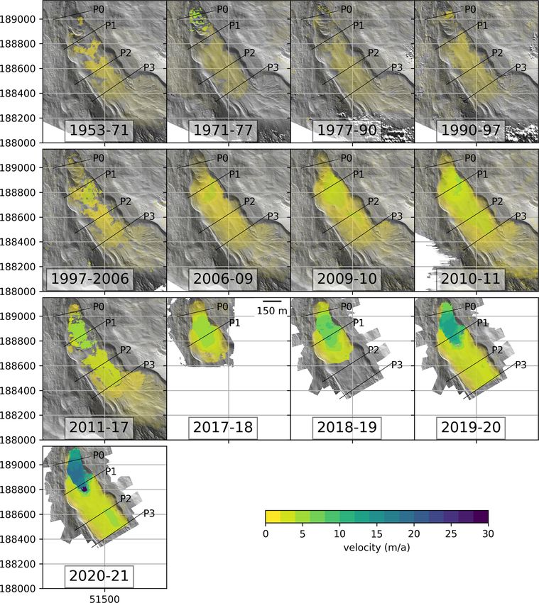
118                                 L. Hartl et al.: Multi-sensor monitoring and data integration reveal cyclical destabilization

1   Introduction                                                    ogy, it is assumed that sliding on shear horizons, which may
                                                                    be basal or located within the structure of the rock glacier,
                                                                    dominates the destabilized movement. In contrast, “normal”
Rock glaciers are lobate or tongue-shaped landforms su-             rock glacier movement is driven by viscous creep of the ice-
persaturated by ice and generated by the former or current          rich permafrost core (Arenson et al., 2002; Roer et al., 2008;
creep of frozen ground (Barsch, 1992; Haeberli et al., 2006;        Krainer et al., 2015; Schoeneich et al., 2015; Marcer et al.,
RGIK, 2022). They are widespread features of the moun-              2019; Cicoira et al., 2019b, 2020). The underlying causes
tain cryosphere and serve as proxies for former and cur-            of destabilization may be climatic (rheological changes due
rent permafrost occurrence, play an important role in the           to increased temperature and/or liquid water input, e.g. De-
hydrological system, and form part of the sediment cas-             laloye et al., 2013), mechanical (local overloading due to
cade (Wahrhaftig and Cox, 1959; Barsch, 1996; Haeberli              rock fall events and subsequent propagation of compressive
et al., 2006; RGIK, 2022). Rock glacier kinematics have             processes, e.g. Scotti et al., 2017), or a combination thereof.
increasingly become of interest during approximately the            We follow the terminology of Marcer et al. (2021) regard-
last 2 decades due to accelerated movement at many rock             ing rock glacier destabilization and refer to their publication
glaciers in the Alps and in creeping subarctic permafrost           for a more comprehensive overview of the conceptual frame-
(Roer, 2005; Delaloye et al., 2008, 2010; Daanen et al.,            work around different phases of destabilization. In the fol-
2012; Kellerer-Pirklbauer et al., 2018; Fleischer et al., 2021).    lowing, we use the term “destabilization signs” to refer to
These general trends are broadly attributed to rising air and       visible morphological features such as scarps, crevasses, and
ground temperatures. However, interannual variations in rock        cracks that develop at the onset of and during destabilization.
glacier velocities often cannot be explained with variations           Relatively little is known about regional distribution of
in mean annual or summer air temperatures alone. This in-           destabilized rock glaciers. Marcer et al. (2019) find evidence
dicates a multifaceted and scale-dependent relationship be-         of destabilization at 10 % of active rock glaciers in France
tween climate forcing and rock glacier response (Delaloye           based on topographic data from 2000 to 2013. Interestingly,
et al., 2008, 2010; Sorg et al., 2015; Hartl et al., 2016b;         they note that destabilizing rock glaciers tend to be pebbly as
Kellerer-Pirklbauer et al., 2017; Müller et al., 2016; Cicoira      opposed to bouldery (Ikeda and Matsuoka, 2006) and located
et al., 2019a; Fleischer et al., 2021). Sub-seasonal monitor-       in densely jointed lithologies (i.e. ophiolites and schists) as
ing of rock glacier movement has shown correlations be-             opposed to crystalline lithologies. Expanding their analysis
tween short-term velocity fluctuations and water input from         further into the past, Marcer et al. (2021) identify a small
snowmelt or precipitation. Liquid water within the rock             number of rock glaciers in France that experienced a form of
glacier strongly affects the material properties relevant to the    destabilization around the middle of the 20th century. These
rheology and hence kinematics of the moving mass (Krainer           rock glaciers then returned to normal behaviour and began
and He, 2006; Wirz et al., 2016; Kenner et al., 2017; Buchli        destabilizing once again in the last 2 to 3 decades. Case stud-
et al., 2018; Cicoira et al., 2019b; Fleischer et al., 2021).       ies have detailed the destabilization of rock glaciers through-
   In recent years, the term “destabilization” has gained trac-     out the Alps in Switzerland, France, Italy, and Austria (Avian
tion in the context of rock glacier acceleration. While there       et al., 2005; Delaloye et al., 2013; Scotti et al., 2017; Vivero
is no universal, exact definition of rock glacier destabiliza-      and Lambiel, 2019; Kaufmann et al., 2021; Bearzot et al.,
tion to date, it is generally understood to mean anomalous          2022; Vivero et al., 2022). While not all accelerating rock
“landslide-like behaviour” (Marcer et al., 2021). Destabiliza-      glaciers are necessarily destabilized, pronounced or unusual
tion is characterized by a sudden, strong, and often localized      acceleration patterns may hint at destabilization processes
increase in velocity and the concurrent appearance of mor-          at the respective sites. This applies to the Alps, as well as
phological destabilization signs like cracks, crevasses, and        other mountain regions, even though related studies do not
scarps (Roer, 2005; Roer et al., 2008; Delaloye et al., 2013).      always explicitly use the term destabilization to describe the
Destabilization appears to require favourable terrain, i.e. a       observed changes (Delaloye et al., 2010; Daanen et al., 2012;
relatively steep slope angle, and onset often occurs at convex-     Hartl et al., 2016b; Eriksen et al., 2018; Kääb et al., 2021).
ities or terrain steps (Marcer et al., 2019, 2021). Velocity dis-      In most cases, destabilization is followed by degradation
continuities and morphological destabilization signs develop        (Cicoira et al., 2020), i.e. deceleration and eventual inactiv-
in these areas, and the rock glacier is essentially split into a    ity of the previously destabilized section of the rock glacier.
destabilized (usually lower) section and a comparatively un-        In rare cases, the complete collapse of the destabilized sec-
affected (usually upper) section (Cicoira et al., 2020). Desta-     tion followed by a rapid mass movement of substantial parts
bilization features like crevasses and deep cracks allow rain       of the affected rock glacier has been observed. Such events
or meltwater to enter the rock glacier, further contributing to     tend to be preceded by high temperatures and wet conditions
acceleration and changes in rheology and kinematics (Roer,          caused by, e.g. significant individual precipitation events,
2005; Delaloye et al., 2013; Buchli et al., 2018; Eriksen           longer periods with anomalous amounts of precipitation, or
et al., 2018; Vivero and Lambiel, 2019). In terms of rheol-

Earth Surf. Dynam., 11, 117–147, 2023                                                https://doi.org/10.5194/esurf-11-117-2023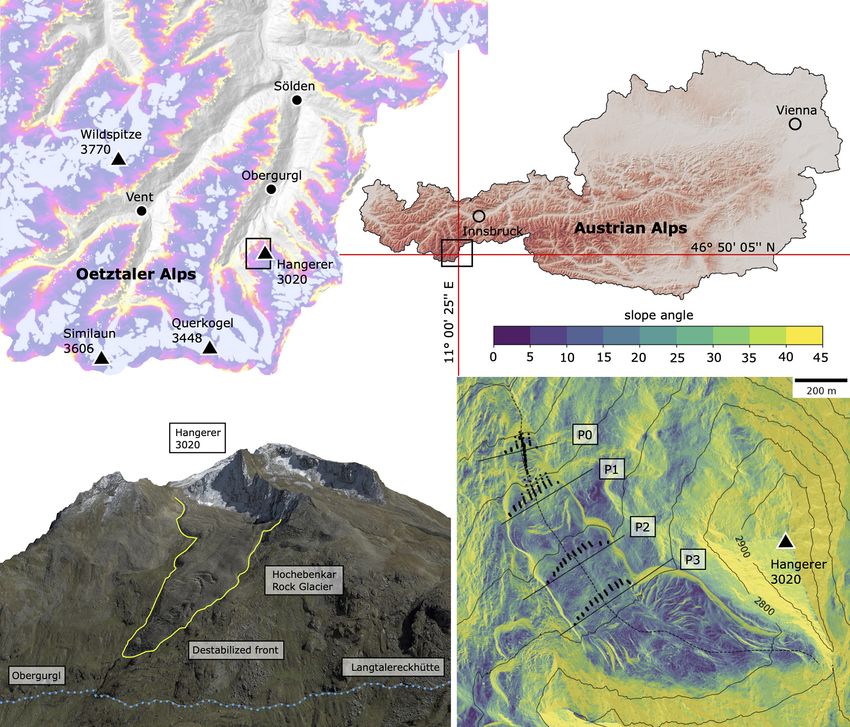
L. Hartl et al.: Multi-sensor monitoring and data integration reveal cyclical destabilization                                  119

water input through snowmelt. Morphological destabiliza-            metres (up to > 10 m) thick surface layer of ice-free, coarse
tion signs prior to the collapse have been reported in cases for    debris (Nickus et al., 2015; Hartl et al., 2016a). It should be
which detailed analyses of collapse events exist (Krysiecki         noted that the depth of the bedrock is not necessarily the
et al., 2008; Bodin et al., 2012, 2017; Marcer et al., 2020;        same as the thickness of the moving mass or the thickness
Kofler et al., 2021). At some sites, e.g. Grabengufer rock          of the thermally defined permafrost within the rock glacier.
glacier in Switzerland, the combination of very high veloci-        The surface debris has an average grain size of 35 to about
ties, obvious signs of destabilization, and downstream topog-       60 cm, with some blocks reaching diameters of up to a few
raphy favourable for mass movements led to concern but did          metres (Nickus et al., 2015). A layer of finer material below
not produce debris flows (Delaloye et al., 2013). This sug-         the coarse surface debris is exposed at the steep frontal slope
gests that the underlying processes are complex and depend          of the rock glacier. The surrounding lithology is part of the
on a variety of internal (composition of the rock glacier, inter-   crystalline Ötztal–Stubai complex, and the bedrock is com-
nal hydrological processes) and external (meteorological and        posed mainly of paragneiss and mica schists (Nickus et al.,
climatological forcing, surrounding terrain) factors (Marcer        2015).
et al., 2019, 2021).                                                   Surveys of the temperature at the bottom of the winter
                                                                    snow cover (BTS) carried out in 1976 (Haeberli and Patzelt,
1.1   Äußeres Hochebenkar rock glacier
                                                                    1982) and 2010 indicate a reduction in the extent of the dis-
                                                                    continuous permafrost surrounding the rock glacier during
In the following, we present data from an interdisci-               this period, particularly at the margins of the rock glacier
plinary monitoring network at the rock glacier in Äußeres           and directly below the terminus (Nickus et al., 2015). This
Hochebenkar (HEK) in the Austrian Alps (Fig. 1) and dis-            is in line with the overall degradation of ground ice in the
cuss the behaviour of the lower section of the rock glacier         Alps as reported by, e.g. Etzelmüller et al. (2020). The rock
through the lens of destabilization. HEK is a fast-moving,          glacier terminus was at the lower end of the discontinu-
tongue-shaped talus rock glacier with a long history of sci-        ous permafrost margin even in the 1970s and has advanced
entific study (Table 1). It is one of 556 intact rock glaciers in   downwards since, hence moving further below the likely per-
the Ötztal mountain range (Wagner et al., 2020) and covers          mafrost margin. The permafrost index map of Boeckli et al.
an area of about 0.4 km2 . The root zone reaches a maximum          (2012b) suggests that permafrost is relatively likely in the
elevation of about 2870 m and the terminus currently extends        upper parts of HEK, but this is likely the case only under
down to about 2370 m. Note that, unless otherwise specified,        cold or very favourable conditions near the terminus. Zahs
all elevation values in this paper refer to orthometric heights     et al. (2019) found no permafrost in an electrical resistivity
(EVRF2000 Austria height, EPSG:9274). The slope angle of            tomography (ERT) profile beside the rock glacier at an eleva-
the rock glacier is moderate in the upper section and steepens      tion of about 2470 m. In a profile at a similar elevation on the
below a terrain step at around 2570 m. The terminus funnels         rock glacier terminus they reported resistivities indicative of
into a drainage gully, which is located directly above an ac-       ice-rich frozen ground with variable ice content.
cess road leading to mountain huts further up the valley. The          Regular measurements of block displacements on the sur-
road has recently been affected by rock fall from the rock          face of the HEK rock glacier began in the early 1950s and
glacier terminus and is threatened by any further destabiliza-      continue to this day. Since the 2000s, numerous remote-
tion.                                                               sensing-based studies have used a variety of methods and
   Climatologically, HEK is located in a relatively dry, inner-     analysis techniques to quantify surface elevation change and
alpine valley. The mean annual air temperature (MAAT) in            horizontal displacement at HEK, providing spatial context
nearby Obergurgl (1938 m a.s.l.) was 2.2 ◦ C during the 1961–       to the in situ monitoring of block movement. Summarizing
1990 reference period and 2.7 ◦ C during the 1991–2020 ref-         broadly, previous studies show that vertical surface elevation
erence period (Kuhn et al., 2013). Mean annual precipitation        changes are typically small or slightly negative in the upper
sums at the Obergurgl weather station were between about            part of the rock glacier, while the lower section is extending
840 and 900 mm depending on the reference period (data              downwards and thinning. See Table 1 for an overview of the
obtained from ZAMG data hub, https://data.hub.zamg.ac.at/,          respective literature.
last access: 23 February 2023, Dautz et al., 2022). Mete-              Morphological observations in early studies and the long
orological data from an automatic weather station at HEK            time series of block velocities indicate processes of desta-
(2565 m a.s.l.) show that MAAT at the rock glacier was close        bilization at HEK in the 1950s and 1960s. During surveys
to 0 ◦ C in recent years (Stocker-Waldhuber et al., 2013).          in the 1970s, Haeberli and Patzelt (1982) observed large
   Using refraction seismics, Haeberli and Patzelt (1982)           crevasses in the lowest section of the rock glacier tongue.
found the mean thickness of the rock glacier to be about 40 m       They noted one crevasse crossing the entire width of the
and estimated an ice content of 50 %. More recent ground-           rock glacier at around 2540 m and speculated that the low-
penetrating radar (GPR) surveys found comparable values             est section of the terminus below this crevasse had previ-
for the mean depth of the bedrock, with considerable vari-          ously undergone a process of separation or decoupling from
ation in depth throughout the rock glacier area, and a several      the upper part. Schneider and Schneider (2001) interpreted

https://doi.org/10.5194/esurf-11-117-2023                                               Earth Surf. Dynam., 11, 117–147, 2023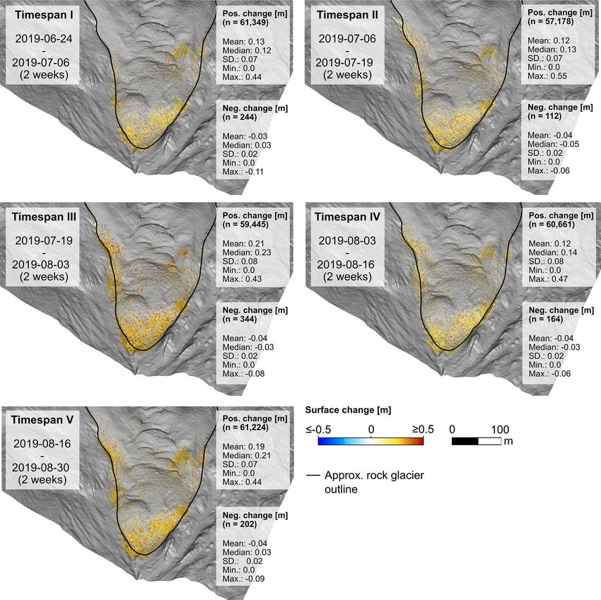
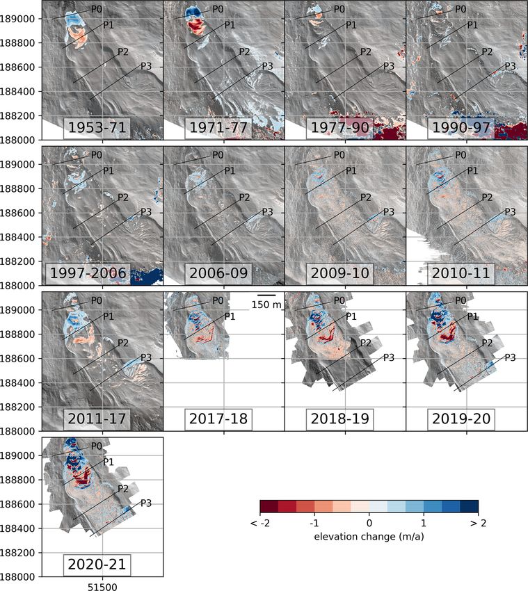
120                                  L. Hartl et al.: Multi-sensor monitoring and data integration reveal cyclical destabilization

Figure 1. Location of the study area in the Austrian Alps (top right, red shading shows elevation; base data: NASA Shuttle Radar Topography
Mission (SRTM)) and detail of the geographical context of the Hochebenkar rock glacier in the Ötztal Alps (top left; base data: SRTM): the
overlay shows the permafrost index map as per Boeckli et al. (2012a), light blue indicates a glacier, dark blue indicates permafrost in nearly
all conditions, purple indicates permafrost mostly in cold conditions, and yellow indicates permafrost only in very favourable conditions.
A 3D visualization of the study site (bottom left; base data: SRTM and © Google Earth) and slope angle map draped over hillshade with
contour lines, which have all been generated from the 2017 digital surface model (bottom right). Black dots mark the positions of the blocks
in the four cross profiles and the longitudinal profile for 2015–2021. Also shown are the central flowline (dashed black line) and the lines
between the fixed reference points that define the positions of the cross profiles (solid black lines).

the kinematics of the lower section of the rock glacier in               as opposed to the permafrost creep governing the upper sec-
a similar manner, agreeing with the idea that the terminus               tion, describing the same general destabilization processes as
area had separated from the main body of the rock glacier.               more recent work (Roer et al., 2008; Schoeneich et al., 2015;
They described the main part as being in a normal state (Nor-            Marcer et al., 2019; Cicoira et al., 2020).
malzustand) and healthy (gesund), whereas the behaviour of                  After this early period of high velocities and destabiliza-
the presumably separated part was considered extraordinary               tion, the rock glacier returned to its “normal” state until the
(außergewöhnlich). Schneider and Schneider (2001) further                onset of a second phase of acceleration in the mid-1990s.
hypothesized that the process of separation of the entire sec-           The lower section below the terrain step and the crevasse ob-
tion below the terrain step was completed by the early 1970s             served by Haeberli and Patzelt (1982) also accelerated again
and that it might repeat in the future given continued ad-               with a peak in velocities in 2004 and a stronger and currently
vancement of the rock glacier over the terrain step. They                ongoing acceleration after 2010 (Hartl et al., 2016b).
speculated that the lowest section of the terminus became
inactive after this destabilization phase due to the loss of ice-
rich permafrost in the terminus area. Schneider and Schnei-              1.2    Objectives
der (2001) attributed the anomalous behaviour in the lower               Our overarching goal is to contribute to the developing sci-
section to the steep slope angle and basal sliding processes             entific discussion around rock glacier destabilization by con-

Earth Surf. Dynam., 11, 117–147, 2023                                                       https://doi.org/10.5194/esurf-11-117-2023
L. Hartl et al.: Multi-sensor monitoring and data integration reveal cyclical destabilization                                                  121

Table 1. Overview of previous studies at HEK rock glacier, grouped by thematic focus and listed chronologically per thematic group.

  Interdisciplinary overview publications
  Permafrost mapping based on a bottom of the winter snow cover (BTS) survey, descriptions        Haeberli and Patzelt (1982)
  of morphological features on the rock glacier surface, and refraction seismics.
  Geological setting, BTS data, presentation of first ground-penetrating radar (GPR) survey,      Nickus et al. (2015)
  streamflow data, and analysis of conductivity and chemical composition of rock glacier
  runoff.
  Displacement of block profiles
  Details on establishment of block profiles and the first ∼ 2 decades of measurements.           Vietoris (1958, 1972), Pillewizer (1957)
  Digitization of early data, homogenization of time series, systematic assessment of mean        Schneider (1999a, b)
  profile velocities and single blocks, and analysis of surface elevation change at the block
  locations.
  Overview of block movement since the beginning of measurements and consolidation of             Schneider and Schneider (2001)
  results of Schneider (1999a, b) and considerations on the role of climate parameters as
  drivers of block movement.
  Update to time series of block profiles, including profile 0 (established in 1997), and sta-    Hartl et al. (2016b)
  tistical analysis of the correlation between cumulative anomalies of movement and annual
  and seasonal means of climate parameters.
  Remote sensing
  Terrestrial photogrammetric surveys of the rock glacier tongue (advance of 1.1 m between        Vietoris (1972)
  1953–1955 at the main, orographic left lobe); no movement is detected at the smaller, oro-
  graphic right lobe for 1956–1966 (unpublished data cited in Vietoris, 1972)
  Terrestrial photogrammetric surveys of the lower section of the rock glacier in 1986, 1999,     Kaufmann and Ladstädter (2002b, a),
  2003, and 2008 and detailed analysis thereof; computation of 3D flow vectors; and an            Ladstädter and Kaufmann (2005),
  overview and analysis of historic cartographic and photogrammetric data.                        Kaufmann (2012)
  Analysis of orthophotos to generate digital surface models (DSMs) and horizontal flow           Klug (2011), Klug et al. (2012)
  vectors (orthophotos available for 1953, 1969, 1971, 1977, 1990, and 1997).
  Analysis of airborne laser scanning (ALS) data to generate digital elevation model and flow     Bollmann et al. (2012), Klug et al. (2012)
  vectors (ALS data for 2006, 2009, 2010, and 2011).
  Multi-source – ALS, terrestrial laser scanning (TLS), uncrewed aerial vehicle (UAV)-borne       Zahs et al. (2019, 2022a, b), Ulrich et al.
  laser scanning (ULS), and UAV-borne photogrammetry-based dense image matching (DIM)             (2021)
  – 3D topographic change analysis for different time spans in the period 2006–2021, includ-
  ing bi-weekly monitoring in summer 2019.
  Geophysics
  Refraction seismics with surveys carried out in 1975 and 1977, with a mean ice content of       Haeberli and Patzelt (1982)
  about 50 % at surveyed profiles.
  Ground-penetrating radar with surveys carried out in 2000, 2008, and 2013 with two differ-      Nickus et al. (2015), Hartl et al. (2016a)
  ent radar systems at different locations on the rock glacier, with a mean depth of bedrock
  between 34 and 45 m depending on survey year.
  Electrical resistivity tomography with a survey carried out in 2016 at two profile lines next   Zahs et al. (2019)
  to and on the margin of the rock glacier tongue, with no indications of permafrost beside
  the rock glacier, and isolated ice lenses identified in the profile on the tongue.

solidating and making available the in situ and remote sens-               studies and long-term observations (Table 1). Specifically,
ing data basis from our study site. We provide a comprehen-                we perform the following tasks.
sive overview of two separate destabilization periods at the
same rock glacier by combining the most recent multi-sensor
                                                                              – We homogenize and update a time series of 14 digi-
and multi-method monitoring results with data from previous
                                                                                tal surface models (DSMs) derived from aerial imagery

https://doi.org/10.5194/esurf-11-117-2023                                                         Earth Surf. Dynam., 11, 117–147, 2023
122 L. Hartl et al.: Multi-sensor monitoring and data integration reveal cyclical destabilization
(1953–1997; Klug, 2011) and lidar point clouds, also of the kinematics of HEK rock glacier up to 2015. Histori-
referred to as laser scanning (2006–2021). cally, reporting focused on mean displacement values for the
cross profiles P0, P1, P2, and P3. The mean value was com-
– We present the most recent data from the long-term in puted as the arithmetic mean of all blocks in the profile, and
situ time series of differential global navigation satel- displacement refers to the absolute, three-dimensional dis-
lite system (DGNSS)-based block displacement, updat- tance moved. Given issues related to averaging and changing
ing the dataset presented in Hartl et al. (2016b) (time numbers of blocks in the profiles, Hartl et al. (2016b) esti-
series: 1952–2022). mate an uncertainty of between ±0.2 and ±0.5 m a−1 for the
mean profile velocities. We adhere to the same method of us-
– We compute a time series of the bulk creep factor (BCF)
ing 3D trajectories of single blocks as part of a profile when
as a metric of destabilization (Cicoira et al., 2020) to aid
referring to profile means in order to be consistent with the
interpretation of velocity change.
long-term time series. Measurements are carried out annually
– We extract additional information about the rock in summer, usually in late August or early September. Annual
glacier’s recent surface change from very high- mean values are derived from the absolute displacement and
resolution (centimetre point spacing) 3D point clouds. the number of days between measurement campaigns. The
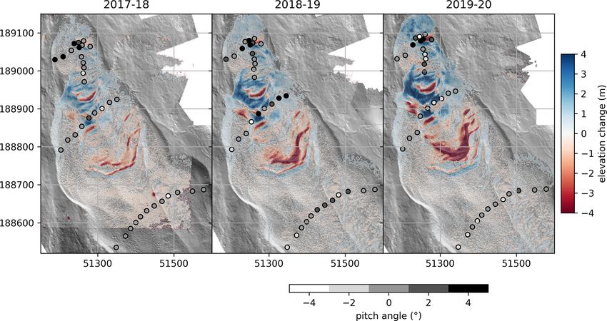
We derive (a) 3D change information between two tachymeter and DGNSS displacement measurements for sin-
epochs based on corresponding planar boulder faces at gle blocks are considered accurate to ±3 cm vertically and
the rock glacier front (Zahs et al., 2022a, b) and (b) a horizontally (Niederwald, 2009; Nickus et al., 2015). In the
time series of rotating single blocks. 2021–2022 measurement year, multiple marked blocks in P1
were lost due to the rapid movement of the rock glacier in
Following an overview of the different datasets and meth- this area. We present velocities for the remaining blocks in
ods, the results are structured chronologically, moving from the profile for the most recent measurement year but do not
the first period of destabilization to the subsequent “stable” compute a mean profile velocity, as this would no longer be
period and the start of the ongoing renewed acceleration and representative given the lost blocks. We refer to the exist-
destabilization. For each period, we describe kinematic and ing literature for further details on the time series of block
morphological changes based on the in situ and remote sens- displacement (see Table 1; Schneider and Schneider, 2001;
ing datasets. For the most recent years, we present additional Niederwald, 2009; Hartl et al., 2016b).
results based on the fusion of high-resolution laser scanning The dynamics of destabilized rock glaciers are character-
data and block displacement, as well as data on sub-seasonal ized by velocity discontinuities between the faster, destabi-
3D topographic change at the rock glacier front for the sum- lized (usually lower) section and the slower, non-destabilized
mer of 2019. In the Discussion, we then consider uncertain- (usually upper) section. As this discontinuity becomes more
ties and limitations related to the different datasets and meth- pronounced under ongoing destabilization, the surface strain
ods and offer an interpretation of the observed changes in the between the two sections also increases (Marcer et al., 2021).
general context of rock glacier destabilization. Hence, changes in surface strain rates can serve as indica-
tors of destabilization onset in specific sections of a rock
glacier. To quantify these changes for recent years at HEK,
2 Data and methods
we use the positions of individual blocks in P1 and P2 to
2.1 Long-term geodetic surface displacement
compute surface strain rates across the terrain step and the
monitoring
velocity discontinuity located between P1 and P2, i.e. be-
tween the currently destabilized lower section and the non-
Since 1954, surface displacement of HEK rock glacier has destabilized upper section. The surface strain rate between a
been measured geodetically along three cross profiles (Vi- pair of blocks (b1, b2) in P1 and P2 is given by the differ-
etoris, 1958, 1972). See Fig. 1 for an overview of the profile ence in velocity between b1 and b2 divided by the distance
locations. Measurements were initially carried out annually, between b1 and b2, following Marcer et al. (2021).
but the time series has substantial gaps from the 1960s un-
til 1997, when a fourth cross profile and a longitudinal profile 2.2 Meteorological data
were installed in the lowest section and the monitoring efforts
were revitalized (Fig. 2). Schneider (1999a, b) Schneider and As part of the HEK monitoring network, an automatic
Schneider (2001), and Niederwald (2009) give details on the weather station (AWS) was installed at 2565 m in 2010 di-
homogenization of the time series and early measurement rectly beside the rock glacier (Stocker-Waldhuber et al.,
techniques. Since 2008, displacement measurements have 2013; Hartl and Fischer, 2015). Long-term meteorological
been carried out with a Topcon Hiper Pro real-time kine- data have been available from a semi-automatic weather sta-
matic DGNSS, replacing a theodolite and tachymeter pre- tion in Obergurgl since 1953. This station is located about
viously used for the same purpose. Hartl et al. (2016b) de- 4 km down the valley from the rock glacier. From 1953
scribe the current measurement system and give an overview to 1998 the Obergurgl station was located at 1938 m a.s.l. It
Earth Surf. Dynam., 11, 117–147, 2023 https://doi.org/10.5194/esurf-11-117-2023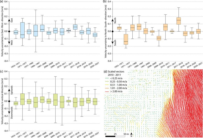
L. Hartl et al.: Multi-sensor monitoring and data integration reveal cyclical destabilization                                      123

Figure 2. Overview of datasets used in this study: DSMs, orthophotos, and TLS data as detailed in Table 2. DGNSS monitoring refers to in
situ geodetic monitoring of block displacement.

was then moved to a nearby location at 1941 m a.s.l. Data             the middle part of the rock glacier. All acquisitions followed
are available from the data portal of the Austrian Central In-        the same flight plan: aside from small connection lines, the
stitution for Meteorology and Geodynamics (ZAMG, https:               rock glacier was captured by a set of parallel flight lines
//data.hub.zamg.ac.at/, last access: 23 February 2023), which         with a horizontal spacing of 100 m, oriented perpendicular
operates the station (Dautz et al., 2022). An overview of the         to the flow direction of the rock glacier. The average flying
meteorological time series from the Obergurgl station can be          height above ground level (AGL) was between 70 and 120 m.
found in Kuhn et al. (2013).                                          The flight speed was 8 m s−1 , the pulse repetition rate (PRR)
                                                                      was 820 kHz, and the angular resolution was 0.0476◦ . Fol-
2.3     Remote-sensing-based area-wide monitoring of                  lowing standard procedures, such as flight trajectory post-
        topographic change                                            processing, point extraction, geo-referencing, and strip ad-
                                                                      justment, the resulting point clouds were co-registered to the
Table 2 and Fig. 2 give an overview of all topographic data           ALS 2017 dataset by using the iterative closest point algo-
used for this study, which includes 14 DSMs covering a time           rithm (ICP) algorithm to minimize distances between the
period of 68 years, as well as orthophotos from UAV surveys           point clouds in stable areas of bedrock outcrops. For details
and TLS-based point clouds of the front and lower termi-              on the 2017 dataset used as reference, please see Table 2
nus area. Photogrammetrically reconstructed surface topog-            and Rieger (2019). In addition to the processed point clouds,
raphy based on historical analogue aerial imagery is avail-           0.1 and 1 m resolution DSMs and 3 cm resolution orthopho-
able for multiple years between 1953 and 1997. Please see             tos were created.
Klug (2011) for details on the aerial imagery and related pro-           To quantify sub-seasonal changes at the rock glacier front
cessing steps. In more recent years, various airborne laser           and lower terminus, a bi-weekly (24 June to 30 August)
scanning (ALS), terrestrial laser scanning (TLS), and UAV-            time series of six terrestrial laser scanning (TLS) point
based laser scanning (ULS) surveys were carried out at HEK.           clouds was captured in 2019. This temporally highly re-
We describe the ULS data acquisition set-up and give de-              solved dataset complements an annual TLS time series start-
tails on the processing of the TLS datasets in Sect. 2.3.1.           ing in 2015 and described in Ulrich et al. (2021) and Zahs
In Sect. 2.3.2, we describe the work flow used to create a            et al. (2022a). We refer to these publications for more de-
homogenized time series of DSMs that combines the pho-                tailed information on the TLS data acquisition and measure-
togrammetrically reconstructed surface topography (Klug,              ment set-up. Bi-weekly change in 2019 was computed us-
2011) and the recent ALS and ULS datasets. We further de-             ing the correspondence-driven plane-based M3C2 (CD-PB
scribe time series of surface velocity and elevation change           M3C2) algorithm (Zahs et al., 2022b). The CD-PB M3C2
that were derived from the DSMs. Finally, in Sect. 2.3.3              reduces uncertainty in the quantification of low-magnitude
we describe how rotational information for individual blocks          (< 0.1 m) 3D topographic change. Thus, it allows confident
was computed from a combination of ULS point clouds and               detection of small changes in natural landscapes with com-
results of the DGNSS monitoring.                                      plex surface dynamics, i.e. locally planar but overall rough
                                                                      morphology. To derive 3D change between two epochs t1
2.3.1    Recent high-resolution monitoring of                         and t2, the algorithm computes the distance between corre-
         3D topographic change                                        sponding planar areas (plane pairs). Change is thereby com-
                                                                      puted along the normal vector of the plane in t1. When ap-
In 2018, 2019, 2020, and 2021, ULS campaigns were con-                plied to rock glaciers, the method can make use of the sur-
ducted with a Riegl RiCopter UAV, carrying a VUX-1LR                  face of a rock glacier being most planar at the scale of faces
kinematic laser scanner, run with a 336◦ field of view and            of individual boulders. These boulders move with the general
combined with an Applanix AP20 inertial measurement                   creep of the rock glacier rather than independently and can
unit (IMU) (Bremer et al., 2019). Additionally, a nadir-              be re-identified in successive epochs due to their moderate
looking Sony Alpha 6000 RGB camera was mounted for or-                magnitudes of movement at the monitored interval (Ulrich
thophoto creation. In 2018, only the lower terminus area was          et al., 2021). We used these corresponding planar boulder
captured. The following flight campaigns were extended to

https://doi.org/10.5194/esurf-11-117-2023                                                  Earth Surf. Dynam., 11, 117–147, 2023
124                                                   L. Hartl et al.: Multi-sensor monitoring and data integration reveal cyclical destabilization

Table 2. Metadata for the presented topographic data. Values for differential digital surface model (DDSM) uncertainty and level of detection
refer to the DDSM or DSM pair of the given and previous year, respectively (in m a−1 ).

                                                                         Long-term time series of topographic change
   Acquisition date            Data source                                  Spatial coverage            DDSM uncertainty            Level of                          Reference
                                                                                                         (i.e. 2.5 %/97.5 %         detection for
                                                                                                                quantiles of        velocities (i.e.
                                                                                                                   elevation        median velocities
                                                                                                                  difference        in stable
                                                                                                                    in stable       areas in x/y/z
                                                                                                                   outcrops)        directions)
   31 Aug 1953                 Aerial photographs (analogue                 Entire rock glacier                                                                       Klug (2011)
                               aerial stereoscopic pairs, Fed-
                               eral Office of Metrology and
                               Surveying, BEV)
   18 Aug 1971                 Aerial photographs (analogue                 Entire rock glacier              −0.07/ + 0.08          −0.01/0.04/ − 0.03                Klug (2011)
                               aerial stereoscopic pairs, BEV)
   7 Sep 1977                  Aerial photographs (analogue                 Entire rock glacier              −0.21/ + 0.17          −0.03/ − 0.16/0.03                Klug (2011)
                               aerial stereoscopic pairs, BEV)
   10 Oct 1990                 Aerial photographs (analogue                 Entire rock glacier              −0.11/ + 0.12          0.01/0.03/ − 0.01                 Klug (2011)
                               aerial stereoscopic pairs, BEV)
   11 Sep 1997                 Aerial photographs (analogue                 Entire rock glacier              −0.18/ + 0.21          −0.01/0.05/ − 0.01                Klug (2011)
                               aerial stereoscopic pairs, BEV)
   23 Aug 2006                 ALS flight campaign, govern-                 Entire rock glacier              −0.19/ + 0.13          0.04/ − 0.01/0.02                 Land    Tirol  Abteilung
                               ment of Tyrol                                                                                                                          Geoinformation
                                                                                                                                                                      (2011, 2019)
   9 Sep 2009                  ALS flight campaigns carried                 Entire rock glacier              −0.13/ + 0.18          −0.01/0.00/0.00                   Bollmann et al. (2012),
                               out within the ACRP (Austrian                                                                                                          Klug et al. (2012)
                               Climate Research Programme)
                               project C4AUSTRIA (project
                               no. 384 A963633)
   9 Oct 2010                  ALS flight campaigns car-                    Entire rock glacier                  −0.33/0.31         0.01/ − 0.09/0.02                 Roncat et al. (2013a, b)
                               ried out within the project
                               MUSICALS           (Multiscale
                               Snow/Icemelt Discharge Sim-
                               ulation for Alpine Reservoirs,
                               alpS/COMET)
   3 Oct 2011                  ALS flight campaigns carried                 Entire rock glacier              −0.33/ + 0.35          −0.01/0.06/ − 0.01                Bollmann       et     al.
                               out within the ACRP (Austrian                                                                                                          (2012, 2015), Zahs et al.
                               Climate Research Programme)                                                                                                            (2019)
                               project C4AUSTRIA (project
                               no. 384 A963633)
   15 Sep 2017                 ALS flight campaign, govern-                 Entire rock glacier              −0.06/ + 0.06          0.01/0.00/0.00                    Land     Tirol Abteilung
                               ment of Tyrol                                                                                                                          Geoinformation   (2011),
                                                                                                                                                                      Rieger (2019)
   30 Jul 2018                 ULS                                          Terminus                         −0.16/ + 0.28          0.07/0.15/ − 0.02                 This study
   30 Aug 2019                 ULS                                          Lower section                    −0.21/ + 0.11          0.00/ − 0.04/ − 0.01              This study
   18 Sep 2020                 ULS                                          Lower section                    −0.09/ + 0.08          0.00/ − 0.02/ − 0.01              This study
   13 Aug 2021                 ULS                                          Lower section                    −0.07/ + 0.16          −0.04/ − 0.01/ − 0.01             This study
                                                                                               Other data
   2019, bi-weekly             TLS                                          Terminus                       Alignment error          –                                 Zahs et al. (2022a, b)
   during the summer                                                                                         between point
                                                                                                                   clouds:
                                                                                                           0.011–0.013 m∗
   18 Sep 2020                 UAV orthophotos                              Lower section                                     –     –                                 This study
   13 Aug 2021                 UAV orthophotos                              Lower section                                     –     –                                 This study
  ∗ Alignment error is assessed by calculating the standard deviation of M3C2 distances on stable bedrock outcrops distributed around the rock glacier (Fey and Wichmann, 2017; Zahs et al., 2022a).

Earth Surf. Dynam., 11, 117–147, 2023                                                                                                   https://doi.org/10.5194/esurf-11-117-2023
L. Hartl et al.: Multi-sensor monitoring and data integration reveal cyclical destabilization                                   125

faces for change analysis of the rock glacier front and lower       windows), providing a controlled subsampling of the raster
terminus between the epochs. Change analysis was carried            data while enhancing the computational efficiency. Displace-
out in the flow direction of the rock glacier, in the vertical      ment vectors were then derived based on the detected posi-
direction, and in the horizontal direction. The CD-PB M3C2          tional shifts of the reference patterns. The IMCORR algo-
algorithm additionally estimates the uncertainty associated         rithm uses the shaded reliefs and the DSMs for the 2D pat-
with quantified change. It therefore allows confident anal-         tern matching so that a vertical displacement component can
ysis of change by separating significant change (magnitude          be added. Hence, the final output of the IMCORR analy-
of change > uncertainty) from non-significant or no change          sis was 2.5D displacement vectors covering the active rock
(magnitude of change ≤ uncertainty).                                glacier and surrounding stable areas for each pair of subse-
                                                                    quent DSMs. The total area covered varies for each survey
2.3.2   Long-term change monitoring
                                                                    campaign (Table 2).
                                                                       Mean annual velocities (m a−1 ) between the individual
The photogrammetrically reconstructed topography and the            epochs were calculated by dividing the 2.5D displacement
3D point clouds derived from ALS and ULS were co-                   vector lengths by the respective time period. The result-
registered within bedrock outcrops assumed to be sta-               ing vectors of mean annual velocity were filtered semi-
ble throughout the established time series. For the co-             automatically to only consider downslope movement and re-
registration, the ICP (Besl and McKay, 1992) was used, im-          move minor outliers in stable areas. To allow a comparison
plemented in C++ in an extension of the SAGA GIS soft-              with the results of the DGNSS monitoring, the mean veloc-
ware (Conrad et al., 2015). The 2017 ALS data provided              ities derived from the image correlation analysis were spa-
by the government of the state of Tyrol (Table 2) served            tially aggregated within the movement range of the moni-
as reference for the co-registration. The selected stable ar-       tored blocks (area around the block positions as shown in
eas are distributed across the study area and include varying       Fig. 1).
slope angles and orientations in order to reach a robust co-           As an uncertainty assessment, the east–west and north–
registration. Due to the topography of the cirque in which the      south components of the velocity vectors on stable ground
rock glacier is located, only relatively small parts of the study   were analysed individually for each period. The result of this
area have slopes, oriented mainly to the north and south, and       is an uncertainty estimate for the velocity vector field over
minor shifts of the registration in a north–south direction can-    the rock glacier in the east–west and north–south direction
not be ruled out. The implications of this are discussed in         for each period. On the rock glacier surface, displacement
Sect. 4.1.                                                          vectors show a uniform direction due to the movement of the
   After co-registration, DSMs with a spatial resolution of         rock glacier (Fig. 3, box 1). In contrast, pattern shifts on sta-
1 m were computed for each epoch of the multi-temporal              ble ground outside of the rock glacier are minor, and the de-
point clouds by aggregating the average elevation of all            rived velocity vectors are small and mostly show arbitrary di-
points per raster cell. This 1 m resolution matches the res-        rections (Fig. 3, box 2). Arbitrary directions of vectors on sta-
olution of the DSMs previously derived from aerial imagery          ble ground indicate random noise in the data, whereas a non-
(Klug, 2011). The DSMs computed from the digitized ana-             random distribution of vectors on stable ground indicates
logue images do not include the same level of topographic           higher errors, e.g. due to shifts in the registration. The fo-
detail as the DSMs derived from laser scanning. In some             cus of this study is on the velocity of the rock glacier; hence,
cases, the images have localized shading effects in the steeper     the uncertainty analysis is centred on this aspect. Please see
sections of the terminus, which produces gaps in the topo-          the references in Table 2 for more detail on absolute uncer-
graphic information extracted from the images. Please see           tainties of the underlying topographic data.
Klug (2011) and Klug et al. (2012) for more detailed de-               In order to show patterns of elevation gain and loss, dif-
scriptions of the aerial imagery and the resulting DSMs. All        ferential digital surface models (DDSMs) were computed by
datasets were projected according to the Austria GK West            subtracting the DSMs of two consecutive epochs (Williams,
definition (EPSG:31254, with the vertical datum EVRF2000            2012). DDSM uncertainty was assessed by computing the
Austria heights, EPSG:9274).                                        2.5 % and 97.5 % quantile of the elevation difference within
   From the DSMs, shaded reliefs were computed with the             stable bedrock outcrops (Table 2). This provides an estimate
ambient occlusion method (Tarini et al., 2006), prevent-            of the inherent noise and hence the detection threshold for
ing cast shadows. Area-wide displacement vectors were de-           obtaining significant surface changes (Williams, 2012). The
rived with the help of an image correlation technique (IM-          analyses of the multi-temporal DSMs and the displacement
CORR; Scambos et al., 1992). In each pair of subsequent             vectors were conducted with the R statistical programming
datasets, reference patterns within a moving window of the          language (R Core Team, 2021).
first shaded relief (epoch n) were correlated with patterns in
a defined search neighbourhood of the second shaded relief
(epoch n + 1, Fig. 3a). The image correlation was applied at
equally spaced nodes (i.e. central grid cells of the moving

https://doi.org/10.5194/esurf-11-117-2023                                               Earth Surf. Dynam., 11, 117–147, 2023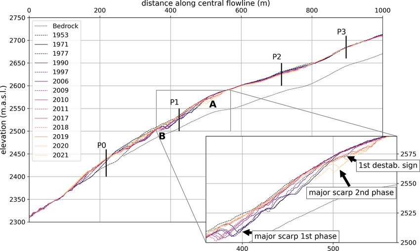
126                                   L. Hartl et al.: Multi-sensor monitoring and data integration reveal cyclical destabilization

Figure 3. Concept of the applied image correlation approach. (a) In the shaded relief of the first epoch n, a box-shaped reference pattern
is analysed for all regularly distributed node positions. The green boxes 1 and 2 are the reference patterns for two example nodes analysed
during this process. For the second epoch n + 1, the reference pattern is matched (dashed box; significant shift for node 1, minor shift
for node 2). (b) The distribution of resulting displacement vectors’ direction in epochs n and n + 1 on the rock glacier at node 1. (c) The
distribution of resulting displacement vectors’ direction between epochs n and n + 1 outside of the rock glacier at node 2. The boxplots in (b)
and (c) present an example of ranges of the derived vector lengths, showing that the uncertainty of the data on stable grounds is only minor
compared to the resulting displacements.

2.3.3   Data fusion approach to generate time series of                     1. We applied an IMCORR image correlation at the cen-
        block rotation                                                         tre position of a given block in the 2021 data using
                                                                               the 0.1 m shaded reliefs of 2021 and 2020 in order to
The movement of destabilized rock glaciers is described
                                                                               reconstruct the position of the block in the previous
as landslide like and may have both translational and rota-
                                                                               epoch (2020). Starting from the resulting 2020 position,
tional components (Buchli et al., 2018; Marcer et al., 2021).
                                                                               the same procedure was repeated to find the 2019 and
While translational movement is relatively well documented
                                                                               2018 positions. For each interval, this led to a 3D trans-
in kinematic rock glacier monitoring, few data on rotational
                                                                               lation vector (x, y, z) describing the estimated block
movement are available. To assess potential rotational move-
                                                                               movement between two epochs.
ment in the recently destabilized section of HEK, we anal-
ysed the rotational movement of individual blocks in the pro-               2. Considering this translation for the initialization of a
file lines. In 2021, the DGNSS measurements of block pro-                      four-by-four transformation matrix, we used the ICP
files and the ULS campaign were conducted only 3 d apart.                      algorithm (implemented in C++ in an extension of
This temporal proximity of the measurements made it pos-                       SAGA GIS, as above) on a block-by-block basis in or-
sible to identify individual blocks from the profiles in the                   der to optimize the alignment of the block shapes be-
ortho-images generated from the 2021 UAV data (resolution:                     tween two consecutive epochs. This was done by a six-
3 cm). Unique block identifiers were manually assigned to                      parameter transformation optimizing translational and
the distinct block shapes in the respective ULS point cloud.                   rotational components. The resulting four-by-four trans-
For each of these selected point ID groups, the following                      formation matrix describes the full-3D transformation
analyses were carried out.                                                     of a block (assumed to be a rigid body).

Earth Surf. Dynam., 11, 117–147, 2023                                                        https://doi.org/10.5194/esurf-11-117-2023
L. Hartl et al.: Multi-sensor monitoring and data integration reveal cyclical destabilization 127
velocities as obtained through the block displacement mea-
surements (Sect. 2.1). The slope angle at each profile is given
by the mean angle along the line between the fixed points
that define the respective profile. The slope angle was ex-
tracted from the DSM time series data (Sect. 2.3.2) resam-
pled to a 10 m × 10 m grid. The resampling to a larger grid
size reduces the influence of variability at the scale of surface
features (such as furrows and ridges or single blocks), which
are not representative of rock glacier geometry in terms of
dynamics. The slope angle between DSM epochs was lin-
Figure 4. Principle of block shape matching in the ULS point early interpolated for years in which DGNSS block measure-
clouds (grey dots) between consecutive time steps (2018–2021). ments are available but DSMs are not. Rock glacier thickness
The iterative closest point (ICP) algorithm was used to match the is given by a map of the rock glacier’s bedrock extrapolated
shape of a block in one epoch onto its shape in another epoch. A from GPR data and presented in Hartl et al. (2016a). This
rotation in the opposite direction of the translation can be recog- is a strong simplification as the depth of the bedrock may
nized for the block shapes. The figure shows examples of downs- differ substantially from the depth of the thermally defined
lope translation and upslope rotation.
permafrost and the thickness of the moving mass. Nonethe-
less, lacking more detailed subsurface information on layer-
3. Finally, the derived matrix allowed decomposition of ing and potential shear horizons, we consider the approxi-
both the translational and rotational components of the mate bedrock depth the best available estimate for our appli-
transformation. For better interpretation, the rotational cation. For parameter calibration, we used the same values
components were derived relative to the translation: the as Cicoira et al. (2020), which were calibrated for a dataset
pitch rotation was defined as being in the same or op- of rock glaciers mostly in the French Alps. This approach
posite direction of translation, and the roll rotation was allows us to directly compare our data with their results.
defined as being around the translation vector (Fig. 4).
2.5 Assessment of geomorphological destabilization
features
2.4 Bulk creep factor The evolution of velocity and elevation change patterns de-
To interpret the observed rock glacier velocities from a dy- rived from the DSM and DDSM time series, along with
namic perspective, we computed the bulk creep factor (BCF) BCF, surface strain rates, and in situ velocity data, can in-
as described by Cicoira et al. (2020). This dimensionless pa- dicate destabilization onset or the end of a destabilization
rameter provides a quantitative basis for the analysis of the period (Marcer et al., 2021). Geomorphological destabiliza-
rheological properties of the rock glacier material, disentan- tion signs – visible changes of surface morphology, such
gling the geometrical component from the velocity signal. as cracks, scarps, and crevasses – are a further indicator of
The calculation of the BCF is based on a modified version destabilization onset. Tracking their appearance and change
of Glen’s flow law (Glen, 1955) adapted for rock glaciers over time in the DSM time series is therefore of interest, par-
(Arenson and Springman, 2005; Arenson et al., 2002; Ci- ticularly when considered in combination with other poten-
coira et al., 2020). In the adapted flow law, the strain rates are tial indicators of destabilization. In the following sections,
a function of the rock glacier’s slope angle, thickness, and we consider morphological destabilization signs in conjunc-
mechanical properties. In general terms, high BCF values tion with velocity and elevation changes for each epoch. The
(roughly above 10) indicate destabilized rock glaciers with evolution of particular scarps in zones of the rock glacier
anomalous short-term deformation processes in the shear where destabilization signs repeatedly occur was tracked and
horizon dominating over long-term secondary creep in the visualized throughout the DSM times series by plotting ele-
permafrost material. However, the BCF includes both com- vation profiles along the central flowline. This yields a quan-
ponents (ice-rich core and shear horizon) and remains a titative delineation of scarp depth and downslope movement
proxy value for the heterogeneous properties of rock glacier between epochs, in addition to a qualitative, visual assess-
material, which should be considered in detail for each case. ment of the development of destabilization signs. The geo-
In combination with changes in surface strain rates, spatial morphological analyses are focused particularly on the area
and temporal patterns in surface velocities, and morpholog- around the terrain step at about 2570 m (zone “A”) and a sec-
ical destabilization signs, discontinuities in BCF provide a ond zone with prominent destabilization features lower on
further indication of the onset of a rapid sliding-type move- the terminus (zone “B”) at around 2520 m.
ment.
We computed the BCF for the four cross profiles shown
in Fig. 1 using the time series of the respective mean profile
https://doi.org/10.5194/esurf-11-117-2023 Earth Surf. Dynam., 11, 117–147, 2023128 L. Hartl et al.: Multi-sensor monitoring and data integration reveal cyclical destabilization
3 Results 1999a). The next measurement was carried out in 1970. Be-
tween these two measurements, mean profile velocities de-
3.1 Historical timeline of terminus destabilization creased from 3.9 m a−1 to just under 1.8 m a−1 for P1 and
from 1.5 to 1 m a−1 at P2 (Schneider, 1999a). P3 experienced
The first result we focus on is the updated time series of a slight increase in velocity at the same time as the lower two
surface displacement at HEK and the homogenization and profiles, as well as a slight decrease after 1969–1970. How-
extension of the DSM time series for the site, which now ever, changes were minor and, in contrast to P1 and P2, do
covers a time period of 68 years. We present analyses of not clearly stand out from the later years of the time series.
the multi-temporal DSMs alongside the block displacement P1 shows relatively high BCF values during the 1960s and
measurements. The early data show a destabilization phase early 1970s (up to 12.8), and values at P2 were also elevated.
of the rock glacier from onset to deceleration, with a peak At P3, BCF was only marginally higher during the period of
in the 1960s (Sect. 3.1.1). This is followed by a period of accelerated movement than during the subsequent more sta-
relative stability, which includes the onset of renewed accel- ble period (Fig. 5).
eration in the mid-1990s (Sect. 3.1.2). Detailed data on the From a geomorphological perspective, the first signs of
block profiles for the early years of the time series have been destabilization are already visible in the earliest data. In
presented in previous studies (Schneider, 1999a; Schneider the 1953 DSM, an isolated scarp can be seen at around
and Schneider, 2001; Hartl et al., 2016b). We include the 2580 m a.s.l. (close to zone A in Figs. 7 and 8). In the
mean profile velocities here again in brief to contextualize 1971 DSM, the scarp is a few tens of metres further downhill
the in situ data with the multi-decadal DSM time series and and has notably increased its size in the centre of the rock
morphological observations based on the DSMs. The high- glacier body. Below this area, several other destabilization
frequency and high-resolution 3D data collected in the past signs are visible from 2580 to 2480 m a.s.l. The most promi-
5 years are presented separately in Sect. 3.2. nent scarp (Fig. 7, zone B) appears at about 2520 m a.s.l.,
with a width of more than 150 m across and almost 300 m
3.1.1 First period of destabilization: 1953 to 1977 following the crown. The highest elevation difference is ob-
servable on the orographic left side, with more than 30 verti-
From 1956/1957 onwards, the frozen mass of the rock glacier cal metres between the crown and the top of the destabilized
entered a period of acceleration. Considering the block pro- body. Nearby, several other cracks and scarps are clearly vis-
files (Fig. 5), P1 and P2 arguably showed irregular behaviour ible. In the following years, the destabilization signs rapidly
from the beginning of the respective time series (1955 at P1, change in size and geometry and move downslope. By 1977,
1952 at P2). However, this signal is hard to interpret since the scarp in zone A is almost stable, while the lower area
there are no prior data it can be compared to. Velocity vec- below zone B continues its evolution, especially towards the
tors derived from the 1953 and 1971 DSMs reach values of rock glacier front. A series of profound scarps develop here
1–2 m a−1 in roughly the lower half of the rock glacier, up in a short time span, concurrent with a notable advance of
to the area between P2 and P3 (visible in the velocity vec- the terminus (Figs. 8, 7, and S1 in the Supplement). At the
tor maps in Fig. 6). It should be noted that this DSM pair front, the oversteepened slope shows the last destabilization
does not resolve the terminus well due to shading effects in signs of the first phase with the onset of the lowermost scarp
the underlying aerial imagery. Hence, the DSM pair for this in 1977. In total, the front advanced roughly 115 m ± 10 m
epoch likely does not capture the full range of velocities in horizontally and 50 m vertically between 1953 and 1977. The
the lowest part of the rock glacier. 1953–1971 and 1971–1977 DSM pairs clearly show a pattern
In 1971–1977, velocity vectors of more than 5 m a−1 were of elevation loss below zone B and concurrent elevation gain
recorded at the terminus. In the upper part of the rock glacier, at the lowest end of the advancing terminus (Fig. 9).
the measurements show a decrease in velocity compared to
the 1953–1971 period. The 1971–1977 DSM pair shows that 3.1.2 Intermediate period of relative stability: 1977
the fastest-moving part of the rock glacier was below P1 dur- to 2017
ing this time (Fig. 6). Comparing the velocities obtained from
the DSMs with the mean block profile velocities for this pe- From the mid-1970s until the later half of the 1990s, the dis-
riod, the velocity of profile P1 seems low compared to the placement rates at the surface of the rock glacier stagnated
maximum values of the velocity vectors. There was no block in a narrow range with low variability. The mean block pro-
profile in the lowest section of the terminus at this time, so files and the velocity vectors derived from the 1977–1990
the DSM-derived velocity vectors show processes at the ter- DSM pair show similar values (between 0.3 and 0.7 m a−1
minus that were not captured by the in situ monitoring. for the mean block profile velocities and between 0.2 and
The highest mean profile velocities during this first period 1.7 m a−1 for the 1977–1990 DSM pair at the profile loca-
of acceleration were recorded in 1961–1962 at P1 and P2. tions, Fig. 5). There are larger discrepancies between the
Single blocks reached a maximum velocity of 6.6 m a−1 at P1 mean profile velocities and the DSM-derived velocities at
and 2.2 m a−1 at P2 in this measurement year (Schneider, the profile locations in the first years of the time series due
Earth Surf. Dynam., 11, 117–147, 2023 https://doi.org/10.5194/esurf-11-117-2023You can also read