Evidence that the Great Pacific Garbage Patch is rapidly accumulating plastic - The Ocean Cleanup
←
→
Page content transcription
If your browser does not render page correctly, please read the page content below
www.nature.com/scientificreports

                         OPEN         Evidence that the Great Pacific
                                      Garbage Patch is rapidly
                                      accumulating plastic
Received: 17 October 2017             L. Lebreton1,2, B. Slat1, F. Ferrari1, B. Sainte-Rose1, J. Aitken3, R. Marthouse3, S. Hajbane1,
Accepted: 5 March 2018                S. Cunsolo1,4, A. Schwarz1, A. Levivier1, K. Noble1,5, P. Debeljak 1,6, H. Maral1,7,
Published: xx xx xxxx                 R. Schoeneich-Argent1,8, R. Brambini1,9 & J. Reisser 1
                                      Ocean plastic can persist in sea surface waters, eventually accumulating in remote areas of the
                                      world’s oceans. Here we characterise and quantify a major ocean plastic accumulation zone formed in
                                      subtropical waters between California and Hawaii: The Great Pacific Garbage Patch (GPGP). Our model,
                                      calibrated with data from multi-vessel and aircraft surveys, predicted at least 79 (45–129) thousand
                                      tonnes of ocean plastic are floating inside an area of 1.6 million km2; a figure four to sixteen times
                                      higher than previously reported. We explain this difference through the use of more robust methods to
                                      quantify larger debris. Over three-quarters of the GPGP mass was carried by debris larger than 5 cm and
                                      at least 46% was comprised of fishing nets. Microplastics accounted for 8% of the total mass but 94%
                                      of the estimated 1.8 (1.1–3.6) trillion pieces floating in the area. Plastic collected during our study has
                                      specific characteristics such as small surface-to-volume ratio, indicating that only certain types of debris
                                      have the capacity to persist and accumulate at the surface of the GPGP. Finally, our results suggest
                                      that ocean plastic pollution within the GPGP is increasing exponentially and at a faster rate than in
                                      surrounding waters.

                                      Global annual plastic consumption has now reached over 320 million tonnes with more plastic produced in the
                                      last decade than ever before1. A significant amount of the produced material serves an ephemeral purpose and
                                      is rapidly converted into waste. A small portion may be recycled or incinerated while the majority will either be
                                      discarded into landfill or littered into natural environments, including the world’s oceans2. While the introduction
                                      of synthetic fibres in fishing and aquaculture gear represented an important technological advance specifically for
                                      its persistence in the marine environment, accidental and deliberate gear losses became a major source of ocean
                                      plastic pollution3. Lost or discarded fishing nets known as ghostnets are of particular concern as they yield direct
                                      negative impacts on the economy4–7 and marine habitats worldwide8,9.
                                          Around 60% of the plastic produced is less dense than seawater10. When introduced into the marine environ-
                                      ment, buoyant plastic can be transported by surface currents and winds11, recaptured by coastlines12,13, degraded
                                      into smaller pieces14 by the action of sun, temperature variations, waves and marine life10, or lose buoyancy and
                                      sink15. A portion of these buoyant plastics however, is transported offshore and enters oceanic gyres16. A consid-
                                      erable accumulation zone for buoyant plastic was identified in the eastern part of the North Pacific Subtropical
                                      Gyre17. This area has been described as ‘a gyre within a gyre’18 and commonly referred to as the ‘Great Pacific
                                      Garbage Patch’ (GPGP19,20). The relatively high concentrations of ocean plastic occurring in this region21,22 are

                                      1
                                        The Ocean Cleanup Foundation, Martinus Nijhofflaan 2, Delft, 2624 ES, The Netherlands. 2The Modelling House,
                                      66b Upper Wainui Road, Raglan, 3297, New Zealand. 3Teledyne Optech, Inc., 7225 Stennis Airport Road, Kiln, MS,
                                      39556, USA. 4School of Civil Engineering and Surveying, Faculty of Technology, University of Portsmouth, Portland
                                      Building, Portland Street, Portsmouth, PO1 3AH, UK. 5Department of Biology, Marine Biology and Environmental
                                      Science, Roger Williams University, 1 Old Ferry Road, Bristol, RI, 02809, USA. 6Sorbonne Universités, UPMC Univ
                                      Paris 06, CNRS, Laboratoire d’Océanographie Microbienne (LOMIC), Observatoire Océanologique, F-66650,
                                      Banyuls/mer, France. 7Department of Civil, Geo and Environmental Engineering, Technical University Munich,
                                      Arcisstraße 21, Munich, 80333, Germany. 8ICBM-Terramare, Carl von Ossietzky University Oldenburg, Schleusenstr.
                                      1, Wilhelmshaven, 26382, Germany. 9Civil Engineering Department, Aalborg University, Fredrik Bajers Vei 5, Aalborg,
                                      9100, Denmark. Correspondence and requests for materials should be addressed to L.L. (email: laurent.lebreton@
                                      theoceancleanup.com)

        ScienTific REPOrTS | (2018) 8:4666 | DOI:10.1038/s41598-018-22939-w                                                                             1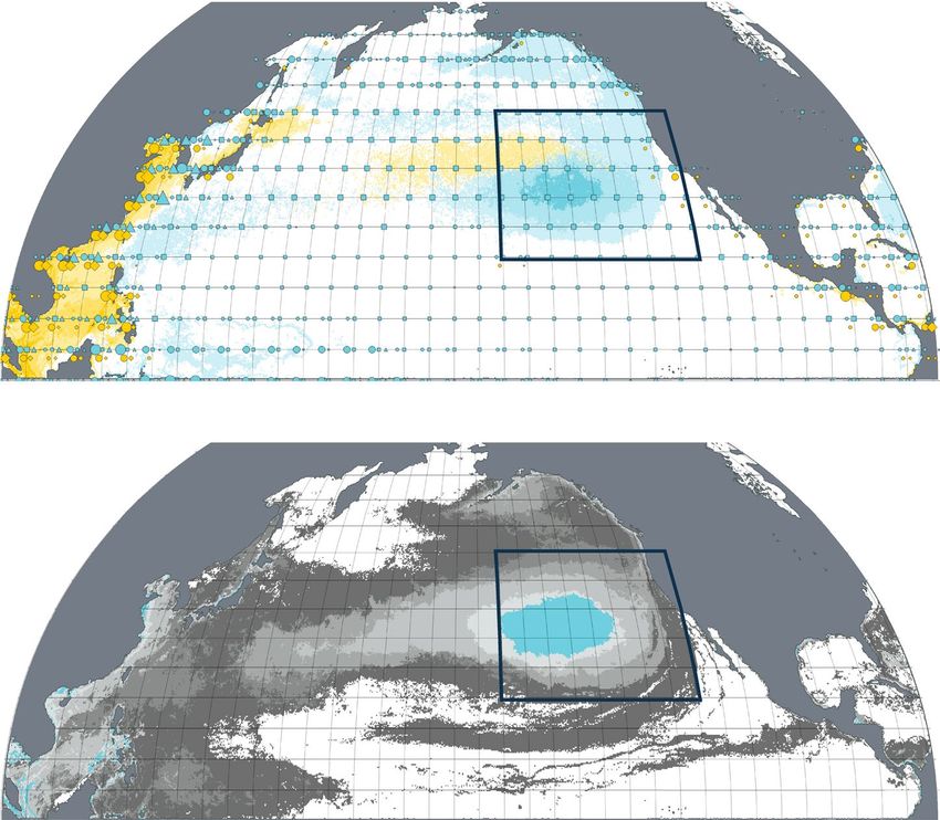
www.nature.com/scientificreports/

                              Figure 1. Field monitoring effort. Vessel (grey and dark blue lines) and aircraft (light blue lines) tracks and
                              locations where data on buoyant ocean plastic concentrations were collected (circles). Grey circles (n = 350)
                              represent areas sampled with a single Manta net tow by 17 participating vessels, between July and September
                              2015. Dark blue circles (n = 76) represent areas sampled with paired Manta and paired Mega net tows by RV
                              Ocean Starr, between July and August 2015. Light blue circles (n = 31) show locations of RGB geo-referenced
                              mosaics collected from a C-130 Hercules aircraft, in October 2016. This map was created using QGIS version
                              2.18.1 (www.qgis.org).

                              mostly attributed to a connection to substantial ocean plastic sources in Asia23,24 through the Kuroshio Extension
                              (KE) current system25 as well as intensified fishing activity in the Pacific Ocean26.
                                  Most available data on quantities and characteristics of buoyant ocean plastic are derived from samples col-
                              lected with small sea surface trawls initially developed to collect neustonic plankton27. Due to their small aperture
                              (0.5–1 m width, 0.15–1 m depth) and limited surface area covered, they could underestimate loads of rarer and
                              larger plastic objects such as bottles, buoys and fishing nets. In an attempt to overcome this misrepresentation, a
                              research team21 combined net tow data with information from vessel-based visual sighting surveys. They found
                              that while small, millimetre-sized pieces (50 cm plastic objects (Fig. 1).

ScienTific REPOrTS | (2018) 8:4666 | DOI:10.1038/s41598-018-22939-w                                                                              2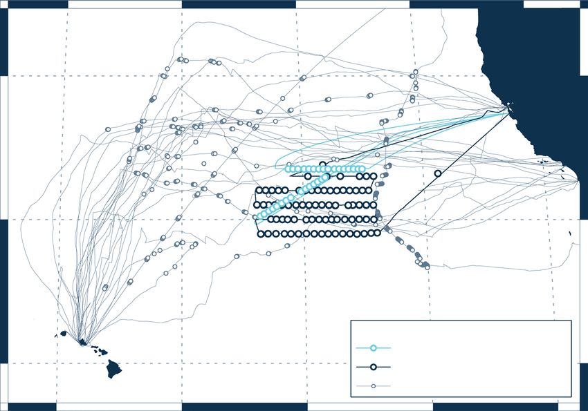
www.nature.com/scientificreports/

                                  Vessels carried out net tows of 0.35–4 hours duration, while navigating at 0.7–6.8 knots. All trawls were
                              designed to move away from the vessel to avoid wake effects on the capture efficiency of the devices. All vessel
                              crews were trained with online material and one-to-one workshops that had been conducted prior to departure.
                              While towing the trawl, the most experienced sailor aboard the vessel estimated the sea state (Beaufort scale) by
                              measuring wind speeds and observing wave heights. This data was recorded in the standard datasheets provided,
                              alongside the date, duration, as well as initial and final coordinates of each tow. The location and length of all
                              net tows were confirmed during the post-processing phase by inspecting the position data from GPS trackers
                              installed on all participating vessels. Most sampling stations encompassed a single net tow (n = 350 sampling
                              stations) using a Manta trawl (0.5 mm square mesh, 90 cm × 15 cm mouth), which is one of the standard devices
                              for quantifying plastic pollution levels. With the largest participating vessel (RV Ocean Starr), we simultaneously
                              towed two Manta trawls, alongside two large Neuston trawls (1.5 cm square mesh, 6 m × 1.5 m mouth, of which
                              0.5 m above the water line; thereafter called ‘Mega trawls’) at every sampling location (n = 76 stations). After each
                              Manta net tow, the net was rinsed from the outside with seawater, and its single-use cod-end removed, closed
                              with staples and placed in an individual zip-lock bag. After each Mega trawl tow, the net was also rinsed from
                              the outside with seawater and its large cod-end opened in a box filled with seawater. All buoyant plastics were
                              then removed, wrapped in aluminium and placed in labelled plastic bags. The whole content captured by the
                              Manta trawls was stored, while the organisms captured by the Mega trawls (mostly alive) were released back into
                              the ocean. All samples were stored in a fridge or freezer while at-sea, and in a FedEx cool box (2–8 °C) or reefer
                              (−2 °C) while being shipped to the laboratory. Even though we were careful when handling samples, some debris
                              items may have been broken during transportation, leading to some bias in our debris size distribution. Detailed
                              information related to these net tows (i.e. coordinates, metocean conditions, sampling times and durations) is
                              provided in Figshare33.
                                  The aerial surveys sampled a far greater area (311.0 km2) than the trawl surveys described above (3.9 km2 and
                              13.6 km2, for Manta and Mega net tows, respectively), thus yielding a more reliable quantification of debris larger
                              than 50 cm, which are relatively rare. Both flights started and ended at Moffett Airfield near Mountain View,
                              California. The first aerial survey was conducted on October 2nd 2016 sampling from 18:56 to 21:14 UTC time,
                              at a constant latitude of 33.5°N, and longitudes varying from 141.4°W to 134.9°W. The second survey started on
                              October 6th 2016 sampling from 22:14 to 0:37 UTC, from 30.1°N, 143.7°W to 32.9°N, 138.1°W. While in survey
                              mode, the aircraft flew at an altitude of approximately 400 m and at a ground speed of 140 knots. Sampling tran-
                              sects targeted areas where the sea state conditions were the lowest, based on the weather forecast, including sea
                              surface atmospheric pressure, cloud cover, wind speed at 10 m above sea level and boundary surface layer height
                              provided by NOAA’s Global Forecasting System, as well as significant wave height and peak period data distrib-
                              uted by NOAA’s WaveWatch3 model outputs. Even though we surveyed floating debris using trained observers
                              and three types of sensor (Lidar, SWIR imager, and RGB camera), here we only analyse information coming from
                              the geo-referenced mosaics produced by a RGB camera (CS-4800i) that generally took photographs every second
                              during surveying time (frame size = ~360 m across track, ~240 m along track, ~0.1 m resolution).

                              Trawl samples processing.                Trawl samples were separately washed into a sieve tower (five Glenammer
                              Engineering Ltd sieves, with 0.05 cm, 0.15 cm, 0.5 cm, 1.5 cm, and 5 cm square apertures) that divided the material
                              into the following size classes: 0.05–0.15 cm, 0.15–0.5 cm, 0.5–1.5 cm, 1.5–5 cm, and >5 cm. Debris items >5 cm
                              were then manually sorted into 5–10 cm, 10–50 cm, and >50 cm classes by measuring the object lengths (widest
                              dimension of the object) with a ruler. Buoyant debris was separated from biomass by placing the material within
                              each sieve in filtered saltwater (salinity 3.5%, temperature 19–23 °C). Lab personnel stirred the material many
                              times to insure floating particles were detached from the biomass material. Floating objects identified as buoyant
                              debris were manually extracted from the water surface using forceps, separated into types, and counted. Buoyant
                              debris was classified into material type (plastic, glass, paraffin, tar, rubber, wood, pumice, seed or unknown), with
                              plastics being further divided into the following categories: (1) ‘H’ type – fragments and objects made of hard
                              plastic, plastic sheet or film; (2) ‘N’ type – plastic lines, ropes, and fishing nets; (3) ‘P’ type – pre-production plastic
                              pellets in the shape of a cylinder, disk or sphere; and (4) ‘F’ type – fragments or objects made of foamed material
                              (e.g. expanded polystyrene). Once counted and categorized, the pieces were washed with distilled water, trans-
                              ferred to aluminium dishes, dried overnight at 60 °C, and weighed using an OHAUS Explorer EX324M (0.0001 g
                              readability) for objects 5 cm.
                                  To best characterize the ocean plastic accumulating within the GPGP, we performed additional analyses with
                              the material collected. Firstly, 10 pieces within each plastic size/type category (n = 220 pieces) were selected for
                              polymer composition analysis by Fourier-transform infrared spectroscopy (FT-IR). The readings were done using
                              a Perkin Elmer Spectrum 100 FT-IR equipped with a universal ATR accessory (range = 600–4000 cm−1). The
                              respective polymer type was determined by comparing sample FT-IR spectra against known spectra from a data-
                              base (Perkin-Elmer ATR of Polymers Library). Secondly, we screened all plastic debris collected for production
                              dates, as well as any writings statements giving information on its origin (i.e. language and ‘made in’ statements).
                              Lastly, we classified plastic items from ‘H’ and ‘L’ types collected at 30 RV Ocean Starr stations into object types
                              (e.g. bottle lids, bags, bottles, etc). As ‘H’ objects larger than 50 cm were relatively rare, we analysed 10 extra RV
                              Ocean Starr stations for this type/size category. If the object type of a fragment could not be determined, we clas-
                              sified the piece as either hard plastic fragment or film fragment depending on its wall thickness and flexibility34.
                              We used Manta trawl samples to characterise objects within size classes 0.15–0.5 cm, 0.5–1.5 cm, and 1.5–5 cm,
                              and Mega trawl samples to characterise objects within size classes 5–10 cm, 10–50 cm, and >50 cm. Plastics within
                              our smallest size class (0.05–0.15 cm) were not considered in this ‘Object Type’ analysis due to the difficulty of
                              handling and identifying small fragments.
                                  The numerical/mass concentrations of buoyant plastic items (count/kg of plastic per km2 of sea surface) meas-
                              ured by each net tow were calculated for all plastic size/type categories separately. To do so, we divided the count

ScienTific REPOrTS | (2018) 8:4666 | DOI:10.1038/s41598-018-22939-w                                                                                     3
www.nature.com/scientificreports/
and weight of plastic objects within each category by the towed area of the sample. We calculated the towed area
by multiplying net mouth width (90 cm for Manta trawl, 6 m for Mega trawl) by tow length (determined from
GPS position data). The average area covered by Manta net tows was 0.008 km2 (SD = 0.004, min–max: 0.001–
0.018 km2), while the average area covered by Mega net tows was 0.090 km2, (SD = 0.013, min–max: 0.046–0.125
km2). As buoyant plastics can be missed by surface trawls due to wind-driven mixing, we then estimated the
‘depth-integrated’ mass and numerical plastic concentrations (Ci) for all type/size categories at each of the trawl
sampling locations using the equations described in ref.35. Supplementary Methods 1 provides details on how Ci
was calculated as a function of ocean plastic terminal rising velocity (Wb), depth sampled by the trawl, and sea
state. It also describes how we measured Wb for each of the type/size categories of this study. After comparing
plastic concentration results obtained by paired Manta and Mega net tows (n = 76 locations), we decided to use
Manta and Mega trawl samples to quantify debris 0.05–5 cm and 5–50 cm in size, respectively. The comparison
results and reasoning behind such decision in provided in Supplementary Methods 2.
Aerial imagery processing. All RGB images taken during our survey flights (n = 7,298) were georefer-
enced using accurate aircraft position and altitude data collected during the surveys. They were then inspected
by two trained observers and a detection algorithm. Observers inspected all images at full-screen on a Samsung
HD monitor (LU28E590DS/XY) and those single-frame mosaics containing debris were uploaded into QGIS
software (Version 2.18.3–Las Palmas) to record their position and characteristics. We trust we had a very small
number of false positives and a high number of false negatives. This is because the observers took a conservative
approach: they only logged features as debris when they were very confident with its identification. As such, many
features that could be debris, but resembled other natural features, such as sun glint and breaking wave, were not
logged into our ocean plastic dataset. Once this work was finalised, we ran an experimental algorithm capable
of detecting potential debris in all our RGB mosaics as a quality control step. To avoid any false positives, all fea-
tures detected by the algorithm were also visually inspected by an observer and only those visually identified as
debris were logged in our QGIS database. For every sighting, we recorded position (latitude, longitude), length
(widest dimension of the object), width, and object type: (1) ‘bundled net’ – a group of fishing nets bundled
tightly together; they are commonly colourful and of a rounded shape; (2) ‘loose net’ – a single fishing net; they
were generally quite translucent and rectangular in shape; (3) ‘container’ – rectangular and bright objects, such as
fishing crates and drums; (4) ‘rope’ – long cylindrical objects around 15 cm thick; (5) ‘buoy/lid’, rounded bright
objects that could be either a large lid or a buoy; (6) ‘unknown’ – objects that are clearly debris but whose object
type was not identified, they were mostly irregular-shaped items resembling plastic fragments; and (7) Other
– only one object was successfully identified but did not belong to any category above: a life ring. We recorded
1,595 debris items (403 and 1,192 in flights 1 and 2 respectively); 626 were 10–50 cm and 969 were >50 cm in
length. Most of them were classified as ‘unknown’ (78% for 10–50 cm, 32% for >50 cm), followed by ‘buoy or lid’
(20%) and ‘bundled net’ (1%) for 10–50 cm debris, and by ‘bundled net’ (29%), ‘container’ (18%), ‘buoy or lid’
(9%), ‘rope’ (6%), and ‘lose net’ (4%) for >50 cm debris. To calculate ocean plastic concentrations, we grouped the
geo-referenced images into 31 ~10 km2 mosaics. For numerical concentrations, we simply divided the number
of debris pieces 10–50 cm and >50 cm within each mosaic by the area covered. To estimate mass concentrations,
we had to first estimate the mass of each object spotted, then we separately summed the mass of 10–50 cm and
>50 cm debris within each mosaic by the area covered. More information on how we estimated the mass of each
spotted objects is provided in Supplementary Methods 3.
Numerical model formulation. Ocean plastic pathways can be represented by Lagrangian particle trajec-
tories31. In our framework, particles were advected by the following environmental drivers: sea surface currents,
wave induced Stokes drift and winds. Starting from identical particle releases, we produced a series of forcing
scenarios to represent the diversity in shape and composition of ocean plastics. Starting from using sea surface
current only, we gradually added forcing terms representing the actions of atmospheric drag and wind waves
on buoyant debris. The action of wind was simulated by considering the displacement of particles as a fraction
of wind speed at 10 m above sea level. This is referred as the ‘windage coefficient’. We assessed different windage
coefficient scenarios including 0%, 0.1%, 0.5%, 1%, 2% and 3%. We sourced global sea surface currents (1993
to 2012) from the HYCOM + NCODA global 1/12° reanalysis (experiment 19.0 and 19.136–38), and wind (10 m
above sea level) speed and direction data (1993 to 2012) from NCEP/NCAR global reanalysis39. Wave induced
Stokes drift amplitude was calculated using wave spectrum bulk coefficients (significant wave height, peak wave
period and direction) from Wavewatch3 model outputs40.
For every forcing scenario, particles were identically and continuously released in time from 1993 to 2012
following spatial distributions and amplitudes of significant ocean plastic sources on land (coastal population
hotspots23 and major rivers24) as well as at sea (fishing26,41, aquaculture42 and shipping industries43). Source
scenarios were combined using relative source contribution as well as geographical distribution presented in
Supplementary Methods 4. We advected global particles in time using the forcing scenarios described above and
successfully reproduced the formation of oceanic garbage patches, with the shape and gradient of particle concen-
trations in these areas differing amongst forcing scenarios. We computed daily particle visits over 0.2° resolution
grids corresponding to our observation domain and extending from 160°W to 120°W in longitude and 20°N to
45°N in latitude. The number of daily particle visits was uniformized over the total number of particles present in
the global model at a given time. The model-predicted non-dimensional concentration δi of cell i, was calculated
as follows:
δi = ∑αs δi ,s
s (1)
ScienTific REPOrTS | (2018) 8:4666 | DOI:10.1038/s41598-018-22939-w 4www.nature.com/scientificreports/
where αs is the non-dimensional weight relative to the contribution of source s and δi,s is the percentage of global
particles from source s in cell i. δi,s is calculated with the number of particles ni,s from source s in cell i over the
total number of global particles Σins from source s:
ni , s
δi , s =
∑ i ns (2)
Numerical model calibration. We collected measurements at sea in 2015 and 2016, but our numerical
model uses ocean circulation reanalysis covering the period from 1993 to 2012. Modelled ocean circulation data
post-2012 is available from HYCOM however not as a reanalysis product. As such, we decided not to use it in
this study. As initial model particles released in 1993 significantly start to accumulate in the area after about 7
years, we averaged uniformized daily particle visits over 12 years, from 2000 to 2012. We grouped observed debris
size classes in four categories: microplastics (0.05–0.5 cm), mesoplastics (0.5–5 cm), macroplastics (5–50 cm)
and megaplastics (>50 cm). We compared model predictions against depth-integrated microplastic concen-
trations as this dataset collected by Manta trawls had the largest spatial coverage. Mass concentrations derived
from trawl measurements were grouped in 0.2-degree resolution cells and compared against model-predicted
non-dimensional concentration δ for the five different forcing scenarios. The best model fit was found for the
forcing scenario with sea-surface current only (R2 = 0.52, n = 277 cells). The regression coefficient declined as we
increased the atmospheric drag term (R2 = 0.39 to 0.21 depending on windage coefficient).
As we analysed the accumulation of model particles in the GPGP region, we noticed significant seasonal and
inter-annual variations of the GPGP position. The modelled GPGP dimensions was relatively consistent through-
out our 12 years of analysis, but the relative position of this accumulation zone varied with years and seasons. We
first decided to test our model for seasonal variation by comparing our microplastic concentrations (measured in
July – September 2015) against modelled concentrations averages for the July–September periods of 2000 to 2012.
This comparison yielded poorer results (R2 = 0.46 to 0.21, depending on forcing scenario) than with the 12 years
average solution (R2 = 0.52) as the July–September GPGP position varied substantially among years.
The relation between the accumulation of marine debris in the North Pacific and climate events such as El
Niño Southern Oscillation (ENSO) and the Pacific Decadal Oscillation (PDO) has previously been discussed18.
As such, to account for inter-annual variation, we compared latitudinal and longitudinal position of the GPGP
against these two climate indexes: ENSO and PDO. We found that 2002 and 2004 were similar to the conditions
experienced during our multi-vessel expedition. Thus, we compared our measurements against particle visit aver-
ages for July–September of 2002 and 2004 combined. This second attempt exhibited better results (R2 = 0.58 to
0.41, depending on forcing scenario), suggesting that climatic events such as ENSO or PDO influence the aver-
age position of the GPGP. Therefore, we decided to use the July–September average for 2002 and 2004, which
better accounts for inter-annual variations in the GPGP position. More information on the selection of years for
calibrating the model against trawl and aerial surveys data is provided in Supplementary Methods 5. The best fit
between model predictions and microplastic observations was found once again for the forcing scenario with sea
surface current only (R2 = 0.58, n = 277). The best regression fit between measured and modelled microplastic
concentrations had a = −8.3068 and b = 0.6770 in the parametric formulation:
log 10δ− a
cmod = 10 b (3)
From this formulation, we computed the modelled microplastics mass concentration in our domain area and
extracted contour levels by order of magnitude, from 0.01 g km−2 to 10 kg km−2. The GPGP as defined in this
study corresponds to the 1 kg km−2 microplastic mass concentration level covering an area of 1.6 million km2
and depicted as a bold line in Fig. 2a. As a validation, we categorized microplastics measurements inside and
outside the 1 kg km−2 contour line (Fig. 2b). For stations inside the model-predicted GPGP, the median measured
microplastic concentration was 1.8 kg km−2 (25th–75th percentiles = 3.5–0.9 kg km−2) while for stations outside,
the median was 0.3 kg km−2 (25th–75th percentiles = 0.2–0.7 kg km−2). Using our calibrated microplastics distri-
bution, we computed the mass and numerical concentration for individual size classes from scaling modelled
concentrations by the ratio between average modelled microplastics distribution inside the GPGP and averaged
measured concentrations per size class of stations inside the patch. A comparison between measured and mod-
elled mass/numerical concentrations for all ocean plastic size classes is given in Fig. 2c and d.
Our confidence intervals were formulated to account for uncertainties in both sampling and modelling.
For the trawl collection (i.e. micro-, meso- and macroplastics), we considered uncertainties related to the
vertical-mixing corrections applied to surface concentrations using reported sea state and plastic’s rising veloci-
ties (see Supplementary Methods 1). For the aerial mosaics, we accounted for uncertainties related to estimating
the mass of sighted objects based on correlations between top-view area and dry weight of objects collected in the
trawls (see Supplementary Methods 3). Finally, to account for modelling uncertainties, we added (respectively
subtracted) the standard error of measured concentration to (resp. from) the mean upper (resp. lower) mass con-
centration when scaling the microplastics distribution to individual size classes.
Characterisation by types, sources and forcing scenarios. The total estimated mass load of ocean
plastic in the GPGP by size classes were further divided by types. We calculated the average fraction in mass
of individual ocean plastic types per sampling event for stations inside the patch (Supplementary Table 1) and
derived the contribution of types ‘H’, ‘N’, ‘F’ and ‘P’. Further, as we predominantly observed debris originated
from marine sources, we investigated the source contribution predicted by our calibrated modelled distribution.
For individual model cells, we calculated the percentage of Lagrangian particle visits from individual sources.
ScienTific REPOrTS | (2018) 8:4666 | DOI:10.1038/s41598-018-22939-w 5www.nature.com/scientificreports/
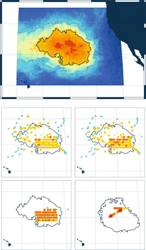
Figure 2. Numerical model calibration. (a) The GPGP boundary (blue line) is estimated by comparing
microplastic concentration measurements (circles) to model particle visit averages that accounted for seasonal
and inter-annual variations. This map was created using QGIS version 2.18.1 (www.qgis.org). (b) Model
validation showing median measured mass concentration for microplastics of stations outside and inside
our predicted 1 kg km−2 GPGP boundary. Bars extend from 25th to 75th percentile while whiskers extend to
minimum and maximum non-outlier. Outliers are represented as crosses. (c) Measured mass concentrations
versus modelled mass concentrations for microplastics, mesoplastics, macroplastics and megaplastics. (d) Same
as (c) but with numerical concentrations.
As initial particles were weighted in accordance to estimated global inputs, model particles from marine sources
originally represented 28.1% of the total amount of material with fishing (17.9%), aquaculture (1.3%) and ship-
ping (8.9%). We calculated the difference from this initial percentage value for each model cell and reported it to
the predicted total mass concentration. In doing so, we defined ‘anomalies’ in marine source contribution in the
North Pacific and expressed these in unit of mass per surface area. Finally, even though our calibrated model con-
sidered sea surface current only, we compared the predominance of forcing scenarios by evaluating the respective
number of particle visits for each model cells. We computed contours around the GPGP for individual forcing
scenarios in a way that the material contained inside each contour is equal to our initial forcing scenario (i.e. sea
surface current only).
The dependence of the particle trajectory on the windage coefficient predicted by our model is in good agree-
ment with sightings and modelling of debris originated from the 2011 Tohoku tsunami in Japan44,45. The first
identified Japanese debris items that arrived after 10 to 12 months on the North American shores were objects
with high windage such as buoys, boats and floating docks. Debris also arrived on Hawaiian Islands 18 months
after the incident. The time of arrival was closely related to object types, starting in the first year with large oyster
farm buoys and other floats, containers, and canisters. In the second year more buoys, tipped boats, fridges, and
pallets arrived, followed later by timber beams and wooden debris. Our model predicted that only objects with
a windage coefficient above 3% could arrive on Hawaii in the second year after the 2011 tsunami. Objects with
ScienTific REPOrTS | (2018) 8:4666 | DOI:10.1038/s41598-018-22939-w 6www.nature.com/scientificreports/
windage coefficient ranging from 1 to 2% would reach Hawaii during the third year, while objects with no wind-
age would mostly accumulate in the GPGP, north east of the archipelago.
Long term analysis. The definition of a dynamic GPGP boundary that accounts for seasonal and
inter-annual variabilities allowed us to estimate which sea surface trawl data points from the literature are
inside or outside the GPGP region. Therefore, we used our calibrated model to assess the decadal evolution of
microplastic mass concentrations (kg km−2) within and around the GPGP. Concentration data from the literature
(Supplementary Table 2) was obtained from published datasets or digitized from figures when not available digi-
tally17,46,47. When data was reported in unit of mass per volume of water48, we used the net tow depth to calculate
the concentration per surface area unit. When only numerical concentration was reported22,48, we estimated mass
concentration by using the average ocean plastic mass from net tows where both mass and numerical concentra-
tions were reported (m = 3.53 mg, SE: 0.10 mg, n = 872).
We compared the model-predicted GPGP boundary with the locations of samples collected between 1999 and
201221,22,48,49. Samples collected before 199917,46–48 were compared against the GPGP position estimated for the
sampled months and years in the 1999–2012 period that had similar ENSO and PDO values (See Supplementary
Methods 6). Using our dynamic GPGP model boundary as reference, we classified each net tow into 3 categories:
(1) sampled within the GPGP boundary, (2) sampled outside the GPGP boundary, but above 20°N and below
45°N and (3) sampled in the rest of the North Pacific. We only used net tows from the first two categories above
so that concentration statistics for outside the patch were not biased by measurements taken in equatorial and
polar waters, where concentrations were very low. We then grouped these microplastic concentration observa-
tions from plankton net trawls by decades, taking data recorded between 1965–1974 (n = 20 inside and n = 58
outside17,48), 1975–1984 (n = 0 inside and n = 19 outside46), 1985–1994 (n = 4 inside and n = 2 outside47), 1995–
2004 (n = 2 inside and n = 252 outside22,49), 2005–2014 (n = 195 inside and n = 861 outside21,22,48) and finally
2015 (n = 288 inside and n = 213 outside; this study). We calculated the mean (± standard error) of measured
microplastic mass concentration per decades for within and around the GPGP boundary. Finally, we extracted
decadal trends by fitting an exponential function (R2 = 0.94) assuming null concentrations at the beginning of
the 20th century. The exponential fit exhibited better results than linear, quadratic or cubic functions (R2 = 0.71,
R2 = 0.86 and R2 = 0.91, respectively).
Results
Ocean plastic loads and characteristics. Plastics were by far the most dominant type of marine litter
found, representing more than 99.9% of the 1,136,145 pieces and 668 kg of floating debris collected by our trawls.
We estimated that an area of 1.6 million km2 holds ocean plastic concentrations ranging from 10 s to 100 s kg
km−2 (Fig. 3). This area, which comprises ~87% of the ocean plastic material present in our model domain
(120°W–160°W, 20°N–45°N), defines the Great Pacific Garbage Patch (GPGP) boundary for this study. We
predicted that the GPGP contains a total of 1.8 (mid-point estimate, low: 1.1, high: 3.6) trillion plastic pieces
weighing 79 k (45 k−129 k) tonnes, comprised of debris categorised in 4 size classes: microplastics (0.05–0.5 cm),
mesoplastics (0.5–5 cm), macroplastics (5–50 cm), and megaplastics (>50 cm). Out of this total, we estimated
1.7 (1.1–3.5) trillion pieces and 6.4 k (4.1 k–12 k) tonnes of microplastics, 56 (39–104) billion pieces and 10 k
(6.9 k–19 k) tonnes of mesoplastics, 821 (754–908) million pieces and 20k (18 k–22 k) tonnes of macroplastics,
and 3.2 (2.7–3.6) million pieces and 42 k (16 k–75 k) tonnes of megaplastics (Table 1).
More than three quarters of the GPGP plastic mass was contained in the upper size classes (>5 cm), with a
respective total contribution of 25% and 53% for macroplastics and megaplastics (Fig. 4a). Plastic types ‘H’ (hard
plastics, sheets and films) and ‘N’ (nets, ropes and lines) represented respectively 47% and 52% of the total GPGP
plastic mass, with most of micro-, meso- and macroplastic mass coming from type ‘H’, and megaplastic from type
‘N’. Two additional plastic types, pellets (type ‘P’) and foams (type ‘F’) were also observed in a few size classes,
but their overall contribution to the GPGP plastic load was minimal. For megaplastics, we could also assess the
mass contributions of different object types. We estimated that 86% of their 42 k tonnes contribution was carried
by fishing nets.
Megaplastics generally yielded the highest observed mass concentration with mean measured values of
46.3 kg km−2 (min–max: 0.4–428.1 kg km−2), followed by macroplastics with 16.8 kg km−2 (0.4–70.4 kg km−2),
mesoplastics with 3.9 kg km−2 (0.0003–88.4 kg km−2), and microplastics with 2.5 kg km−2 (0.07–26.4 kg km−2).
Regarding abundance however, microplastics and mesoplastics were by far the most numerous, with mean meas-
ured concentrations of 678,000 (min–max: 20,108–11,054,595) and 22,000 (261–321,712) pieces km−2 inside the
GPGP against 690 (40–2,433) and 3.5 (0.5–11.6) pieces km−2 for macroplastics and megaplastics, respectively
(Fig. 4b, Table 2).
The polymer composition of ocean plastic collected in the GPGP were analysed by Fourier-transform infra-
red spectroscopy. Polyethylene (PE) and polypropylene (PP) were by far the most common polymer types
(Supplementary Table 3). Object type was rarely identifiable as most particles consisted of fragments. Plastic
objects that could be identified (either entire or in early stages of fragmentation) included containers, bottles, lids,
bottle caps, packaging straps, eel trap cones, oyster spacers, ropes, and fishing nets (Supplementary Table 4). Age
and geographical origin evidences were found on some objects, with 50 items having a readable production date:
1 in 1977, 7 in the 1980s, 17 in the 1990s, 24 in the 2000s and 1 from 2010. We also found 386 objects with recog-
nizable words or sentences written in 9 different languages. One third had Japanese inscriptions (115 objects) and
another third had Chinese (113 objects). The rest was divided among nine countries (Supplementary Table 5)
Furthermore, a country of production was identified on 41 objects (‘made in’ label), manufactured in 12 different
countries (see Supplementary Table 5).
ScienTific REPOrTS | (2018) 8:4666 | DOI:10.1038/s41598-018-22939-w 7www.nature.com/scientificreports/
Figure 3. Modelled and measured mass concentration in the Great Pacific Garbage Patch (GPGP). (a) Ocean
plastic mass concentrations for August 2015, as predicted by our data-calibrated model. The bold black line
represents our established limit for the GPGP. (b) Microplastics (0.05–0.5 cm) mass concentrations as measured
by Manta trawl (n = 501 net tows, 3.8 km2 surveyed). (c) Mesoplastics (0.5–5 cm) mass concentrations as
measured by Manta trawl; d) Macroplastics (5–50 cm) mass concentrations as measured by Mega trawl
(n = 151 net tows, 13.6 km2 surveyed); (e) Megaplastics (>50 cm) mass concentrations as estimated from aerial
imagery (n = 31 mosaic segments, 311.0 km2 surveyed). All observational maps are showing mid-point mass
concentration estimates as well as the predicted GPGP boundaries for the corresponding sampling period:
August 2015 for net tow samples, and October 2016 for aerial mosaics. Maps were created using QGIS version
2.18.1 (www.qgis.org).
ScienTific REPOrTS | (2018) 8:4666 | DOI:10.1038/s41598-018-22939-w 8www.nature.com/scientificreports/
Size Class
(cm) Type H Type N Type P Type F All
581 23 604
(tonnes) — 0.2 (0.1–0.4)
(351–1,252) (14–49) (365–1,302)
0.05–0.15
1.0 1012
6.4 1010
4.5 108 1.1 1012
(#) —
(6.3 1011–2.2 1012) (3.9 1010–1.4 1011) (2.7 108–9.5 108) (6.7 1011–2.3 1012)
5,356 82 336 1.8 5,776
(tonnes)
(3,498–10,035) (54–154) (219–630) (1.2–3.4) (3,772–10,821)
0.15–0.5
5.6 1011 4.9 1010 2.2 1010 5.4 108 6.3 1011
(#)
(3.6 1011–1.0 1012) (3.2 1010–9.0 1010) (1.5 1010–4.1 1010) (3.5 108–9.9 108) (4.1 1011–1.2 1012)
4,703 159 0.9 4,865
(tonnes) 3 (2–5)
(3,255–8,590) (110–290) (0.6–1.6) (3,367–8,886)
0.5–1.5
4.2 1010 9.5 109 2.7 107 3.9 107 5.1 1010
(#)
(2.9 1010–7.8 1010) (6.6 109–1.8 1010) (1.9 107–5.0 107) (2.7 107–7.3 107) (3.6 1010–9.6 1010)
4,662 439 5,106
(tonnes) — 5 (4–11)
(3,220–9,642) (303–907) (3,527–10,560)
1.5–5
2.8 109 1.5 109 1.5 107 4.36 109
(#) —
(2.0 109–5.4 109) (1.1 109–2.8 109) (1.1 107–2.9 107) (3.2 109–8.3 109)
1,899 120 0.8 2,020
(tonnes) —
(1,714–2,166) (108–137) (0.7–0.9) (1,823–2,304)
5–10
2.1 108 6.5 107 4.7 105 2.7 108
(#) —
(1.9 108–2.3 108) (6.0 107–7.3 107) (4.3 105–5.3 105) (2.5 108–3.1 108)
16,742 1,409 18,175
(tonnes) — 24 (22–27)
(15,265–18,330) (1,284–1,542) (16,572–19,899)
10–50
3.4 108 2.1 108 9.0 105 5.5 108
(#) —
(3.1 108–3.7 108) (1.9 108–2.3 108) (8.2 105–9.8 105) (5.0 108–6.0 108)
3,217 39,144 42,362
(tonnes) — —
(1,195–5,688) (14,540–69,203) (15,736–74,892)
>50
1.9 106 1.3 106 3.2 106
(#) — —
(1.6 106–2.2 106) (1.1 106–1.5 106) (2.7 106–3.6 106)
37,162 41,376 337 35 78,909
(tonnes)
(28,500–55,704) (16,414–72,283) (220–631) (29–46) (45,163–128,665)
All
1.6 1012 1.2 1011 2.2 1010 1.1 109 1.8 1012
(#)
(1.0 1012–3.3 1012) (7.9 1010–2.5 1011) (1.5 1010–4.1 1010) (6.7 108–2.1 109) (1.1 1012–3.6 1012)
Table 1. Mass and numerical load per ocean plastic type and size within the 1.6 million km2 GPGP. Plastic type
H include pieces of hard plastic, plastic sheet and film, type N encompasses plastic lines, ropes and fishing nets,
type P are pre-production plastic pellets, and type F are pieces made of foamed material.
Source, formation and temporal evolution predictions. Our global model simulated the release of
Lagrangian particles from significant sources of ocean plastic. It predicted that the relative contribution of marine
sources (fishing, shipping and aquaculture industries) to the GPGP plastic load was above global average (Fig. 5a).
Model particles were transported under a series of environmental forcing scenarios representing sea surface
current (0–10 m), wave-induced Stokes drift, and 0.1%, 0.5%, 1%, 2% and 3% of wind velocities at 10 m above
sea surface. The best model representation (R2 = 0.58, n = 277) was established with a windage coefficient of
0%, as this scenario best reproduced the several orders of magnitude differences between concentrations within
and around the GPGP region. When considering particles from all forcing scenarios investigated in this study
(Fig. 5b), our model predicted that the GPGP is dominated by sea surface current-driven particles, with wind
influence increasing as the orbits around the patch become wider. Particles subject to greater atmospheric drag
were more likely to escape the GPGP, circling around the North Pacific subtropical gyre if exiting from the south
or, entering the North Pacific subpolar gyre near Alaska if leaving from the north. We also noticed that the higher
the windage coefficient, the more likely a particle was to encounter landmass.
Our model resolved the temporal variability of ocean plastic accumulation in the ocean. This allowed us to
predict where the GPGP is located at monthly intervals. The GPGP position showed clear inter-annual variations,
with latitudinal position of its centre oscillating around 32°N and some frequent temporary displacement south-
ward (26°N to 30°N depending on the forcing scenario). It also demonstrated a clear seasonal variation in the
longitudinal position, with its predicted centre oscillating around 145°W and appearing to shift from west to east
between boreal winter and summer. Both GPGP latitudinal and longitudinal oscillations intensified with higher
atmospheric drag term components. The centre latitude and longitude showed a statistically significant correla-
tion with respectively, the El Niño Southern Oscillation (ENSO50; R = 0.26, p = 0.0011, n = 156) and the Pacific
Decadal Oscillation (PDO51, R = 0.71, p < 0.001, n = 156) indexes. A dynamic GPGP model boundary allowed us
to determine whether surface net tows from previous studies17,21,22,46–49 were sampling inside or outside the GPGP.
Average plastic mass concentration measured by net tows inside the GPGP boundary showed an exponential
increase over the last decades, rising from an average 0.4 (±0.2 SE, n = 20) kg km−2 in the 1970s to 1.23 (±0.06
SE, n = 288) kg km−2 in 2015 (Fig. 6). Historical samples collected at subtropical latitudes (20°N−45°N) around
the GPGP also showed an exponential increase during the same time period but at a slower rate than inside the
accumulation zone.
ScienTific REPOrTS | (2018) 8:4666 | DOI:10.1038/s41598-018-22939-w 9www.nature.com/scientificreports/
Figure 4. Ocean plastic size spectrum in the GPGP. (a) Plastic mass distribution within the GPGP between
size (bars) and type (colours) classes. Plastic type H include pieces of hard plastic, plastic sheet and film, type
N encompasses plastic lines, ropes and fishing nets, type P are pre-production plastic pellets, and type F are
pieces made of foamed plastics. Whiskers extend from lower to upper estimates per size class, accounting for
uncertainties in both monitoring and modelling methods. (b) Measured mass and numerical concentrations of
GPGP ocean plastics. Dots represent the mean concentrations, the whiskers and darker shades represent our
confidence intervals, and the lighter shades extend from the 5th and 95th percentile of measured concentrations.
Mean mass concentration Mean numerical
Size class Type (kg km−2) concentration (# km−2)
H 2.33 643,930
N 0.041 19,873
Microplastic (0.05–0.5 cm)
P 0.13 14,362
F 0.001 216
H 3.68 20,993
N 0.23 803
Mesoplastic (0.5–5 cm)
P 0.0003 3.6
F 0.003 12
H 15.53 640
Macroplastic (5–50 cm) N 1.27 49
F 0.021 0.7
H 3.52 0.3
Megaplastic (>50 cm)
N 42.82 3.3
All All 69.58 700,886
Table 2. Mean observed mass and numerical concentrations within the 1.6 million km2 GPGP for different
size and type of ocean plastics. Plastic type H include pieces of hard plastic, plastic sheet and film, type N
encompasses plastic lines, ropes and fishing nets, type P are pre-production plastic pellets, and type F are pieces
made of foamed material.
Discussion
This study provides a detailed quantification and characterization of ocean plastic within a major oceanic plastic
pollution hotspot: the GPGP. The sea surface environment of this oceanic region is now dominated by polyeth-
ylene (PE) and polypropylene (PP) pieces, substantially outweighing other artificial and natural floating debris.
Our aerial survey data, combined with in-situ observations from two different trawl devices, supported the devel-
opment of a comprehensive assessment of all GPGP debris larger than 0.05 cm. Our model estimates that this
1.6 million km2 accumulation zone is currently holding around 42k metric tons of megaplastics (e.g. fishing
nets, which represented more than 46% of the GPGP load), ~20k metric tons of macroplastics (e.g. crates, eel
trap cones, bottles), ~10 k metric tons of mesoplastics (e.g. bottle caps, oyster spacers), and ~6.4 k metric tons of
microplastics (e.g. fragments of rigid plastic objects, ropes and fishing nets).
Our plastic mass estimate for the GPGP (~79 k tonnes) was nearly sixteen times higher than a previous study
(~4.8 k tonnes) that used net trawl data only29 and four times higher than another assessment (~21 k tonnes)
that combined net trawl data with vessel-based visual surveys21. We suggest that the increase in the estimate is
mainly explained by the use of more robust methods for quantifying macro- and megaplastics over larger sea
surface areas. For instance, aerial imagery allowed us to more accurately count and measure the size of sighted
objects, which undeniably reduced uncertainties in mass estimates when compared to vessel-based visual surveys.
Nonetheless, differences between estimates could also be attributed to increasing levels of ocean plastic pollution
ScienTific REPOrTS | (2018) 8:4666 | DOI:10.1038/s41598-018-22939-w 10www.nature.com/scientificreports/
Figure 5. Modelled source and forcing distributions. (a) North Pacific distribution of the ocean plastics sources
used in this study (blue and orange squares, circles and triangles), and predicted marine source (shipping,
fishing and aquaculture) anomalies in relation to the initial distribution of both marine- and land-based sources
(coastal urban centres and rivers). (b) Predicted North Pacific distribution of dominant forcing scenario.
Windage coefficient values correspond to the percentage contributions of wind forcing at 10 m above sea level.
Maps were created using QGIS version 2.18.1 (www.qgis.org).
Figure 6. Decadal evolution of microplastic concentration in the GPGP. Mean (circles) and standard error
(whiskers) of microplastic mass concentrations measured by surface net tows conducted in different decades,
within (light blue) and around (dark grey) the GPGP. Dashed lines are exponential fits to the averages expressed
in g km−2: f(x) = exp(a*x) + b, with x expressed in number of years after 1900, a = 0.06121, b = 151.3, R2 = 0.92
for within GPGP and a = 0.04903, b = −7.138, R2 = 0.78 for around the GPGP.
ScienTific REPOrTS | (2018) 8:4666 | DOI:10.1038/s41598-018-22939-w 11www.nature.com/scientificreports/
in the area, and particularly plastic inputs from the 2011 Tohoku tsunami. An estimated 4.5 million tonnes of
debris were washed at sea instantly, of which 70% may have sunk rapidly according to Japanese Government45.
This leaves 1.4 million tonnes of debris that could have been transported at the sea surface over longer distances44.
The potential tsunami debris contribution to the GPGP is supported by the origin evidences observed on some of
the objects collected: Japan was the main production country (34%) of collected plastic objects that had a ‘made
in’ label and Japanese was the most common language identified on the objects writings (30%), closely followed
by Chinese (29.8%). Considering our estimated global inputs of plastics into the ocean (5.32–19.3 million tonnes
y−1, see Supplementary Table 6), and assuming tsunami debris have the same fraction of low windage objects than
for global sources, our dispersal model suggests the contribution of the 2011 Tohoku tsunami would be around
10–20% of the debris input into the GPGP post 2011.
Despite an increase in the GPGP mass estimate, a great discrepancy between predicted and observed ocean
plastic concentrations remains. Considering currently accepted plastic inputs from land- and marine-based
sources, our global model predicted millions of tonnes of ocean plastic to be within the GPGP region, while we
only found tens of thousands of tonnes. This two-orders of magnitude difference suggests the existence of mecha-
nisms removing most of the plastic mass from the sea surface16 and/or fragmenting the plastic into pieces smaller
than those quantified here (www.nature.com/scientificreports/
our aerial mosaics are conservative as some plastics are likely to have been missed by our observers and detection
algorithm, or not considered as we only logged features that were clearly recognised as floating plastics.
Historical data from surface net tows (1970–2015) indicate that plastic pollution levels are increasing expo-
nentially inside the GPGP, and at a faster rate than in surrounding waters. While this does not necessarily mean
that the GPGP is the final resting place for ocean plastic reaching this region, it provides evidence that the plastic
mass inflow is greater than the outflow. The degradation rate of synthetic polymers in the marine environment
is poorly understood64, but it is known to depend on local environmental conditions, polymer types, shape and
coating of objects10. The relatively high occurrence of macroplastics with production dates from the 70 s, 80 s, and
90 s compared to more recent debris suggest that specific types of plastic (i.e. with high volume-to-surface ratios
and low windage) persist and accumulate in the GPGP region65. The mass of plastics floating in the GPGP was
mostly distributed in macro- and megaplastics. It is difficult to estimate how long it will take for all the material
currently present in the area to degrade in smaller pieces and eventually escape sea surface waters. Based on our
modelling results, it seems the bulk mass of material currently present in the GPGP is very unlikely to leave the
area and may slowly degrade into increasingly smaller pieces that can eventually either sink to the seafloor14, or
behave as water tracer due to its microscopic size and low Reynolds number66.
Our study provides a comprehensive assessment of the GPGP buoyant plastic loads and characteristics.
Nonetheless, a quantification of plastic inputs and outputs into and from the GPGP is required to better assess the
residence time of the plastics accumulating in this area. More research effort is needed to quantify ocean plastic
sources, transport and loss processes and subsequently implement them in ocean plastic transport models. For
instance, no study has recently estimated the global input of fishing gear losses at sea. Furthermore, coastal trans-
port of plastics and its interaction with coastlines worldwide is poorly understood and needs to be implemented
in current global models. Levels of plastic pollution in deep water layers and seafloor below the GPGP remain
unknown, and could be quantified through sampling. We encourage more sampling throughout the world’s
oceans, as well as the systematic monitoring of the GPGP as it is one of the few marine regions with a relatively
good historical dataset that allows us to understand long-term trends in oceanic plastic pollution. We also sug-
gest focussing research efforts towards the development of more cost-effective monitoring methods, with better
spatio-temporal coverage67 and/or capacity to track ocean plastic movements68. Air- and space-borne remote
sensing technologies may drastically increase our knowledge of ocean plastic transport and certainly represent a
great prospect for the future of the ocean plastic research field. Recent advances in commercial satellite imagery
for instance may already allow us to identify meter-sized debris items, such as large ghostnets, which are a major
contributor to oceanic plastic pollution levels and impacts.
Data-availability. All datasets associated with this manuscript are available on Figshare33.
References
1. Plastics Europe. Plastics - the facts 2016: an analysis of European plastics production, demand and waste data. Preprint at http://
www.plasticseurope.org (2016).
2. Geyer, R., Jambeck, J. R. & Law, K. L. Production, use, and fate of all plastics ever made. Sci. Adv. 3, e1700782, https://doi.
org/10.1126/sciadv.1700782 (2017).
3. O’Hara, K., Iudicello, S. & Bierce, R. A Citizen’s Guide To Plastics In The Ocean: More Than A Litter Problem. (Center for Marine
Conservation, 1988).
4. Arthur, C., Sutton-Grier, A. E., Murphy, P. & Bamford, H. Out of sight but not out of mind: harmful effects of derelict traps in
selected U.S. coastal waters. Mar. Pollut. Bull. 86, 19–28 (2014).
5. Al-Masroori, H., Al-Oufi, H., Mcllwain, J. L. & McLean, E. Catches of lost fish traps (ghost fishing) from fishing grounds near
Muscat, Sultanate of Oman. Fish. Res. 69, 407–414 (2004).
6. Sancho, G., Puente, E., Bilbao, A., Gomez, E. & Arregi, L. Catch rates of monkfish (Lophius spp.) by lost tangle nets in the Cantabrian
Sea (northern Spain). Fish. Res. 64, 129–139 (2003).
7. Humborstad, O. B., Løkkeborg, S., Hareide, N. R. & Furevik, D. M. Catches of Greenland halibut (Reinhardtius hippoglossoides) in
deepwater ghost-fishing gillnets on the Norwegian continental slope. Fish. Res. 64, 163–170 (2003).
8. Weisskopf, M. Plastic reaps a grim harvest in the oceans of the world. Smithsonian 18, 59 (1988).
9. Wilcox, C. et al. Understanding the sources and effects of abandoned, lost, and discarded fishing gear on marine turtles in northern
Australia. Conserv. Biol. 29, 198–206 (2015).
10. Andrady, A. L. Microplastics in the marine environment. Mar. Pollut. Bull. 62, 1596–1605 (2011).
11. Kako, S., Isobe, A., Seino, S. & Kojima, A. Inverse estimation of drifting-object outflows using actual observation data. J. Oceanogr.
66, 291–297 (2010).
12. Kako, S., Isobe, A., Kataoka, T. & Hinata, H. A decadal prediction of the quantity of plastic marine debris littered on beaches of the
East Asian marginal seas. Mar. Pollut. Bull. 81, 174–184 (2014).
13. Lavers, J. L. & Bond, A. L. Exceptional and rapid accumulation of anthropogenic debris on one of the world’s most remote and
pristine islands. PNAS 114, 6052–6055 (2017).
14. Barnes, K. A., Galgani, F., Thompson, R. C. & Barlaz, M. Accumulation and fragmentation of plastic debris in global environments.
Philos. Trans. R. Soc. B. 364, 1985–1998 (2009).
15. Thompson, R. C. et al. Lost at sea: where is all the plastic? Science 304, 838 (2004).
16. Eriksen, M., Thiel, M. & Lebreton, L. Nature of Plastic Marine Pollution in the Subtropical Gyres in The Handbook of Environmental
Chemistry. (Springer, 2017).
17. Wong, C. S., Green, D. R. & Cretney, W. J. Quantitative tar and plastic waste distributions in the Pacific Ocean. Nature 247, 30–32
(1974).
18. Howell, E. A., Bograd, S. J., Morishige, C., Seki, M. P. & Polovina, J. J. On North Pacific circulation and associated marine debris
concentration. Mar. Pollut. Bull. 65, 16–22 (2012).
19. Chu, S. et al. Perfluoroalkyl sulfonates and carboxylic acids in liver, muscle and adipose tissues of black-footed albatross (Phoebastria
nigripes) from Midway Island, North Pacific Ocean. Chemosphere 138, 60–66 (2015).
20. Young, L. C., Vanderlip, C., Duffy, D. C., Afanasyev, V. & Shaffer, S. A. Bringing home the trash: do colony-based differences in
foraging distribution lead to increased plastic ingestion in Laysan albatrosses? PLoS One 4, e7623, https://doi.org/10.1371/journal.
pone.0007623 (2009).
ScienTific REPOrTS | (2018) 8:4666 | DOI:10.1038/s41598-018-22939-w 13You can also read


