Seismicity and seismotectonics of the Albstadt Shear Zone in the northern Alpine foreland
←
→
Page content transcription
If your browser does not render page correctly, please read the page content below
Solid Earth, 12, 1389–1409, 2021
https://doi.org/10.5194/se-12-1389-2021
© Author(s) 2021. This work is distributed under
the Creative Commons Attribution 4.0 License.

Seismicity and seismotectonics of the Albstadt Shear Zone in the
northern Alpine foreland
Sarah Mader1 , Joachim R. R. Ritter1 , Klaus Reicherter2 , and the AlpArray Working Group+
1 Karlsruhe Institute of Technology, Geophysical Institute, Hertzstr. 16, 76187 Karlsruhe, Germany
2 RWTH   Aachen University, Institute of Neotectonics and Natural Hazards Group, Lochnerstr. 4–20, 52056 Aachen, Germany
+ For further information regarding the team, please visit the link which appears at the end of the paper.

Correspondence: Sarah Mader (sarah.mader@kit.edu)

Received: 1 October 2020 – Discussion started: 9 October 2020
Revised: 20 March 2021 – Accepted: 13 April 2021 – Published: 16 June 2021

Abstract. The region around the town Albstadt, SW Ger-           direction of the maximum horizontal stress of 140–149◦ is
many, was struck by four damaging earthquakes with mag-          in good agreement with prior studies. Down to ca. 7–8 km
nitudes greater than 5 during the last century. These earth-     depth SHmax is bigger than SV ; below this depth, SV is the
quakes occurred along the Albstadt Shear Zone (ASZ),             main stress component. The direction of SHmax indicates that
which is characterized by more or less continuous microseis-     the stress field in the area of the ASZ is mainly generated by
micity. As there are no visible surface ruptures that may be     the regional plate driving forces and the Alpine topography.
connected to the fault zone, we study its characteristics by
its seismicity distribution and faulting pattern. We use the
earthquake data of the state earthquake service of Baden-
Württemberg from 2011 to 2018 and complement it with ad-         1   Introduction
ditional phase picks beginning in 2016 at the AlpArray and
StressTransfer seismic networks in the vicinity of the ASZ.      The Swabian Alb near the town of Albstadt (Fig. 1) is one of
This extended data set is used to determine new minimum          the most seismically active regions in Central Europe (Grün-
1-D seismic vp and vs velocity models and corresponding          thal and the GSHAP Region 3 Working Group, 1999). In the
station delay times for earthquake relocation. Fault plane so-   last century, four earthquakes with magnitudes greater than
lutions are determined for selected events, and the principal    5 occurred in the region of the Albstadt Shear Zone (ASZ,
stress directions are derived.                                   Fig. 1, e.g., Stange and Brüstle, 2005; Leydecker, 2011). To-
   The minimum 1-D seismic velocity models have a sim-           day, such events could cause major damage, with economic
ple and stable layering with increasing velocity with depth      costs amounting to several hundred million Euros (Tyagunov
in the upper crust. The corresponding station delay times        et al., 2006). Although the earthquakes caused major dam-
can be explained well by the lateral depth variation of the      age to buildings, such as fractures in walls and damaged
crystalline basement. The relocated events align about north–    roofs or chimneys, no surface ruptures have been found or
south with most of the seismic activity between the towns of     described (e.g., Schneider, 1971). For this reason, the ASZ
Tübingen and Albstadt, east of the 9◦ E meridian. The events     can only be analyzed by its seismicity to derive the geom-
can be separated into several subclusters that indicate a seg-   etry, possible segmentation and faulting pattern. One of the
mentation of the ASZ. The majority of the 25 determined          best observed earthquakes happened on 22 March 2003, and
fault plane solutions feature an NNE–SSW strike but NNW–         it was described as a sinistral strike-slip fault with a strike
SSE-striking fault planes are also observed. The main fault      of 16◦ from north (Stange and Brüstle, 2005). This faulting
plane associated with the ASZ dips steeply, and the rake in-     mechanism is similar to the models of former major events
dicates mainly sinistral strike-slip, but we also find minor     (e.g., Schneider, 1973; Turnovsky, 1981; Kunze, 1982). In
components of normal and reverse faulting. The determined        2005, the seismic station network of the state earthquake
                                                                 service of Baden-Württemberg (LED) was changed and ex-

Published by Copernicus Publications on behalf of the European Geosciences Union.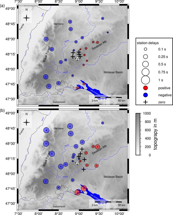
1390                                                              S. Mader et al.: Seismicity and seismotectonics of the ASZ

tended (Stange, 2018), and in summer 2015 the installa-            the Swabian Alb forms a typical cuesta landscape with ma-
tion of the temporary Alp Array Seismic Network (AASN)             jor escarpments built up by resistant carbonates of the Late
started (Hetényi et al., 2018). In 2018 we started our project     Jurassic that is cut by several large fault systems, which are
StressTransfer, in which we investigate areas of distinct seis-    detectable in the present-day topography (Reicherter et al.,
micity in the northern Alpine foreland of southwestern Ger-        2008). The Black Forest to the west of the Swabian Alb ex-
many and the related stress field (Mader and Ritter, 2021).        perienced the most extensive uplift due to the extension of
The StressTransfer network consist of 15 seismic stations,         the URG. Here, even metamorphic and magmatic rocks of
equipped with instruments of the KArlsruhe BroadBand Ar-           the Paleozoic basement are exposed. To the north and north-
ray (KABBA), in our research area (Fig. 1a).                       west of the Swabian Alb, Triassic rocks crop out (Meschede
   Here we present a compilation of different data sets to         and Warr, 2019). Due to the different uplift and erosional
refine hypocentral parameters of the ASZ. For this we an-          states of southern Germany, the depth of the crystalline base-
alyze the earthquake catalog of the LED from 2011 to 2018          ment varies strongly between −5.4 and 1.2 km a.s.l. (Rupf
(Bulletin-Files des Landeserdbebendienstes B-W, 2018) and          and Nitsch, 2008).
complement it with additional phase picks from recordings              The current regional stress field of southwestern Germany
of AASN (AlpArray Seismic Network, 2015) and our own               is dominated by an average horizontal stress orientation of
StressTransfer seismic stations. We calculate a new 1-D seis-      150◦ (e.g., Müller et al., 1992; Plenefisch and Bonjer, 1997;
mic velocity model and relocate the events. For several relo-      Reinecker et al., 2010; Heidbach et al., 2016) and was de-
cated events we calculate fault plane solutions. This proce-       termined from focal mechanism solutions, overcoring, bore-
dure gives us a new view of the geometry of the fault pat-         hole breakouts and hydraulic fracturing (e.g., Bonjer, 1997;
tern at depth in the ASZ based on its microseismic activity.       Plenefisch and Bonjer, 1997; Kastrup et al., 2004; Reiter et
Furthermore, we use the fault plane solutions to derive the        al., 2015; Heidbach et al., 2016). It is characterized by NW–
orientation of the main stress components in the area of the       SE horizontal compression and NE–SW extension (e.g., Kas-
ASZ and discuss these with known results.                          trup et al., 2004) and developed during late Miocene (Becker,
                                                                   1993). Analysis of several kinematic indicators hint that fault
                                                                   planes where already activated repeatedly during the Ceno-
2   Geological and tectonic setting                                zoic (Reicherter et al., 2008). Three main groups of fault
                                                                   planes can be observed. First, mainly sinistral NNE–SSW-
Southwestern Germany is an area of low to moderate seis-           to-N–S-striking fault planes, which are similar to the ASZ
micity. The most active fault zones are the Upper Rhine            or the Lauchert Graben (Fig. 1b) and parallel the URG. Sec-
Graben (URG) and the area of the ASZ and the Hohenzollern          ond, NW–SE-striking normal and/or dextral strike-slip fault
Graben system (HZG, Fig. 1b). In the region of the URG,            planes, which correspond to the HZG in our area. Older kine-
the seismicity is distributed over a large area. In comparison,    matic indicators, like fiber tension gashes and stylolites, hint
in our research area the seismicity clusters in the close area     at a sinistral initiation of those NW–SE striking fault planes
around the ASZ and the HZG.                                        during the Late Cretaceous–Paleogene with a maximum hor-
   The ASZ is named after the town of Albstadt, situated on        izontal compression in the NE–SW direction (Reicherter et
the Swabian Alb, a mountain range in southern Germany              al., 2008). Third, ENE–WSW-oriented fault planes, which
(Fig. 1a). Southern Germany consists of several tectono-           are mainly inactive but with some exhibiting dextral strike-
stratigraphic units, a polymetamorphic basement with a             slip or reverse movement, for example, the Swabian Line
Mesozoic cover tilted towards southeast to east due to ex-         (Schwäbisches Lineament, Fig. 1b). The direction of SHmax
tension in the URG (Fig. 1c), associated with updoming             in our research area is quite constant, except of an area di-
(Reicherter et al., 2008; Meschede and Warr, 2019). The            rectly south of the HZG (Albstadt-Truchtelfingen) and within
URG forms the western tectonic boundary, whereas the east-         the HZG (Albstadt-Onstmettingen). There the SHmax direc-
ern boundary comprises the crystalline basement of the Bo-         tion rotates about 20◦ counterclockwise into the strike of the
hemian Massif. To the south, the foreland basin of the Alps        HZG (130◦ , Baumann, 1986), which may be caused by a re-
(Molasse Basin, Fig. 1c) frames the area in a triangular           duced marginal shear resistance.
shape. The Molasse Basin covers the whole area south of                The only morphologically visible tectonic feature close to
the Swabian Alb up to the Alpine mountain chain. It is filled      Albstadt is the HZG (Fig. 1b), a small graben with an inver-
with Neogene terrestrial, freshwater and shallow marine sed-       sion of relief and a NW–SE strike (Schädel, 1976; Reinecker
iments (Fig. 1c, Meschede and Warr, 2019). The Swabian             and Schneider, 2002). The 25 km long HZG has dip angles
Alb is bounded by the rivers Neckar in the north and Danube        between 60–70◦ at the main faults and a maximum graben
in the south (Fig. 1a). The sedimentary layers of the Swabian      width of 1.5 km, which leads to a convergence depth of the
Alb, which consist of Jurassic limestone, marl, silt and clay,     main faults in 2–3 km depth (Schädel, 1976). Thus, the HZG
dip downwards by 4◦ to the southeast and disappear be-             is interpreted as a rather shallow tectonic feature. To the north
low the Molasse Basin (Fig. 1c) and the Alpine mountain            and south of Albstadt there are further similar graben struc-
chain (Meschede and Warr, 2019). The sedimentary cover of          tures like the HZG, namely the Filder Graben, Rottenburg

Solid Earth, 12, 1389–1409, 2021                                                       https://doi.org/10.5194/se-12-1389-2021
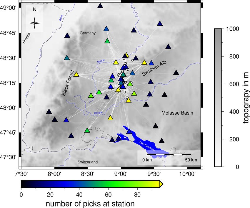
S. Mader et al.: Seismicity and seismotectonics of the ASZ                                                                            1391

Figure 1. (a) Overview over our research area located in southwestern Germany in the northern Alpine foreland. The ASZ is our research tar-
get (framed area). Black triangles represent permanent seismic stations of the LED and other agencies. Yellow triangles represent temporary
AlpArray seismic stations. Green triangles display the 15 temporary seismic stations of the StressTransfer network. The gray circles display
the seismicity scaled by magnitude from 2011 to 2018. URG stands for Upper Rhine Graben. (b) Close-up of the area of the ASZ (framed
area in (a)). Symbols are the same as in (a). The red-framed triangle highlights the central station Meßstetten (MSS) of the minimum 1-D
seismic velocity model. White stars mark epicenters of the four strongest events, which had a magnitude greater than 5 in 1911, 2 in 1943
(same epicenter) and 1978, as well as the earthquake on 22 March 2003 with a local magnitude of 4.4 (Leydecker, 2011) these events are
not included in the earthquake catalog from 2011 to 2018 (gray circles scaled with magnitude like in Fig. 1a). White lines indicate known
and assumed faults (Regierungspräsidium Freiburg, 2019). The Hohenzollern Graben (HZG) is the only clear morphological feature in the
close vicinity of the ASZ. Other large tectonic features are the Lauchert Graben (LG) and the Swabian Line (SL). Topography is based on the
ETOPO1 Global Relief Model (Amante and Eakins, 2009; NOAA National Geophysical Data Center, 2009). (c) Overview on the geology
of the research area region; geology data are taken from Asch (2005). Topography is based on SRTM15+ (Tozer et al., 2019).

https://doi.org/10.5194/se-12-1389-2021                                                              Solid Earth, 12, 1389–1409, 2021
1392                                                                S. Mader et al.: Seismicity and seismotectonics of the ASZ

Flexure, western Lake Constance faults and Hegau, which              land, with a further three earthquakes with a local magnitude
are also about parallel to the main horizontal stress field (Rei-    greater than 5 (Fig. 1b, 2 events in 1943, 1978, e.g., Rei-
necker et al., 2010) like the HZG. Reinecker and Schneider           necker and Schneider, 2002; Stange and Brüstle, 2005). The
(2002) propose a tectonic model to relate the graben struc-          latest strong events occurred on 4 November 2019 (ML 3.8),
tures with the ASZ below. They apply the result of Tron              27 January 2020 (ML 3.5) and 1 December 2020 (ML 4.4,
and Brun (1991), who showed that the movement of a partly            Regierungspräsidium Freiburg, 2020). The average seismic
decoupled strike-slip fault in the subsurface can generate           dislocation rates along the ASZ are on the order of 0.1 mm/a,
graben structures at the surface in a steplike arrangement.          respectively (Schneider, 1993). The return period of earth-
In the regional tectonic model, the graben structures are the        quakes along the ASZ with a magnitude of 5 is approxi-
HZG, the Rottenburg Flexure, western Lake Constance faults           mately 1000 years (Schneider, 1980; Reinecker and Schnei-
and the Filder Graben (Reinecker and Schneider, 2002). The           der, 2002). Both estimates are based on historic earthquake
ASZ itself is the strike-slip fault, partly decoupled from the       records. From aftershock analyses and focal mechanism cal-
surface by a layer of Middle Triassic evaporites in the over-        culations we know that the ASZ is a steep NNE–SSW-
lying sedimentary layers (Reinecker and Schneider, 2002).            oriented sinistral strike-slip fault (e.g., Haessler et al., 1980;
Stange and Brüstle (2005) consider the bottom of the Meso-           Turnovsky, 1981; Stange and Brüstle, 2005) in the crystalline
zoic sediments a mechanical decoupling horizon as no earth-          basement, as all earthquakes occur at a depth greater than
quakes occur above 2 km depth.                                       2 km (Stange and Brüstle, 2005). The lateral extent of the
    Another tectonic feature in our research area is the ENE–        fault zone in an N–S direction is still under debate: Reinecker
WSW-striking Swabian Line north of the river Neckar                  and Schneider (2002) propose an extension from northern
(Fig. 1b). It extends from the Black Forest area partly parallel     Switzerland towards the north of Stuttgart, whereas Stange
along the cuesta of the Swabian Alb to the east (Reicherter et       and Brüstle (2005) do not find this large extension as most of
al., 2008). The sense of movement along the Swabian Line             the seismicity happens on the Swabian Alb.
is dextral. To the east of the ASZ near Sigmaringen, the
Lauchert Graben strikes N–S, about parallel to the ASZ with
a sinistral sense of displacement (Geyer and Gwinner, 2011,          3   Earthquake data and station network
Fig. 1b).
    The faults in southwestern Germany exhibit mainly mod-           As a basis for our study, we use the earthquake catalog
erate displacements during the last ca. 5 Myr (Reicherter et         of the LED from 2011 to 2018 for earthquakes within the
al., 2008). At the HZG, for example, the maximum verti-              area close to the ASZ (8.5–9.5◦ E, 48–48.8◦ N, Fig. 1b).
cal offset is of the order of 100–150 m. The horizontal offset       For these 575 earthquakes we received the bulletin files of
is considerably lower and more difficult to determine (Re-           the LED (Bulletin-Files des Landeserdbebendienstes, B-W,
icherter et al., 2008).                                              2018), consisting of hypocenter location, origin time, local
    Along the 9◦ E meridian Wetzel and Franzke (2003) iden-          magnitude ML, and all phase travel time picks with corre-
tified a 5–10 km broad zone of lineations pursuable from             sponding quality and P-phase polarity. The LED picks from
Stuttgart to Lake Constance (Fig. 1a). Those lineations strike       2011 to 2018 are from 51 LED seismic stations and 14 seis-
predominantly N–S, NW–SW and ENE–WSW. The N–S-                       mic stations run by other agencies like the state earthquake
and ENE–WSW-striking faults limited the NW–SE-striking               service of Switzerland (Fig. 1a). Locations are determined
graben structures like the HZG (Reicherter et al., 2008). The        with HYPOPLUS, a Hypoinverse variant modified follow-
NW–SE-striking faults are expected to be possibly active at          ing Oncescu et al. (1996), which allows the usage of a 1.5-D
intersections with N–S-striking faults due to a reduction in         seismic velocity model approach (Stange and Brüstle, 2005).
shear resistance accompanied by aseismic creep (Schneider,           Most hypocenter depths are well determined, but around
1979, 1993; Wetzel and Franzke, 2003).                               9.7 % of the depth values are manually fixed. The median
    The first documented earthquakes in the area of the ASZ          uncertainties for longitude, latitude and depth within the cat-
occurred in 1655 near Tübingen and had an intensity of 7 to          alog are 0.5, 0.6 and 2.0 km, respectively. The magnitude ML
7.5 (Leydecker, 2011). A similarly strong earthquake with            ranges from 0.0 to 3.4, with average uncertainties of about
a local magnitude of 6.1 occurred in 1911 near Albstadt-             ±0.2, and the magnitude of completeness is around ML 0.6
Ebingen (Fig. 1b, Leydecker, 2011), causing damage to                (see Fig. S1 in the Supplement). The catalog used only con-
buildings (Reicherter et al., 2008). The seismic shock trig-         tains natural events, as quarry blasts are sorted out and in-
gered landslides with surface scarps in both the superfi-            duced events do not occur in the study region.
cial Quaternary deposits and the Tertiary Molasse sediments             Additionally, within the AlpArray Project (Hetényi et al.,
(Sieberg and Lais, 1925) in the epicentral area and close to         2018), nine seismic stations were installed starting in sum-
Lake Constance, demonstrating the potential of hazardous             mer 2015 within 80 km distance to the ASZ, four of them
secondary earthquake effects (Reicherter et al., 2008). Since        directly around the ASZ (AlpArray Seismic Network, 2015,
the 1911 earthquake, the Swabian Alb has been one of the             Fig. 1b). To get an even denser network and to detect mi-
most seismically active regions in the northern Alpine fore-         croseismicity we started to install another 15 seismic broad-

Solid Earth, 12, 1389–1409, 2021                                                         https://doi.org/10.5194/se-12-1389-2021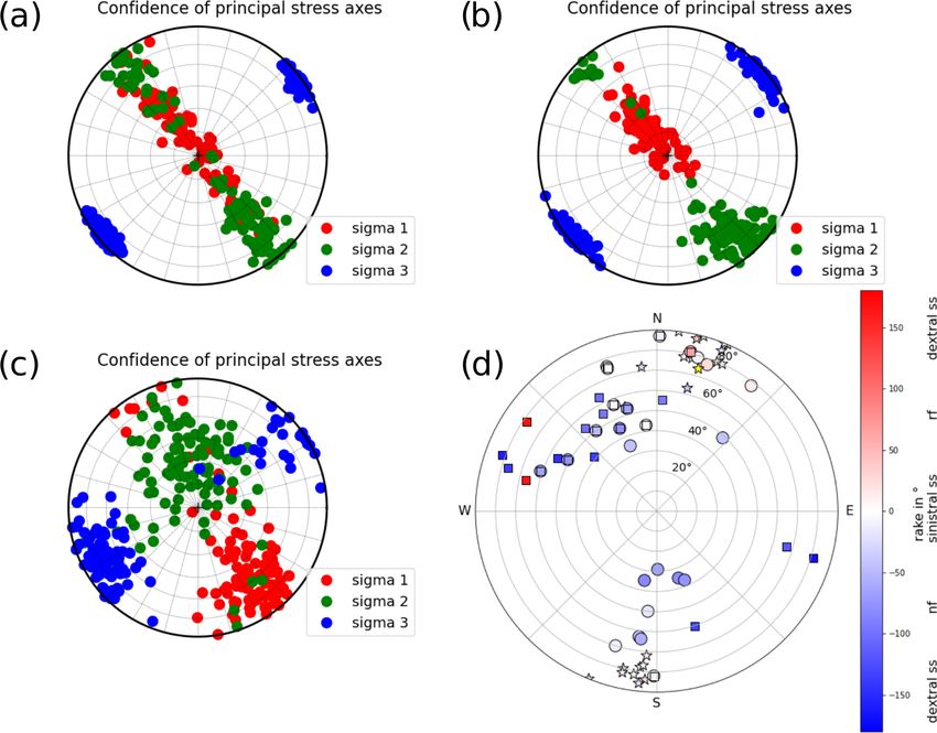
S. Mader et al.: Seismicity and seismotectonics of the ASZ                                                                       1393

band stations from the KABBA beginning in July 2018 in
areas with striking seismicity in the northern Alpine foreland
within our project StressTransfer (Fig. 1a) (Mader and Ritter,
2021). Five of those stations are located in the vicinity of the
ASZ (Fig. 1b), and three of them where already running at
the end of 2018.
   We complemented the LED catalog with additional seis-
mic P- and S-phase picks from the four AASN stations
located around the ASZ from 2016 to 2018 and our
StressTransfer stations recording in 2018. In total, our com-
bined data set consists of 575 earthquakes (Fig. 1b) with
4521 direct P-phase and 4567 direct S-phase travel time picks
from 69 seismic stations.

4     Data processing

4.1    Phase picking                                               Figure 2. Ray coverage and input data set for the inversion with
                                                                   VELEST. White circles represent the 99 selected events that are
To complement the LED catalog, we use a self-written code          used for vp and vs inversion. Seismic stations are indicated as tri-
in ObsPy (e.g., Beyreuther et al., 2010) for semi-automatic        angles and color-coded with the number of high-quality picks at a
manual picking of the direct P and S phases. The raw               station used for the vp and vs inversion. Topography is based on the
waveform recordings are bandpass-filtered with a zero-phase        ETOPO1 Global Relief Model (Amante and Eakins, 2009; NOAA
four corners Butterworth filter from 3 to 15 Hz. Using the         National Geophysical Data Center, 2009).
hypocenter coordinates of the LED we calculate an approx-
imate arrival time at a seismic station. Around this arrival
time, we define a noise and a signal time window follow-              To determine a complemented catalog, we invert for new
ing Diehl et al. (2012) so that we can calculate the signal to     minimum 1-D seismic vp and vs models in the region of the
noise ratio (SNR) of our phase onsets. Our code automati-          ASZ with station delay times, using the program VELEST
cally calculates the earliest possible pick (ep) and the latest    (Kissling et al., 1994, 1995, VELEST Version 4.5). As cen-
possible pick (lp) (see Diehl et al., 2012) to get consistent      tral recording station we chose the station Meßstetten (MSS,
error boundaries for each pick. Finally, the error boundaries      Fig. 1b), as this station was running during our complete ob-
are checked by eye, and the phase pick is done manually be-        servational period and it is the oldest seismic recording site
tween the two error boundaries. The qualities of 0 up to 4         on the Swabian Alb, having been recording since 2 June 1933
of the picked arrival time are set depending on the time dif-      (Hiller, 1933). To get the best subset of our catalog for the
ference between ep and lp (Table A1 in the Appendix). For          inversion, we select only events with at least eight P-arrival
consistency, a similar relationship is used between picking        times for the inversion for vp and either eight P-arrival or
quality and uncertainty as defined by the LED (Bulletin-Files      eight S-arrival times for the simultaneous inversion for vp
des Landeserdbebendienstes B-W, 2018).                             and vs . The P-pick times exhibit a quality of 1 or better, and
                                                                   the S-picks need a quality of 2 or better (Table A1). Events
4.2    Inversion for minimum 1-D seismic velocity models           outside of the region of interest, 48.17–48.50◦ N and 8.75–
       with VELEST                                                 9.15◦ E, with an azimuthal GAP greater than 150◦ and an
                                                                   epicentral distance of more than 80 km are rejected. This se-
The LED uses the program HYPOPLUS (Oncescu et al.,                 lection leads to a high-quality subset of 68 events with 789
1996) for routine location, with which one can apply a 1.5-        P-phase picks for vp and 99 events with 945 P-picks and 1019
D approach by using several 1-D seismic velocity models            S-phase picks for the vp and vs inversion (Fig. 2).
for selected regions (Stange and Brüstle, 2005; Bulletin-Files        To probe our seismic velocity model space, inversions with
des Landeserdbebendienstes B-W, 2018). They use two P-             84 different starting models are calculated with four differ-
wave velocity (vp ) models, a Swabian Jura model and a             ently layered models from seismic refraction profile interpre-
model for the state of Baden-Württemberg, and they define          tations (Gajewski and Prodehl, 1985; Gajewski et al., 1987;
the S-wave velocity (vs ) model using a constant vp /vs ra-        Aichroth et al., 1992), the LED Swabian Jura model (Stange
tio (Stange and Brüstle, 2005; Bulletin-Files des Landeserd-       and Brüstle, 2005) and realistic random vp variations (Fig. 3).
bebendienstes B-W, 2018, Fig. 4a, b). Furthermore, no sta-         We apply a staggered inversion scheme following Kissling et
tion delay times are used (Bulletin-Files des Landeserd-           al. (1995) and Gräber (1993), first inverting for vp and then
bebendienstes B-W, 2018).                                          for vp and vs together while damping the vp model. The in-

https://doi.org/10.5194/se-12-1389-2021                                                        Solid Earth, 12, 1389–1409, 2021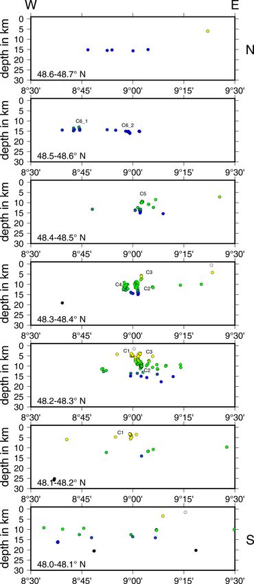
1394                                                                   S. Mader et al.: Seismicity and seismotectonics of the ASZ

                                                                        indicates that the model represents the data and region very
                                                                        well and that the determined hypocenter locations are stable.
                                                                           We calculated an error estimate based on the variation of
                                                                        the 21 output vp and vs models with our chosen layer model
                                                                        of Gajewski et al. (1987) for ASZmod1 (Table 1). For a pre-
                                                                        cise estimation we determined 2 times the standard deviation
                                                                        (2σ ) of the velocity models for each layer. For the uppermost
                                                                        layer we could not estimate any error, as the first layer was
                                                                        manually set and strongly damped during the inversion pro-
                                                                        cess. The 2σ range is small for the third and fourth layers.
                                                                        This was expected as most of the events are located within
                                                                        those layers and as all other models (which also have dif-
                                                                        ferent layering) converge to similar velocities in those layers
                                                                        (Fig. 3). The error estimate for the second layer has to be
Figure 3. VELEST input models for vp (84) and vs (21) (gray)            considered carefully as this layer revealed strong instabili-
and output vp (84) and vs (21) after inversion (black) together with    ties during the stability test (Fig. S3). The fifth layer also
the chosen model ASZmod1 (colored). A good convergence of the           has larger 2σ uncertainties relative to layers three and four,
models can be observed, especially for vs . The second layer con-       which is caused by less ray coverage and there being no
verges worst. An instability of the first layer with a tendency to      events located below 18.25 km depth.
unrealistic low seismic velocities can be seen. For this reason, the
velocity of ASZmod1 was fixed in the first layer.
                                                                        4.3   Relocation, station corrections and error
                                                                              estimation with NonLinLoc

version for vp was done with the 84 different starting mod-             To relocalize the complete earthquake catalog we use the
els described previously, always using the resulting veloc-             program NonLinLoc (NLL, Lomax et al., 2000), a nonlin-
ity model of the prior inversion as input for the next inver-           ear oct-tree search algorithm. NLL calculates travel time ta-
sion with VELEST. After three to four inversion runs, the               bles following the eikonal finite-difference scheme of Pod-
velocity models converged, and the results did not change               vin and Lecomte (1991) on a predefined grid, here using
(Fig. 3). Following this, the inversion for station delay times         1 km grid spacing. With the implemented oct-tree search al-
was done. The minimum 1-D vp model with the smallest rms                gorithm, (density) plots of the probability density function
and the simplest layering was selected as the final vp model            (PDF) of each event are determined following the inversion
for the simultaneous vp and vs inversion. Together with a               approach of Tarantola and Valette (1982) with either the L2-
vp /vs ratio of 1.69 (Stange and Brüstle, 2005), it was also            rms likelihood function (L2) or the equal differential time
used to calculate the vs starting model, which was randomly             likelihood function (EDT). The determined PDF contains lo-
changed to get a total of 21 vs starting models (Fig. 3). The           cation uncertainties due to phase arrival time errors, theo-
inversion was done like the staggered inversion for vp . The            retical travel time estimation errors and the geometry of the
resulting minimum 1-D vp and vs models (ASZmod1, Fig. 4)                network (Husen et al., 2003). Based on the PDFs an error el-
were selected due to their small rms.                                   lipsoid (68 % confidence) is determined, which we use to cal-
   To test the stability of ASZmod1, we randomly shifted all            culate latitude, longitude and depth error estimates for each
99 events in space by maximum 0.1◦ horizontally and 5 km                earthquake (Fig. 5). The estimated errors of our events (es-
with depth (Kissling et al., 1995). The result of this shift test       pecially the depth error estimate) have been getting smaller
demonstrates that we can determine stable hypocenters, with             since 2016. This reduction correlates well with the increased
an average deviation of less than 0.005◦ horizontally and of            number of picks per event and thus with the increased num-
less than 2 km in depth for more than 90 % of the events in             ber of seismic stations around the ASZ due to the modifica-
the catalog (Fig. S2). The seismic velocities are stable, except        tion of the LED network and the installation of the AASN
for the first and second layer (Fig. S3a, b). The first layer was       and the StressTransfer stations from 2018 (Hetényi et al.,
unstable already during the inversion process (Fig. 3); there-          2018; Stange, 2018, Fig. 5). As a final hypocenter solution
fore, we damped its layer velocities and set them to realistic          the maximum likelihood hypocenter is selected, which cor-
vp and vs values based on the seismic vp of the refraction pro-         responds to the minimum of the PDF.
file interpretations (Gajewski et al., 1987). The instability in           We compared the resulting hypocenters and error esti-
both upper layers may be caused by few refracting rays and              mates using the L2 or the EDT likelihood function. The com-
thus small horizontal ray lengths through the layers. Further-          parison mainly indicates similar earthquake locations, but we
more, there are only a few earthquakes located within these             find EDT errors (Fig. S4) for many events that are too large
layers (Fig. S3c). In total, the stability test (Figs. S2 and S3)       and that are unrealistic (some greater than 50 km, leading to

Solid Earth, 12, 1389–1409, 2021                                                           https://doi.org/10.5194/se-12-1389-2021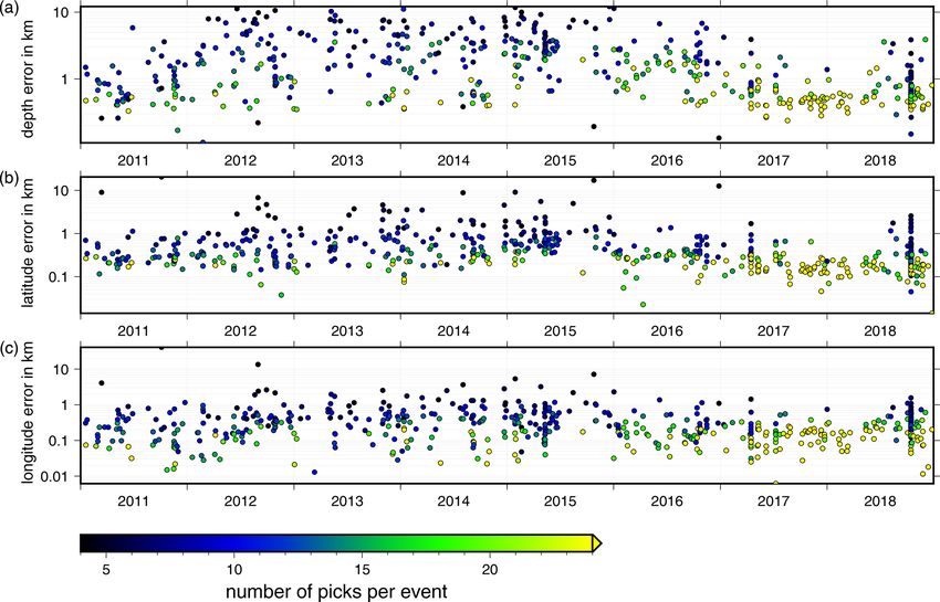
S. Mader et al.: Seismicity and seismotectonics of the ASZ 1395
Table 1. ASZmod1 with corresponding error estimates based on 2σ .
Layer top in km vp in km/s 2σ vp in km/s vs in km/s 2σ vs in km/s
Layer 1 −2 3.47 – 1.98 –
Layer 2 0.1 5.06 0.30 2.90 0.06
Layer 3 2.5 5.68 0.03 3.37 0.01
Layer 4 5.63 5.95 0.02 3.57 0.01
Layer 5 18.25 6.55 0.31 3.91 0.32
Figure 4. (a) Final minimum 1-D seismic velocity models (ASZmod1): vs is in green, and vp is in blue. Gray lines represent velocity models
of the LED (Bulletin-Files des Landeserdbebendienstes B-W, 2018): solid lines show Swabian Jura models, and dashed lines show Baden-
Württemberg models. Red bars are scaled with the number of events in each layer of the velocity model. (b) vp /vs ratio of ASZmod1 and the
LED models. (c) Ray statistics of used ray paths. Red bars display number of hits per layer. Blue and green lines give the average horizontal
and vertical ray length.
hypocenter shifts across the whole region). For this reason, (Quality 0, Table A1), we consider the station delay times of
we decided to use L2 for relocating our combined catalog. MSS to be practically zero. To account for similar small sta-
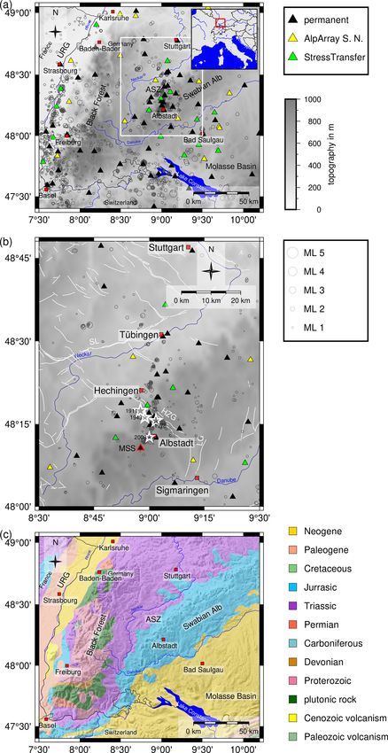
In NLL one can examine station delay times calculated tion delay times and σ , we state that all station delay times in
from the station residuals. The station delay times are de- the range of −0.05 to 0.05 s are practically zero station delay
fined as the time correction subtracted from the observed P- times if σ is greater than the actual station delay time (Fig. 6).
and S-wave arrival times. This implies that negative station The fact that the NLL station delay times of MSS and sur-
delay times exhibit faster velocities relative to ASZmod1 and rounding stations are close to zero indicates that even though
positive station delay times exhibit slower velocities relative they use a different (and nonlinear) relocation algorithm for
to ASZmod1. We used ASZmod1 and the corresponding VE- delay time estimation than VELEST, our determined mini-
LEST station delay times, as well as our high-quality subset mum 1-D seismic velocity model ASZmod1 represents the
of 99 earthquakes, as input for NLL. After four iterative runs seismic velocity structure below MSS and its surroundings
of NLL, always using the output station delay times as new very well.
input station delay times, the determined station delay times We compared the relocated catalog with the original LED
become stable. As we want to relocate the whole catalog with locations. Some events have large differences in hypocen-
NLL, we use the NLL updated VELEST station delay times ter coordinates (> 0.1◦ in latitude or longitude), which we
for consistency. Since ASZmod1 is a 1-D seismic velocity identified as events with only a few arrival time picks (fewer
model below the reference station MSS, we expect the sta- than nine picks), a large azimuthal GAP (GAP > 180◦ ) or
tion delay times to become zero for MSS. After four itera- wrong phase picks. Furthermore, a large deviation of expec-
tive runs the actually determined station delay times of MSS tation and maximum likelihood hypocenters indicates an ill-
are 0.014 s with σ of 0.083 s for vp and −0.027 s with σ of conditioned inverse problem with a probable non-Gaussian
0.064 s for vs . As σ is bigger than the actual station delay distribution of the PDF (Lomax et al., 2000), which was the
time and the station delay time of MSS is smaller than the case for some events with only a few picked arrival times.
maximum error range of 0.05 s of our best determined picks Similar problems were also identified by Husen et al. (2003),
https://doi.org/10.5194/se-12-1389-2021 Solid Earth, 12, 1389–1409, 2021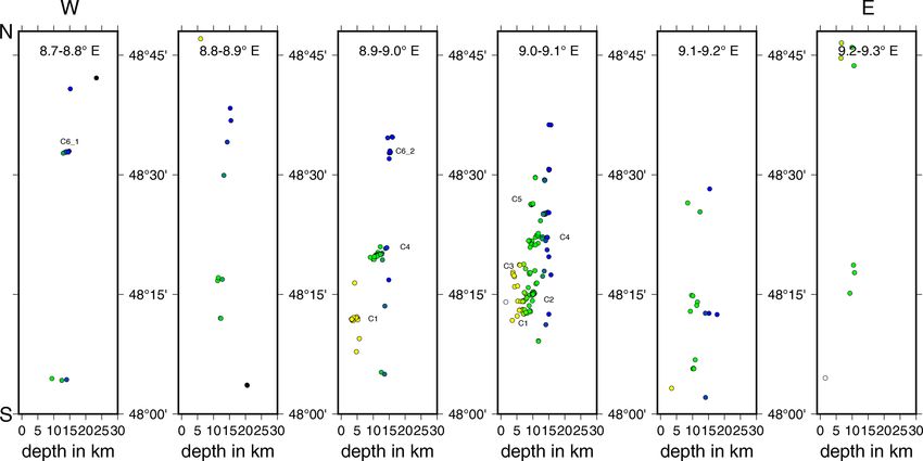
1396                                                                    S. Mader et al.: Seismicity and seismotectonics of the ASZ

Figure 5. Errors calculated from the 68 % confidence ellipsoid from NLL with L2 (L2-rms likelihood function) for each event in the combined
catalog for (a) depth, (b) latitude and (c) longitude. The errors are color-coded depending on the number of picks, with dark colors indicating
fewer picks and bright colors indicating many picks. Hypocenters with many observations are determined with smaller errors in depth and
lateral position.

who compared NLL locations with the routine locations of                  4.4   Focal mechanism models with FOCMEC
the state earthquake service of Switzerland. They also found
that a good depth estimate with NLL depends on the sta-
tion’s distance from the earthquake. Especially for events                We determine fault plane solutions for 25 selected events
with many observations, the depth estimate was worse if the               with the program FOCMEC (Snoke, 2003), which conducts
closest station was further away than the focal depth of the              a grid search over the complete focal sphere and outputs all
event (Husen et al., 2003).                                               possible fault plane solutions. For this we used the P-polarity
   Our well-located earthquakes are selected by the follow-               picks of the LED (Bulletin-Files des Landeserdbebendien-
ing criteria: more than eight travel time picks, a GAP less               stes B-W, 2018), and for events since 2016 we added P and
than 180◦ , a horizontal error estimate of less than 1 km and a           SH polarities, as well as SH / P amplitude ratios, at the four
depth error estimate of less than 2 km (Fig. 7). Some of our              AASN and three StressTransfer seismic stations. The local
well-located events have quite different depth estimates com-             magnitude ML of those 25 events is in the range 0.6 to 3.4
pared to the LED solution (Fig. S5). Thus, we checked the                 (Table 2, Fig. 7, Bulletin-Files des Landeserdbebendienstes
station distribution for those events as proposed by Husen et             B-W, 2018).
al. (2003) and looked for incorrect phase picks. Nevertheless,                To determine the SH / P amplitude ratios we only used
all of these events have good phase picks, a small depth er-              SH- or P-picks with a quality of 2 or better and the SNR
ror estimate, evenly distributed stations and small deviations            of the picked phase needed to be greater than 5. Further-
of expectation and maximum likelihood hypocenter coordi-                  more, we compared the frequency content of the P and SH
nates. For this reason, we consider our new depth locations               phase to assure that the waves have the same damping prop-
well determined and reliable.                                             erties, and the the source process was simple (Snoke, 2003).
   In comparison with the LED catalog, the majority of our                If the determined frequency of P and SH phases differed
relocated earthquakes are characterized by a small eastward               by more than 5 Hz the SH / P amplitude ratio was omit-
shift and a stronger clustering, especially in depth (Fig. S5).           ted. All waveforms are instrument-corrected and bandpass-
The latter may result from the hand-set depth location for                filtered between 1 and 25 Hz. As FOCMEC uses the ratio on
some events of the LED.                                                   the focal sphere we need to correct our amplitudes for atten-
                                                                          uation effects and phase conversion effects at the free surface
                                                                          (Snoke, 2003). To correct for attenuation effects we use QP
                                                                          and QS values determined by Akinci et al. (2004) for south-
                                                                          ern Germany. The measured phase amplitude A depends on

Solid Earth, 12, 1389–1409, 2021                                                               https://doi.org/10.5194/se-12-1389-2021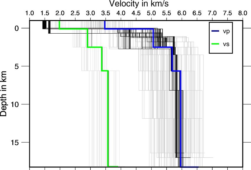
Table 2. Parameters of the FOCMEC solutions. Values with (aux) refer to the assumed auxiliary plane.

                                           ID                  Time    ML      ◦N     ◦E    Depth    P   SH   SH / P   Strike   Dip    Rake    1strike   1dip    1rake    Strike(aux)    Dip (aux)    Rake (aux)    Quality
                                                                                            in km                        in ◦   in ◦    in ◦      in ◦    in ◦     in ◦           in ◦         in ◦          in ◦
                                           ev335   2016-04-10T15:08    1.1   48.44   9.05    9.44    8    3        0     353     43     −5        7.6     9.7     14.5            87            87         −133          1
                                           ev353   2016-09-02T07:58    2.2   48.20   9.00    5.09   14    3        0      12     81     65        0.0     0.0      0.0           263            26          159          0

https://doi.org/10.5194/se-12-1389-2021
                                           ev364   2016-10-13T01:54    1.0   48.34   8.96   11.45    9    2        1     338     35    −43       46.1    50.0     57.8           105            67         −117          4
                                           ev378   2016-12-07T20:55    1.4   48.61   8.87   15.46    8    2        2     181     82     −5       14.2    18.8     68.2           272            85         −172          4
                                           ev402   2017-04-15T17:16    2.1   48.33   8.96   11.15   17    4        1     162     35    −81        0.0     0.0      0.0           331            55          −96          0
                                           ev405   2017-05-07T15:19    0.6   48.30   9.10   10.65   10    3        1      42     49    −41       56.8    35.4     41.8           162            60         −131          4
                                           ev423   2017-07-09T11:52    0.8   48.33   8.96   11.36    8    4        0     158     37    −75       22.0    11.4     29.6           319            54         −101          2
                                           ev426   2017-07-23T13:48    1.4   48.44   9.04   10.03   14    3        0       1     87    −10        0.0     0.0      0.0            92            80         −177          0
                                           ev432   2017-08-27T06:00    1.7   48.20   8.87   12.18   29    4        0      37     78     12        3.1    17.3      7.6           304            78          168          1
                                           ev457   2018-02-10T12:44    2.3   48.33   8.95   12.41   27    3        2     197     70     −9        2.0     6.9     19.0           290            82         −160          1
                                                                                                                                                                                                                              S. Mader et al.: Seismicity and seismotectonics of the ASZ

                                           ev463   2018-03-13T05:14    1.0   48.20   8.99    3.30   11    3        1      15     79     −9       26.9    31.9     63.3           107            81         −169          4
                                           ev514   2018-10-15T18:46    0.8   48.25   9.04   10.35    8    4        1     289     61    −65       23.3    15.5     31.6            65            38         −127          3
                                           ev522   2018-10-15T19:37    1.3   48.25   9.04   10.00   17    4        3     341     76     −1        2.8     6.8     10.2            71            89         −166          1
                                           ev525   2018-10-15T19:41    1.6   48.25   9.04   10.08   27    4        4     341     75     −4        3.8     8.0     12.0            72            86         −165          1
                                           ev552   2018-10-17T03:02    1.0   48.25   9.04   10.38   14    4        2     338     57     −7        9.3    32.0     11.4            72            84         −147          3
                                           ev554   2018-10-24T07:12    1.7   48.27   9.03    5.22   23    4        2     185     50    −17        5.2    14.8      0.6           286            77         −139          1
                                           ev561   2018-11-18T16:23    1.6   48.60   8.65   14.44   10    3        0     336     45    −78       22.0    25.4     32.4           139            46         −102          3
                                           ev564   2018-11-25T02:22    1.4   48.25   9.04   10.20   25    3        2     344     53    −65        0.0     0.0      0.0           126            44         −119          0
                                           ev565   2018-11-25T07:36    0.9   48.25   9.04   10.24   21    2        0     190     35    −84       32.3    40.1     12.2             3            55          −94          4
                                           ev566   2018-11-25T10:25    0.9   48.25   9.04   10.22   13    5        1     323     50    −45       35.3    15.6     14.5            86            57         −130          3
                                           ev171   2013-12-04T19:42    2.9   48.31   9.04    5.76   13    0        0     188     63    −39       11.4    41.3     44.7           298            56         −147          4
                                           ev183   2014-01-12T23:45    1.3   48.04   8.63   16.29   12    0        0     187     64    −57       42.7    34.9     37.2           311            41         −138          4
                                           ev221   2014-09-09T00:46    2.3   48.21   9.12    9.31   14    0        0     179     29    −67       47.3    59.2     44.8           333            64         −102          4
                                           ev232   2014-10-24T02:09    2.0   48.35   9.02    9.11   11    0        0     300     51    −76       53.8    39.9     38.5            98            41         −107          4
                                           ev245   2015-01-28T00:05    3.4   48.20   8.99    4.99   19    0        0      19     77     24        5.3    18.5     61.3           283            67          166          4

Solid Earth, 12, 1389–1409, 2021
                                                                                                                                                                                                                              1397
1398 S. Mader et al.: Seismicity and seismotectonics of the ASZ
Q, the frequency of the phase f , the travel time t and the
amplitude A0 at the source (e.g., Aki and Richards, 1980):
ft
A = A0 e−π Q . (1)
The correction factor for the free surface effect of SH waves
is always 2 and independent of the incidence angle of the
seismic wave. For the P wave the free surface correction
strongly depends on the incidence angle and the vp /vs ratio
(e.g., Aki and Richards, 1980). We calculated the incidence
angle for our P phases of interest with the TAUP package of
ObsPy (e.g., Beyreuther et al., 2010) using the AK135 model
(Kennett et al., 1995) and find incidence angles in a range
between 22.9 and 23.2◦ . As the variation between the inci-
dence angles for the different station event combinations is
very small, we use for all events the median incidence angle
of 23.05◦ . To calculate the vp /vs ratio, we use vp and vs of
the second layer of our model ASZmod1 (Table 1) because
in the first layer the velocities are considered to be unstable.
After this correction the logarithm of the SH / P amplitude
ratio is used as input in FOCMEC together with the P and
SH polarities.
To find the appropriate solution one can allow different
types of errors in FOCMEC. We compare the relative weight-
ing mode and the unity weighting mode of the FOCMEC in-
version for all events. This is done to explore if the results
differ significantly, which could mean that they are question- Figure 6. (a) Station delay times for the vp velocity model ASZ-
able (Snoke, 2003). In the unity weighting mode each wrong mod1. (b) Station delay times for the vs velocity model ASZmod1.
polarity in the FOCMEC solution counts as an error of 1. Blue circles represent negative station delay times, indicating areas
In the relative weighting mode, polarity errors near a nodal with faster velocities than ASZmod1. Red circles illustrate positive
plane count less than polarity errors in the middle of a quad- station delay times, indicating slower velocities than ASZmod1.
rant. Thus, the polarity errors are weighted with respect to Crosses are stations with zero station delays. Only stations with
more than five travel time picks are included. The small white tri-
their distance to the nodal planes. This means an incorrect
angle highlights reference station MSS. Topography is based on the
polarity is weighted by the calculated absolute value of the
ETOPO1 Global Relief Model (Amante and Eakins, 2009; NOAA
radiation factor (ranging between 0 and 1). For both weight- National Geophysical Data Center, 2009).
ing modes we searched for a solution. This is done by vary-
ing and systematically increasing the different possible er-
rors. Those errors are uncertainties in the P and SH polarities
and the total error of wrong SH / P amplitude ratios, as well the other possible solutions to determine uncertainties for
as the error range in which they are expected to be correct. our preferred fault plane solution. For this we recalculate all
For example, we might consider the unity weighting mode strikes into a range between 90 and 270◦ to exclude large
and an event with P and SH polarities. First, we check if we differences in strike by the transition from 360◦ back to 0◦
achieve a solution with zero errors for both. If no solution is and by the 180◦ ambiguity of the strike. We determine the
found, we increase the allowed errors for the SH polarities to 5 % and 95 % percentiles of strike, dip and rake and calcu-
1, as the SH-polarities are more insecure than the P polarities. late the width of the 5 % to 95 % percentile range (1strike,
If still no solution is found, we check for a wrong P-polarity 1dip, 1rake, Table 2). These widths are taken as uncertainty
and without wrong SH-polarity. This procedure is done for ranges to account for a non-uniform solution distribution and
unity weighting and relative weighting, and it is stopped if a to assign a quality factor to the determined fault plane solu-
solution is found. To check for a dependency of the result on tions (Tables A2, 2). To get rid of non-unique or problematic
a single polarity, the next inversion runs for more errors are cases the following restrictions are used: the median of the
also determined. strike and dip of the unity and relative weighting modes has
The output of FOCMEC results in a set of possible strike, to be within a range of 15◦ , the median of the rake must be
dip, and rake combinations for each event. The fault plane within ±20◦ , and the total allowed number of solutions is
solution closest to the medians of strike, dip and rake was limited to 500. Furthermore, if the solutions yield a quality
chosen as the preferred solution (Table 2, Fig. S6). We use of 4 with 1strike, 1dip or 1rake greater than 75◦ , the fault
Solid Earth, 12, 1389–1409, 2021 https://doi.org/10.5194/se-12-1389-2021S. Mader et al.: Seismicity and seismotectonics of the ASZ 1399
Table 3. Result of the stress inversion for all events, deep events 5 Results and discussion
and shallow events. Azimuth and plunge angles in ◦ . R is the shape
ratio.
5.1 Velocity model and station delay times
Input All fault planes Depth >=7.5 km Depth < 7.5 km
azimuth plunge azimuth plunge azimuth plunge The finally selected minimum 1-D seismic velocity model
σ1 360 81 332 67 149 47 ASZmod1 consists of 5 layers (Fig. 4a and b). The layer
σ2 140 7 140 22 343 42 boundaries are based on the seismic refraction interpreta-
σ3 231 6 231 4 246 7
R 0.2 0.4 0.6
tion of Gajewski et al. (1987). Layers with very similar seis-
Friction 0.5 0.6 0.4 mic velocities were combined during the inversion process
to keep the model as simple as possible (Occam’s principle).
The determined seismic velocities increase with depth and
they are well constrained between 2.50 and 18.25 km depth
plane solutions is omitted. Finally, all remaining fault plane (Table 1). The layers between −2.00 to 2.50 km depth are not
solutions are inspected manually. very stable due to the non-uniform distribution of rays and
We observe a low quality (3 and 4), especially for low- sources. Below 18.25 km depth we also have low resolution,
magnitude events (ML < 1.4) and events without SH polari- as all events used for inversion occur above this point. The
ties and SH / P ratios (Table 2). In Fig. 7 the fault plane solu- comparison with the LED models gives a good agreement
tions are displayed scaled with magnitude and their individ- with both the Swabian Jura and the Baden-Württemberg
ual event ID. models (Fig. 4a). Our layer between 2.50 and 5.60 km depth
is in good agreement with the Swabian Jura model, whereas
the deeper layer has a higher agreement with the Baden-
4.5 Stress inversion Württemberg model (Fig. 4a). The Swabian Jura model has
a finer layering for the uppermost 2 km. We also used the
Our focal mechanisms are used to derive the directions of the Swabian Jura model as the input model for inversion, but due
principal stress axes σ1 , σ2 , σ3 with the python code Stress- to the short horizontal ray length in comparison with the ver-
Inverse (Vavryčuk, 2014). The algorithm runs a stress inver- tical ray length and the lack of events in the uppermost layers,
sion following Michael (1984) and modified to jointly invert the random seismic velocity starting models did not converge
for the fault orientations. To find the fault plane orientation, in the uppermost layers (Fig. 3); therefore, we chose the very
Vavryčuk (2014) includes the fault instability I , which can be simple layering.
evaluated from the friction on the fault plane, the shape ratio The vp /vs -ratio is between 1.67 and 1.75 for all layers and
R and the inclination of the fault planes relative to the prin- it decreases with depth. In comparison, the LED uses a con-
cipal stress axes. The input into StressInverse is the strike, stant vp /vs ratio of 1.72 for Baden-Württemberg and 1.68
dip and rake of our 25 fault plane solutions (Table 2). To for the Swabian Alb, which agrees with our overall observed
achieve an accuracy estimate we allow 100 runs with ran- vp /vs ratio (Fig. 4b, Bulletin-Files des Landeserdbebendien-
dom noise and define the mean deviation of our fault planes stes B-W, 2018). The higher vp /vs ratio of 1.75 in the first
of 30◦ , which is reasonable considering a maximum 1rake layer is a result of the manually fixed seismic velocities dur-
of 68.2◦ (Table 2). The friction is allowed to vary between ing the inversion process. In the second layer the vp /vs ratio
0.4 and 1, and R varies between 0 and 1. The stress inversion is also 1.75, which may be caused by the numerical instabil-
is calculated for three different input data sets: all 25 fault ity during the inversion of this layer and should be interpreted
planes (Fig. 8a), only focal mechanisms with a depth greater with care. In our best determined layers (layer 3 and 4) our
than 7.5 km (20 fault planes, Fig. 8b) and focal mechanisms model has similar vp /vs ratios to the Swabian Jura model of
with a depth shallower than 7.5 km (5 fault planes, Fig. 8c). the LED (Fig. 4b, Bulletin-Files des Landeserdbebendienstes
The selected azimuth and plunge of σ1 , σ2 and σ3 are given B-W, 2018).
in Table 3. The separation into two data sets was necessary The station delay times of the P and S waves have a sim-
due to a wide variation of the confidence levels of σ1 and σ2 ple pattern of increasing delay times with distance to refer-
along the NW–SE direction (Fig. 8a). With a separation into ence station MSS (Fig. 6). Their very low values in the area
shallow and deep events, this variation is reduced, indicating of the ASZ demonstrate that the vp and vs distributions of
a depth dependency of the stress field (Fig. 8b). Nevertheless, ASZmod1 represent the true seismic velocities in this area
due to the small amount of fault plane solutions in the depth very well. Around the ASZ, the central Swabian Alb and
range of 0.0–7.5 km, we find higher scatter of the confidence the Molasse Basin are characterized by positive station delay
of the three principal stress axes (Fig. 8c). The measured and times and thus slower seismic velocities along the propaga-
predicted fault planes from the stress inversion are shown in tion paths relative to ASZmod1. Other areas like the Black
Fig. 8d). The predicted fault planes do not change for the Forest exhibit negative delay times and thus faster seismic
different inversion runs. velocities than ASZmod1.
https://doi.org/10.5194/se-12-1389-2021 Solid Earth, 12, 1389–1409, 20211400 S. Mader et al.: Seismicity and seismotectonics of the ASZ Figure 7. Hypocenters of the 337 best-located events with a horizontal error of less than 1 km and a depth error of less than 2 km. Only events with a GAP smaller than 180◦ and more than eight travel time picks are included. Hypocenters are plotted as circles that are color-coded by depth. All 25 focal mechanisms are displayed also color-coded by depth; red circles indicate the corresponding event hypocenter. The size of the focal mechanisms is scaled depending on ML of the event. Cluster codes are placed next to the fault plane solutions. White lines indicate known and assumed faults (Regierungspräsidium Freiburg, 2019). Topography is based on the ETOPO1 Global Relief Model (Amante and Eakins, 2009; NOAA National Geophysical Data Center, 2009). The lateral seismic velocity contrasts of the different near- explained by non-vertical ray path effects and lateral varia- surface layers of Baden-Württemberg are small in compari- tions in seismic velocity due to different near-surface rock son to our station delay times. For this reason, we compare types. Furthermore, other lateral heterogeneities like dipping our station delay times with the lateral depth variations of or wave-guiding layers may influence the station delay times the crystalline basement to find a possible relationship. The as well. basement depth is described by the 3-D geological model of the Geological Survey of Baden-Württemberg (Rupf and 5.2 Seismicity and fault plane solutions of the ASZ Nitsch, 2008). Based on this model we estimate the vertical travel time at all our recording stations that have more than The seismicity of the ASZ (Fig. 7) aligns almost N–S. 5 of either P- or S-phase travel time picks using the seis- Our relocated earthquakes occur in a depth range of 1 to mic velocities of the first layer in ASZmod1 from the base- 18 km. If we follow the seismicity distribution from south to ment top to each recording station. For these values, we cal- north, the minimum hypocenter depth increases from around culated the travel time differences of all stations relative to 3 to 5–14 km. Earthquakes below 18 km depth are rare at station MSS and compared the results (Fig. 9) with our real the ASZ. The top of the lower crust is at about 18–20 km station delay times (Fig. 6). As result we find that the cal- depth (Gajewski and Prodehl, 1985; Aichroth et al., 1992); culated travel time differences due to basement depth vari- therefore, seismicity is concentrated in the upper crust. The ations correlate to more than 85 % with our station delay hypocenters can be separated into several fault segments. times. Hence, basement depth variations are the main rea- This segmentation gets more obvious if we analyze E–W and son for the observed station delay times in our study region. N–S slices (Figs. 10, 11). To the north of the river Neckar The remaining 15 % of the station delay time terms may be (48.5–48.7◦ N), mainly deep (around 15 km depth) earth- Solid Earth, 12, 1389–1409, 2021 https://doi.org/10.5194/se-12-1389-2021
S. Mader et al.: Seismicity and seismotectonics of the ASZ                                                                                   1401

Figure 8. (a) Confidence plot of the principal stress axes σ1 , σ2 and σ3 after the stress inversion of all fault plane solutions (Table 2) for the
100 different noise realizations. (b) The same as Fig. 8a but only for fault plane solutions with a depth greater than 7.5 km. (c) The same as
Fig. 8a but only for fault plane solutions with a depth less than 7.5 km. (d) Strike, dip and rake of all measured fault plane solutions (circles).
The yellow star represents strike and dip of the 22 March 2003 earthquake (Stange and Brüstle, 2005). Other stars represent fault plane
solutions calculated by Turnovsky (1981) for the earthquake series in 1978. Fault planes of StressInverse (Vavryčuk, 2014) are displayed by
squares. Negative rake angles hint at normal faulting (nf) components, and positive angles hint at reverse faulting (rf) components. Events
with a rake close to zero exhibit sinistral strike-slip (sinistral ss) components; events with rake angles close to −180 or 180◦ hint to dextral
strike-slip (dextral ss).

quakes occur, which can be separated into two clusters, one at              typical or main faulting mechanism of the ASZ (Fig. 8d,
8.75◦ E (C6_1) and one at 8.95◦ E (C6_2, Fig. 10). Between                  Turnovski, 1981; Stange and Brüstle, 2005). We also observe
the river Neckar and the town of Hechingen (48.3–48.5◦ N)                   one event with an NNE–SSW strike, a clear reverse fault-
we observe seismicity in the depth range of 5–15 km. There                  ing component and a steep fault plane of 86◦ (Fig. 8d). The
are three separate clusters, one west of 9◦ E, directly south               other events with an NNE–SSW strike and the events with
of Hechingen (C4), and two clusters east of 9◦ E (C5 and                    an NNW–SSE strike have lower dip angles (smaller 60◦ )
C3). Near the town of Albstadt (48.2–48.3◦ N) the seismicity                and mainly negative rake angles, hinting at normal faulting
occurs across the whole seismically active depth range (1.5–                (Fig. 8d). The here-observed faulting behaviors can all be
18 km). Most of the seismicity happens between 9 and 9.1◦ E                 explained by a compressional stress regime with an average
(C2, C3). At 2 to 8 km depth we find a small seismicity clus-               horizontal stress orientation of around 150◦ (Müller et al.,
ter southwest of Albstadt (8.9–9.0◦ E, C1). This cluster can                1992; Reinecker et al., 2010; Heidbach et al., 2016) acting on
be traced southward to 48.2◦ N (48.1–48.2◦ N, C1).                          either the NNE–SSW- or NNW–SSE-oriented fault planes.
   Most of the fault plane solutions are characterized by the               The stress inversion following that of Vavryčuk (2014) also
typical NNE–SSW strike of the ASZ, but we also observe                      inverts for the probable rupturing fault plane in the current
some events with NNW–SSE strike (Figs. 7, 8d, Table 2).                     stress field (Fig. 8d). By comparing strike, dip and rake of
Most of the events with a strike of NNE–SSW are charac-                     the fault planes of the events in Table 2 with the probable
terized by steep fault planes (dip angle greater 60◦ ) and rake             fault plane of StressInverse, we observe that the NNW–SSE-
angles around 0◦ , hinting at sinistral strike-slip. This is the            oriented fault planes – typical for the ASZ – changed to their

https://doi.org/10.5194/se-12-1389-2021                                                                   Solid Earth, 12, 1389–1409, 2021
1402                                                                   S. Mader et al.: Seismicity and seismotectonics of the ASZ

Figure 9. Comparison of NLL station delay times (sdt) and estimated station delay times due to depth variations of the crystalline basement:
P waves (black) and S waves (gray). Stations along the x axis are sorted from shallow to deep crystalline basement model depth.

auxiliary fault planes, i.e., dextral strike-slip with a strike         tify the active fault planes in more detail using more data in
of WNW–ESE (Fig. 8d). As the aftershock distribution of                 future work.
the stronger events is NNE–SSW (e.g., Stange and Brüstle,
2005), as are our relocated events in Fig. 7, of course a sinis-        5.3    Stress field around the ASZ
tral fault plane with NNE–SSW strike is the preferred one.
As explanation for this discrepancy we suggest that the ASZ
                                                                        We inverted our fault plane solutions for the direction of the
is an inherited weak structure that needs much less stress
                                                                        principal stress axes σ1 , σ2 , σ3 (Table 3). As for a com-
for failure than the more probable WNW–ESE-oriented fault
                                                                        bined run, the differentiation between σ1 and σ2 is diffi-
planes predicted by StressInverse. Ring et al. (2020) find that
                                                                        cult (Fig. 8a); we also inverted a split data set separated by
the ASZ coincides with the NNE–SSW-oriented boundary
                                                                        the depth of 7.5 km (Fig. 8b, c). For depths shallower than
fault between the Triassic–Jurassic Spaichingen high and the
                                                                        7.5 km, we observe the horizontal maximum stress SHmax
Mid-Swabian basin, also hinting at a preexisting structure.
                                                                        with an azimuth of 149◦ to be greater than the vertical stress
   The earthquake cluster C4 south of Hechingen (Figs. 10,
                                                                        SV (Table 3). For a depth range greater than 7.5 km, we
11) consists of events with normal faulting components
                                                                        observe SV >SHmax . The depth dependence of the relative
(ev402, ev423, ev364) and the strike-slip event ev457
                                                                        stress magnitudes is also known from other sites in the re-
(Fig. 7). This cluster aligns along the boundary faults of
                                                                        gion. In the deep boreholes in Soultz (central Upper Rhine
the HZG and the events strike almost parallel to the HZG
                                                                        Graben), SV > SHmax is found in the upper ca. 2.5 km. Below
(Figs. 7, 8d). Other earthquakes close to the HZG bound-
                                                                        this, SHmax > SV is valid to at least 5 km depth (Valley and
ary fault also strike almost parallel to the HZG (e.g., ev552,
                                                                        Evans, 2003). Here SHmax has a direction of 169◦ E ± 14◦ .
ev566, ev564). The depth extension of the HZG is not well
                                                                        In the southern Upper Rhine Graben, Plenefisch and Bonjer
known but is estimated from its extensional width and the dip
                                                                        (1997) determined SHmax > SV in the upper crust to 15 km
angles of the main boundary faults at the surface. Based on
                                                                        depth, whereas SV > SHmax was determined in the lower
these parameters, the boundary faults are thought to converge
                                                                        crust (> 15 km depth) from fault plane solutions. Our results
in about 2–3 km depth (Schädel, 1976). The faulting pattern
                                                                        indicate a shallower level (∼ 7 km) for the change of the max-
of events close to HZG may indicate that the HZG boundary
                                                                        imum stress components, which may be due to a change in
faults reach to greater depth, as already suggested by Schädel
                                                                        the rock rheology and needs to be studied with more data.
(1976) or Illies (1982). This may also imply that ev457 is a
                                                                           Our direction of SHmax is 140–149◦ . The orientation of
dextral strike-slip event, as is suggested by the result of the
                                                                        SHmax for southwestern Germany is estimated to be around
stress inversion. Relative event locations may help to iden-
                                                                        150◦ with a σ of 24◦ (Reinecker et al., 2010) and for all

Solid Earth, 12, 1389–1409, 2021                                                             https://doi.org/10.5194/se-12-1389-2021
You can also read