Variations in photoreceptor throughput to mouse visual cortex and the unique effects on tuning
←
→
Page content transcription
If your browser does not render page correctly, please read the page content below
www.nature.com/scientificreports
OPEN Variations in photoreceptor
throughput to mouse visual cortex
and the unique effects on tuning
I. Rhim1,3, G. Coello‑Reyes1,3 & I. Nauhaus1,2,3*
Visual input to primary visual cortex (V1) depends on highly adaptive filtering in the retina. In turn,
isolation of V1 computations requires experimental control of retinal adaptation to infer its spatio-
temporal-chromatic output. Here, we measure the balance of input to mouse V1, in the anesthetized
setup, from the three main photoreceptor opsins—M-opsin, S-opsin, and rhodopsin—as a function
of two stimulus dimensions. The first dimension is the level of light adaptation within the mesopic
range, which governs the balance of rod and cone inputs to cortex. The second stimulus dimension
is retinotopic position, which governs the balance of S- and M-cone opsin input due to the opsin
expression gradient in the retina. The fitted model predicts opsin input under arbitrary lighting
environments, which provides a much-needed handle on in-vivo studies of the mouse visual system.
We use it here to reveal that V1 is rod-mediated in common laboratory settings yet cone-mediated in
natural daylight. Next, we compare functional properties of V1 under rod and cone-mediated inputs.
The results show that cone-mediated V1 responds to 2.5-fold higher temporal frequencies than
rod-mediated V1. Furthermore, cone-mediated V1 has smaller receptive fields, yet similar spatial
frequency tuning. V1 responses in rod-deficient (Gnat1−/−) mice confirm that the effects are due to
differences in photoreceptor opsin contribution.
The visual system has a cascade of light adaptation mechanisms that accumulate to provide a wide dynamic
range. Light adaptation in the retina is first built from differences in rod and cone sensitivity, followed by their
respective downstream circuits. In each case, sensitivity increases with a drop in ambient light, which is traded
for spatio-temporal-chromatic resolution. That is, monochromatic rods are sensitive to minute changes at the
lowest light levels, which are sent through pathways that integrate over a broader window of space and time than
cones1–4. In turn, rods and cones set the stage for subsequent branching of parallel pathways that remain relevant
to information processing in the rest of the visual s ystem5. Quantifying downstream transformations requires
knowledge of retinal output, and thus rod vs. cone contributions for a given visual stimulus.
Unfortunately, most cortical studies in the mouse are based on varying and unknown degrees of input from
rods vs. cones. The tendency has been to adopt a similar average luminance (~40 cd/m2) as that used in classic
studies with larger mammals and commercial displays. On the one hand, there are reasons to believe a similar
luminance will place the rodent visual system in a photopic regime, which is based on the anatomy and in-vitro
physiology of the retina. The mouse retina has in place the major architectural hallmarks of the primate r etina6.
Notably, this includes a substantial majority (> 95%) of rods in the photoreceptor mosaic, which then feed into
rod bipolar and AII amacrine cells7. On the other hand, there are reasons why primate models of photopic
threshold may not be accurate in the rodent. Many primate studies are done near the fovea where the propor-
tion of cones is much higher. Also, the mouse’s eye and pupil are much smaller, which affect retinal irradiance,
and thus rod saturation for a given lighting environment. Another species difference is rod sensitivity to UV
wavelengths, which limits their sensitivity to commercial displays . Adding to the challenge of cross-species
comparison, most retinal studies on rod saturation performed in-vitro do not include the optics of the eye and
the pigment epithelium, making it more difficult to extrapolate to the in-vivo preparation.
Here, we measured V1 responses in anesthetized mice as a function of graded changes in rod saturation.
Relative to commercial displays, our display generated much higher rod isomerization rates, which are uniform
across viewing angles. Next, using a simple model that linearly combines the input from three photoreceptor
opsins—rhodopsin, cone S-opsin, and cone M-opsin—we quantified the relative contributions of each as a
1
Department of Psychology, University of Texas At Austin, 108 E. Dean Keeton, Austin, TX 78712,
USA. 2Department of Neuroscience, University of Texas At Austin, 1 University Station, Stop C7000, Austin,
TX 78712, USA. 3Center for Perceptual Systems, University of Texas At Austin, 108 E. Dean Keeton, Austin,
TX 78712, USA. *email: nauhaus@utexas.edu
Scientific Reports | (2021) 11:11937 | https://doi.org/10.1038/s41598-021-90650-4 1
Vol.:(0123456789)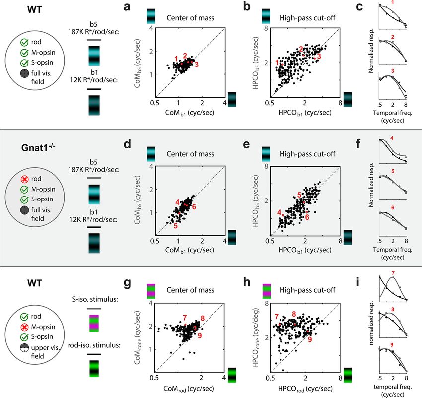
www.nature.com/scientificreports/
function of photoisomerizations(R*)/rod/sec and retinotopic location. First, the model predicts that the dimmest
and brightest settings yield 75% and 5% rod input, relative to cones. The model also gives the balance of cone
M- and S-opsin input as a function vertical retinotopy. Finally, we used the model to predict the state of retinal
adaptation under two hypothetical lighting conditions: a commercial display and outdoor lighting in an urban
setting8. We predict that although a dilated pupil does not allow for rod saturation with a commercial display,
mouse rods quickly saturate at the onset of sunrise. Finally, we isolated cone and rod contrast to characterize their
respective spatio-temporal properties in V1 with 2-photon imaging. We showed that spatial tuning changes little
between rod- and cone-mediated vision. However, cone-mediated V1 encoded substantially higher temporal
frequency than rods.
Results
Measurements of photoreceptor contributions to mouse V1. We imaged anesthetized mouse V1
responses to visual stimuli that were calibrated to modulate distinct photoreceptor opsins across the retina. Two-
photon and widefield calcium imaging of neurons was performed after viral-mediated expression of G CaMP6f9.
Figure 1 outlines features of the mouse preparation and visual stimulus paradigm that were common to all
results from this study. Most recordings were done in wild-type (WT) mice, and a subset of experiments was
repeated in mice lacking rod function ( Gnat1−/−)10. The WT mouse retina has 3 main photoreceptor opsins—
cone M-opsin, cone S-opsin, and rod rhodopsin—which have unique spectral sensitivities functions (Fig. 1a)
and spatial distributions across the retina (Fig. 1b). The upper region of the visual field is filtered primarily
through the S-opsin and rhodopsin sensitivity functions. Conversely, in the lower extreme of the visual field,
images are filtered through the M-opsin and rhodopsin sensitivity functions4, which are very similar.
A major goal of the study was to quantify the balance of input to V1 from all three opsins as a function of
visual field location and light adaptation. To this end, visual stimuli systematically varied along 3 dimensions—
retinotopy, background light level, and color. The vertical retinotopy was mapped at each pixel (widefield imag-
ing) or neuron (2-photon imaging) based on responses to a monochromatic vertical drifting b ar11. The display’s
emitted spectral power (radiance) was nearly constant across the range of viewing angles under study (+ /- 60°),
which allowed for controlled measurements of light adaptation across the retinotopy (Fig. 1d). To alter the state
of light adaptation, the display’s spectral power was scaled to a new midpoint for 10 min, followed by a continu-
ous block of full-field drifting gratings that maintained the same midpoint (Fig. 1e). As will be shown, varying
the state of light adaptation with our display allowed for a wide dynamic range of rod saturation.
Within each block of light adaptation, drifting gratings were shown at variable orientation to generate robust
V1 responses along isolated axes of color space, and/or along a range of spatio-temporal frequencies. Initially,
we show results where spatio-temporal frequency is kept constant and responses are compared between M and S
cone-opsin contrasts (Fig. 1f). These measures of M/S color tuning vs. light adaptation are used to model a) rod
vs. cone inputs to V1 as a function of rod photoisomerization rates, along with b) the retinotopic distribution
of pure cone-opsin inputs to V1. At the end, we use a related paradigm to compare rod-mediated and cone-
mediated spatio-temporal tuning properties in V1.
Revealing the cone mosaic via increasing rod saturation. Here we describe results from the visual
stimulus paradigm introduced above, which varies color and light adaptation. This analysis is limited to experi-
ments with an artificially dilated pupil; subsequent experiments will expand our findings to understand the
impact of an undilated pupil. Since rods are monochromatic and uniformly distributed across the mouse retina,
the entire visual field at night is filtered through a common spectral sensitivity function. However, when the
dichromatic cone population is allowed to take over, there is a gradient of spectral sensitivity along the retina’s
dorsoventral axis that is conveyed to V1 and higher visual areas12. What are the dynamics of the monochromatic-
to-dichromatic photoreceptor transformation at the level of V1 topography, and does our current setup allow
for it to be resolved and thus modeled? To address these questions, we used the experimental paradigm shown
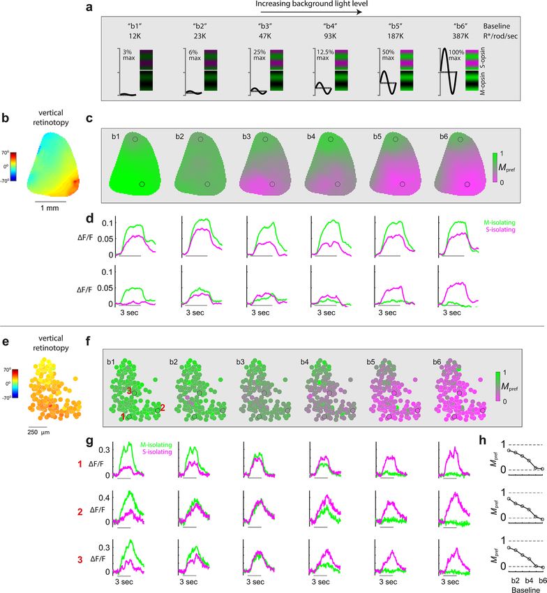
in Fig. 2a; S- and M-isolating gratings of equal contrast were presented after adapting to 6 different light levels.
For each neuron from the 2-photon imaging, and pixel from widefield imaging, we calculated a metric for
color preference, Mpref = FM/(FS + FM), where FM and FS are the mean fluorescence changes in response to the
M- and S-isolating stimuli, respectively. Figure 2 shows the graded unveiling of the Mpref map. At the lowest
light levels, neurons across the entire V1 retinotopy were mostly responsive to M-isolating gratings, indicating
a predominance of rod input. Increasing light levels induced a graded exchange in responsiveness: responses
to M-isolating gratings fell, and responses to S-isolating gratings rose (Fig. 2d,g). In the upper visual field, the
exchange is especially dramatic, as this part of the cone mosaic is dominated by S-opsin—neurons go from
strong preference for the M-opsin gratings (Mpref ~ 1) to strong preference for S-opsin gratings (Mpref ~ 0) with
increasing light level. These examples confirm that the display generates a sufficient range of both intensity and
color to model photoreceptor contributions across the V1 topography.
Modeling opsin contributions to V1 as a function of isomerization rates and visual field loca‑
tion. Next, using the visual stimulus paradigm shown in Fig. 2a, the two-photon data was combined across
animals to model a) the balance of rod and cone inputs as a function of light level and b) the balance of S vs. M
cone-opsin inputs as a function of retinotopy.
Model description. Here, we summarize key elements of the model used to quantify photoreceptor contribu-
tions to V1. The equations given in the Methods describe the response of a V1 neuron to each chromatic grating
(S and M-opsin isolating ) as a linear combination of 3 inputs: rods, S-opsin, and M-opsin. The magnitude of
rod inputs depends only on light levels (not retinotopy), whereas the magnitude of S and M cone opsin inputs
Scientific Reports | (2021) 11:11937 | https://doi.org/10.1038/s41598-021-90650-4 2
Vol:.(1234567890)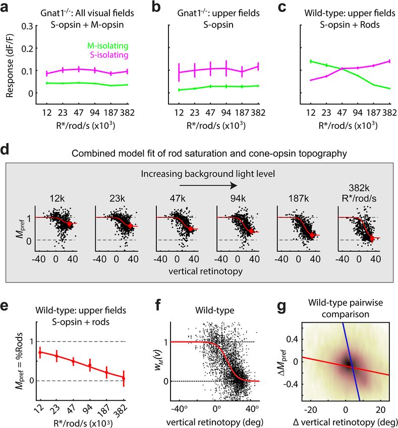
www.nature.com/scientificreports/
Figure 1. Imaging and visual stimuli setup for mapping retinotopy and color in the mouse V1. (a) Opsin
sensitivity functions for 3 different types of opsins found in rod and cone photoreceptors. Rhodopsin peaks at
498 nm, while cone S-opsin and M-opsin peak at 360 nm and 508 nm, respectively. 2 mouse genotypes were
used: wild-type and Gnat1−/−, which is a rod-deficient transgenic strain. (b) Illustration of cone S/M-opsin
expression gradient in mouse retina (left) versus rhodopsin expression (right). Ventral retina (upper visual field)
expresses predominantly S-opsin while dorsal retina (lower visual field) expresses predominantly M-opsin.
Rods are uniformly expressed throughout retina. (c) Rear projection of visual stimuli using two monochromatic
projectors, near-UV (nUV) and green. Screen color depicts corresponding S/M-opsin expression in mouse’s
retina. (d) Measures of the display’s spectral radiance at three viewing angles. Uniformity is required for
controlled light adaptation across the retinotopy. Below are the stimuli used to map retinotopy. (e) A total of 6
background light levels were used to adapt the retina, with each level scaling the spectral radiance by a factor
of 2. Below is an illustration of the adaptation paradigm. Prior to a block of test trials with drifting gratings,
the retina was adapted for 10 min by the midpoint (i.e. “gray level”) of the test trials. (f) Drifting gratings were
calibrated to oscillate along one of three axes in S and M cone-opsin space: S, M, and S + M. The sine-wave insets
indicate relative green and nUV LED amplitude and phase used for each of the three color axes. Below is an
illustration of a stimulus paradigm for measuring color preference, where each trial showed a different color at a
given adaptation level.
depends only on location along the vertical retinotopy (not light level). One assumption with this model is that
rod inputs are uniform across the visual field in an animal that lacks a fovea7. A second assumption is that cone
responses maintain Weber adaptation, meaning that responses depend on contrast and not the range of back-
ground light levels used in this study. We tested this latter assumption, given the proximity of our lowest light
level to cone thresholds (i.e. their “dark light”) established in prior s tudies13,14.
To test for Weber adaptation in cones, we measured V1 responses as a function of light level in mice with
dysfunctional rods (Gnat1−/−)10, which showed that they do not increase with light level, for either S or M-opsin
gratings (Fig. 3a). Figure 3a uses cells at all locations of the retinotopy, whereas Fig. 3b limits the population to
neurons with receptive fields in the upper region of the visual field (> 30° above midline). In both cases, responses
do not change significantly with light level (p > 0.05; Pearson correlation). Figure 3b also shows that neurons in
the upper visual field have near zero response to the M-opsin gratings, as expected. The assumption of Weber
Scientific Reports | (2021) 11:11937 | https://doi.org/10.1038/s41598-021-90650-4 3
Vol.:(0123456789)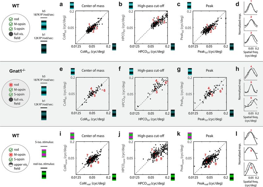
www.nature.com/scientificreports/

                                            Figure 2.  Revealing the cone mosaic’s M-to-S gradient in V1 via progressive rod saturation. (a) Illustration of
                                            the stimuli used to measure color tuning across 6 states of background light adaptation, “b1-b6”. Each subsequent
                                            adaptation levels have mean gray values that differ by a factor of 2, and constant sinewave contrast, depicted on left
                                            side of each subpanel. Prior to each level, the eye was adapted at the same gray value for 10 min. Each trial within a
                                            level block had either a S-opsin or M-opsin isolating grating, depicted on right side of each subpanel. (b–d) Wide-
                                            field calcium imaging. (b) Map of V1’s vertical retinotopy. (c) Maps of Mpref, at each of the 6 states of light adaptation.
                                            Mpref at each pixel indicates the preference for the M-opsin color axis, over the S-opsin color axis. At low light levels,
                                            Mpref ~ 1 at all pixels, indicating rod input—rod inputs are uniform and have nearly identical spectral sensitivity as
                                            M-ospin. At higher light levels, rods saturate, revealing the M-to-S cone opsin gradient. (d) Two rows show time
                                            courses of fluorescence signal at the 2 ROI’s indicated in the map. Top circle corresponds to lower visual field; bottom
                                            circle corresponds to upper visual field. Green and violet traces are responses to M-opsin and S-opsin gratings,
                                            respectively. The line under each pair of traces indicates the stimulus duration. (e–h) 2-photon calcium imaging. (e) V1
                                            map of vertical retinotopy, where each circle is the location of an example neuron. (f) Maps of Mpref, at 6 states of light
                                            adaptation. (g) Each row of time courses is from a different neuron in the ROI (see their locations in Mpref map at left).
                                            Green and violet traces are responses to M-opsin and S-opsin gratings, respectively. (h) Right-most column shows each
                                            example neuron’s mean Mpref during stimulus presentation, as a function of light level.

          Scientific Reports |   (2021) 11:11937 |                https://doi.org/10.1038/s41598-021-90650-4                                                         4

Vol:.(1234567890)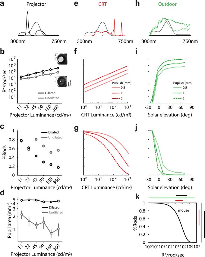
www.nature.com/scientificreports/
Figure 3. Modeling photoreceptor inputs as a function of light adaptation and vertical retinotopy. (a) Mean and
standard error responses of V1 neurons in Gnat1−/− mice, at 6 light levels. This was used to confirm that cones
are in a constant state of Weber adaptation across the range of light levels. (b) The same analysis was performed
as in ‘a’ using a subset of the data, upper visual field neurons (> 30°), which limits the cone inputs to S-opsin. (c)
Mean and standard error responses of V1 neurons in WT mice, at 6 light levels. Data was limited to the upper
visual field to highlight the population’s “switch” in responsiveness from rod- to cone-mediated inputs. (d) The
six panels of Mpref vs. vertical retinotopy show data points from the same WT population, at the six states of light
adaptation. Overlayed in red line is the model fit of Mpref as a function of vertical retinotopy and light adaptation
(see “Methods”). Red dots indicate population average for neurons in the upper visual field of WT mice, which
are shown again in ’e’. (e) The color-tuning metric, “Mpref”, when limited to neurons in the upper visual field of
WT mice, is effectively a measure of the balance of rod vs. cone input, “%Rods”. The mean and standard error
bars of %Rods are shown as a function of light adaptation, and the line shows the model fit. (f) The y-axis,
“wm(v)”, is an estimate of the balance of M- and S- cone opsin providing input to V1 at each retinotopic location.
1 and 0 indicate 100% M- and S-opsin, respectively. Data points are an accumulation from all the panels in
‘d’, after normalizing by the model fit along the dimension of light intensity using the %Rod model in ‘e’. The
red line is the model fit of the retina’s cone opsin gradient (M vs. S cone-opsin input) vs. vertical retinotopy,
recapitulated in V1. (g) Population pairwise comparison of ∆Mpref as a function of ∆vertical retinotopy (r = -0.21;
p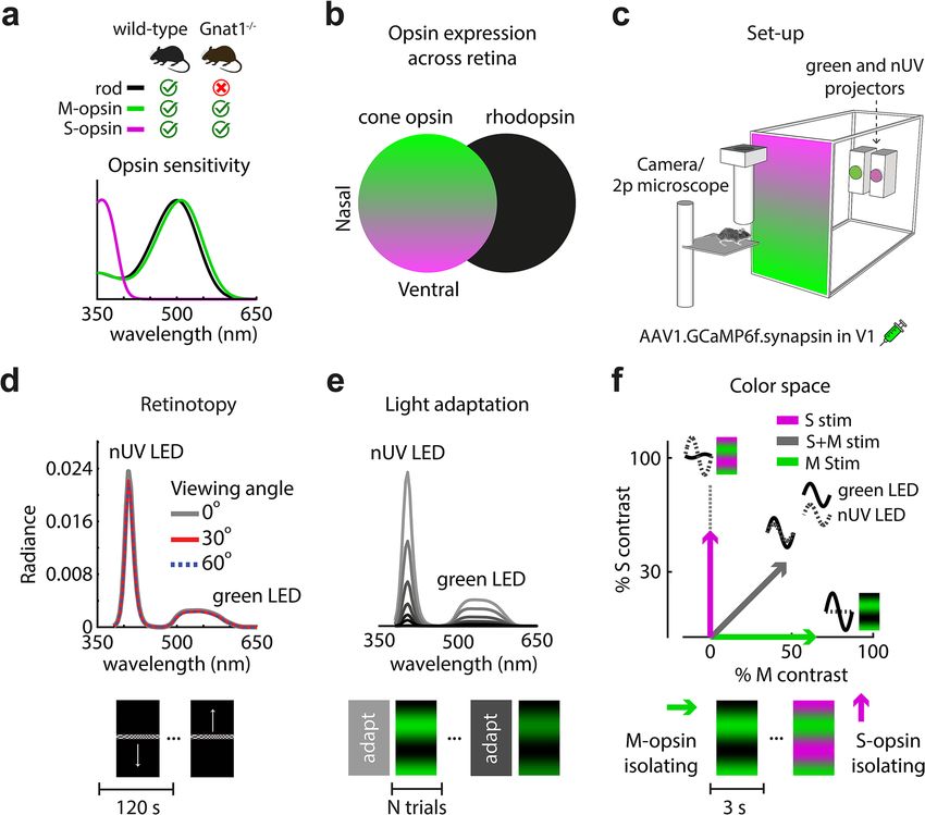
www.nature.com/scientificreports/
adaptation for cones simplified the model, yet accounts for a wide range of lighting conditions. In the Methods,
we derive the model in Eq. 5 below, which expresses the measurement of color tuning, Mpref, as a function of
the input from each opsin, at each retinotopic location and backround light level.
ws (v)ss
Mpref (b, v) = 1 − Model of color tuning response (5)
ss + wr (b)rm
The two functions we solved for are wr (b) and ws (v).wr (b) is the unitless weight of rod input as a function
of background light level. ws (v) is the unitless weight of S-opsin input as a function of vertical retinotopy. The
corresponding weight of M-opsin input is wm (v) = 1 − ws (v). ss is the S-opsin contrast of S-opsin gratings (~ 0.6),
and rm is the rod contrast of the M-opsin gratings (~ 0.6). Under complete rod saturation, wr (b) approaches zero,
giving Mpref (b, v) ∼ 1 − ws (v) = wm (v), which is the pure cone opsin retinotopic gradient. Oppositely, under
low light levels, ws (v) ≪ wr (b), giving Mpref (b, v) ∼ 1, which is pure rod input that only responds to the M-opsin
gratings across the entire V1 topography. Below, we describe the results of fitting ws (v) and wr (b), based on the
measurements of Mpref (b, v).
Model fit of rod saturation. To fit the model to data, we used two-photon responses from 11 WT mice. Fig-
ure 3d plots Mpref against vertical retinotopy, at all 6 light levels. The population shows graded rod saturation
and the emerging cone mosaic with increasing light levels—i.e. from left-to-right, Mpref is reduced and becomes
more steeply correlated with the retinotopy. To simplify the relationship between rod saturation and Mpref,
we limited the data to the subpopulation of neurons that represent the upper visual field (> 30°), which limits
the photoreceptor opsin input to cone S-opsin and rods. Studies in the mouse retina show that cone signals
in the upper visual field are almost exclusively mediated by S-opsin4,15—i.e. ws (v > 30) = 1, where 30° is a
conservative threshold based on these prior studies. By limiting responses to the upper field, it can be shown
that the measured color preference, Mpref , is equal to the proportion of rod input, relative to cones, defined as
%Rod(b) = wr (b)/[wr (b) + ws (v > 30)]. In turn,
0.586
the y-axis of Fig. 3e is shown as “ Mpref = % Rod”. The trend of
% Rod(b) is well-fit by the equation e−0.072(b) . The data shows that the minimum and maximum light level
of the display (b1 and b6) yield rod contributions to V1 of 75% (%Rod = 0.75) and 5% (%Rod = 0.05), relative to
the cones.
Model fit of M‑to‑S cone opsin topography in V1. In a previous study, we showed that the M-to-S cone opsin
gradient is recapitulated in V1 and higher visual areas12. However, this prior study did not account for potential
rod “contamination” in measuring the cone opsin map, and it employed intrinsic signal imaging. Here, we were
able to remove the rod contamination using the model of %Rod(b) in Fig. 3e. The topographic map of cone
[1−Mpref ]
opsin inputs to V1, wm (v) = 1 − ws (v), is dependent on known variables in our model: wm (v) = 1 − [1−%Rod] .
Specifically, this equation converts the measured values of color preference, Mpref (b, v) (Fig. 3d, all panels), into
the cone-opsin topographic map, wm (v) (Fig. 3f, black points), by way of the model fit to %Rod(b) (Fig. 3e).
The fitted red curve in Fig. 3f is ŵm (v) = 1+e0.192(v−14)
1
. Finally, ŵm (v) was converted to M̂pref (b, v), by way of the
model fit to %Rod(b), and overlaid on the data points in Fig. 3d (red).
Pairwise comparison of M pref against retinotopy in V1. Thus far, we’ve shown a clear relationship between the
vertical retinotopy and color preference. To further quantify the cell-by-cell continuity of the maps, we compared
the pairwise change in retinotopy to the pairwise change in Mpref . Baseline 5 in the WT population was used for
this analysis (Fig. 3d, 187 k R*/rod/sec). For every pair of data points within each ROI (> 38 K pairs), we calcu-
lated the change in Mpref and in vertical retinotopy, which yielded the density plot in Fig. 3g. There is a signifi-
cant correlation (r = − 0.21; p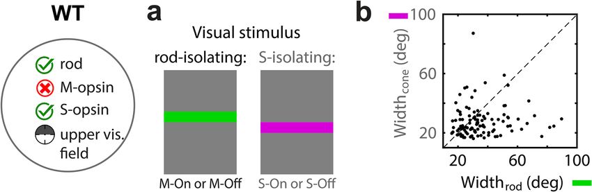
www.nature.com/scientificreports/

                                  Figure 4.  Variable states of retinal adaptation via pupil size, background light level, and stimulus source. (a) In black
                                  is the spectrum of the projector used in this study, with both green and nUV LEDs ‘”on”. (b) Rod isomerization rates
                                  measured at variable projector background light level, with and without application of tropicamide. To begin, the 6
                                  adaptation blocks were shown, in ascending order (b1-to-b6), to an undilated (naive) pupil. Next, the pupil was dilated
                                  using tropicamide and reshown the 6 stimulus adaptation blocks in descending order (b6-to-b1). (c) %Rod input to
                                  V1 as a function of projector luminance values, for undilated and dilated pupils. (d) Mean and standard error of pupil
                                  area at 6 light levels (x-axis) with and without application of tropicamide. (e) In red is the spectral power distribution
                                  of a CRT with RGB guns all “on”. (f) Model of mouse rod isomerization rates over a wide range of CRT intensity, in cd/
                                  m2. (g) Prediction of %Rod contribution to V1 as a function of CRT luminance values. (h) In solid green is the power
                                  distribution of the CIE D65 standard, used as the daylight spectrum. The dashed green line is the spectrum used after
                                  sunset. Absolute daylight irradiance values were obtained from Spitschan et al.8 (i) Model of rod isomerization rates
                                  at varying solar elevation in an urban setting. (j) Prediction of %Rod contribution as a function of solar elevation.
                                  Positive and negative is above and below the horizon, respectively. (k) In black is the model fit of %Rod contribution
                                  vs. rod isomerization rates. It was used to transform the plots in ‘f ’ and ‘i’ into the plots in ‘g’ and ‘j’. The color bars on
                                  top approximate the range of rod isomerization rates generated by each stimulus source. Similarly, the y-axis shows the
                                  ability of each source to push the rodent retina into a photopic (i.e. %Rod = 0) vs. scotopic (i.e. %Rod = 1) state.

Scientific Reports |   (2021) 11:11937 |                 https://doi.org/10.1038/s41598-021-90650-4                                                              7

                                                                                                                                                           Vol.:(0123456789)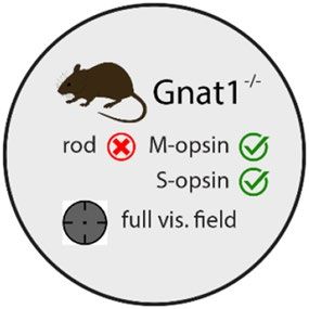
www.nature.com/scientificreports/
same time, luminance ignores the spectral power produced by the nUV LED in our set-up, which will also help
saturate mouse rods. Specifically, the green LED and nUV LED account for 63% and 37% of the rod isomerizing
power in the display based on their overlap with the rhodopsin sensitivity function, respectively.
%Rod inputs to mouse V1 when exposed to outdoor lighting and commercial displays. In
Fig. 3e, we used responses to variable light intensity to fit a model of the percentage of rod input to V1, relative to
cone input, as a function of rod isomerization rate; viz. %Rod(b). Here, we used this model to make predictions
of %Rod under two other relevant environments. We first asked what %Rod values are achieved under “stand-
ard” luminance (cd/m2) intensity produced by a commercial display. We show that these standard luminance
levels yield mostly rod input. We then asked if the mouse retina can achieve a photopic state when exposed to
natural outdoor lighting, and if so, what time of day the transition occurs.
Commercial displays do not drive cone S-opsin, but do drive rods and cone M-opsin. To make predictions of
rod saturation relative to M-opsin inputs (i.e. %Rods) when exposed to a commercial display, we made radiomet-
ric measurements of a CRT monitor. The CRT results can be expected to generalize to other commercial displays
since spectral irradiance profiles of ‘blue’ and ‘green’ will be quite similar (‘red’ may be unique in a CRT, but
has minimal overlap with mouse photoreceptors). The CRT’s spectral radiance was compared to rod sensitivity
functions (Fig. 4e) to calculate R*/rod/s as a function of CRT luminance (Fig. 4f). Then, each value of R*/rod/s
was inserted into the model fit in Fig. 4k (previously shown with data in Fig. 3e) to yield the fraction of rod input,
%Rods. Together, this gave curves of %Rods vs. luminance (Fig. 4g), which is a more relatable domain in most
areas of vision science. A typical display produces luminance around 1 02 cd/m2. At 1 02 cd/m2, Fig. 4g shows that
V1 is mostly rod-mediated unless the pupil is fully dilated. This differs from the primate in that 1 02 cd/m2 is
expected to put the retina into a photopic regime. Finally, we reiterate that these CRT predictions only pertain to
M-opsin in the cone mosaic, which are expressed only in the dorsal half of the retina. The spectral power from
commercial displays does not overlap with the spectral sensitivity function of S-opsin, so the cone mosaic will
remain silent in the ventral half of the retina, regardless of background intensity.
If commercial displays cannot yield a cone-mediated mouse V1, a natural follow-up question is whether day-
light can produce cone-mediated V1. For this, we used spectral irradiance measurements (Watts/µm2retina /� )
at variable solar elevation taken in a recent study (Fig. 4h, green)8. Combined with the rod sensitivity function,
the solar spectral irradiance measurements gave R*/rod/sec vs. solar elevation (Fig. 4i). Finally, we plugged R*/
rod/sec into our model fit (Fig. 4k) to give %Rod vs. solar elevation (Fig. 4j). Unlike a commercial display, solar
radiation has power at wavelengths to drive both M and S opsin. The curves show that the mouse retina rapidly
approaches a photopic state after sunrise. Figure 4k provides a summary comparison of the dynamic range of
light adaptation in the mouse retina for three lighting conditions. Natural outdoor lighting (green line) spans
the full range, from scotopic to photopic. Both of the two experimental displays examined—our projector set-up
and commercial displays—place the retina in the mesopic transition zone. However, the relatively incremental
advantage provided by the nUV power and overall brightness in our projector system (Fig. 4k; compare blue and
red, on top) is able to push the retina near a photopic state (Fig. 4k; compare blue and red, on right). In summary,
although we have used seemingly extreme experimental condition to approach photopic vision, the difference
from commercial displays is minor relative to the bounds of outdoor lighting.
A final note on interpretation of these results: the model of %Rod vs. rod isomerization rate is independent
of cone adaptation under the assumption that cones are above the dark noise, and into Weber adaptation. It
is for this reason that we only need to consider overlap with the rod sensitivity function to predict %Rod at a
given level of light adaptation. For instance, our nUV LED does not have much overlap with S-opsin sensitivity
(Fig. 1a,d), yet has sufficient power to place the S-cones into Weber adaptation at the lowest light levels studied
(Fig. 3a,b). In the case of the CRT, there is no overlap with S-opsin, so these plotted predictions only pertain to
M-opsin in lower visual fields. In upper fields, the %Rod prediction is 100% with a commercial display.
V1 responds to higher temporal frequencies when stimuli drive cones more than rods. Rods
and cones are routed through different pathways in the retina that filter unique spatio-temporal properties of the
visual scene for further processing in the cortex. To date, studies of detailed spatio-temporal tuning in mouse
V1 are largely rod-mediated, as predicted by the results in Fig. 4. Here, we asked if V1’s spatio-temporal tuning
properties change when we vary %Rods—the balance of rod and cone input. Two methods were used to alter
%Rods—one that varied the state of light adaptation (i.e. rod saturation), and the other that varied color (i.e.
rod and cone contrast). For the light adaptation method, rod-deficient (Gnat1−/−) mice were used as a control.
Temporal frequency tuning was measured under two background light levels, b1 (12 K R*/rod/sec) and b5
(200 K R*/rod/sec), where the predicted %Rod input is 75% (i.e. 25% cones) and 20% (i.e. 80% cones), respec-
tively. Figure 5a-c and Table 1 show that there is a shift in tuning toward higher temporal frequencies when cones
provide the primary input. For each neuron, we used two parameters from Gaussian fits to quantify tuning at
each level of rod saturation, center-of-mass ( CoMb1 & C oMb5) and the high-pass cut-off frequency ( HPCOb1 &
HPCOb5). To quantify differences, we calculated the geometric mean of the ratio between tuning parameters. In
turn, paired t-tests were performed on the logs—e.g. log(CoMb1) vs. log(CoMb5). The geometric mean of C oMb5/
CoMb1 was 1.12 (i.e. 12% change) and was significantly greater than one (p = 2.47e−35). The geometric mean of
HPCOb5/HPCOb1 was 1.38 (p = 1.76e−32). To verify that these results were due to an exchange in activity between
rods and cones, we repeated these experiments and analyses in Gnat1−/− mice (Fig. 5d-f). While the difference
in tuning for spatial or temporal frequencies between the two light levels were statistically significant, there
were nominal difference in calculated means: geometric mean of CoMb5/CoMb1 = 1.00 (p = 0.012); geometric of
HPCOb5/HPCOb1 = 1.01 (p = 0.0047).
Scientific Reports | (2021) 11:11937 | https://doi.org/10.1038/s41598-021-90650-4 8
Vol:.(1234567890)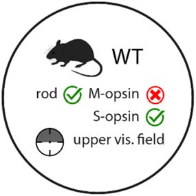
www.nature.com/scientificreports/
Figure 5. V1 responds to higher temporal frequencies when stimuli drive cones more than rods. Top row (‘a-
c’) is data from WT mice, comparing temporal frequency tuning at two light adaptation levels, “b1” and “b5”,
corresponding to 12 K and 187 K R*/rod/sec (n = 235). (a) Scatter plot compares the temporal frequency tuning
curve’s center-of-mass (CoM) at b5 (y-axis) and b1 (x-axis). Unity line is dashed black line. The geometric mean
of CoMb5/CoMb1 is 1.12 (i.e. 12% change; t-test: p = 2.47e−35). (b) Same as in ‘a’, but the temporal frequency
tuning parameter is the high-pass cut-off frequency (HPCO). The geometric mean of H PCOb5/HPCOb1 is
1.38 (t-test: p = 1.76e−32). (c) Tuning and fits of 3 example neurons at the 5th, 50th, and 95th percentile of the
HPCOb5/HPCOb1 distribution from ‘b’. Dots are normalized responses and lines are the fits. In each case, black
and gray correspond to ‘b1’ and ‘b5’, respectively. Next, middle row of panels (‘d-f ’) shows data from rod-
deficient Gnat1−/− mice, using the same experiment and analysis as in the top row (n = 244). (d) The geometric
mean of CoMb5/CoMb1 is 1.00 (t-test: p = 0.012). (e) The geometric mean of HPCOb5/HPCOb1 is 1.01 (t-test:
p = 0.0047). (f) Tuning and fits of 3 example neurons at the 5th, 50th, and 95th percentile of the distribution
of HPCOb5/HPCOb1 from ‘e’. Bottom row of panels (‘g-i’) shows data from WT mice, limited to neurons with
a receptive field 30-deg above the retina’s midline where opsin expression is mostly limited to S-opsin and
rhodopsin (n = 218). Here, background light levels were held constant at b5 and tuning was compared between
stimuli of isolating cone- and rod-contrast. (g) Scatter plot compares temporal frequency tuning CoM between
the rod (x-axis) and cone (y-axis) isolating contrasts. Geometric mean of C oMcone/CoMrod is 1.42 (t-test:
p = 1.91e−31). (h) Same as in ‘g’, but the parameter measurement for each neuron and light level is HPCO.
Geometric mean of HPCOcone/HPCOrod is 2.54 (t-test: p = 1.97e−51). (i) Tuning and fits of 3 example neurons at
the 5th, 50th, and 95th percentile of the distribution of HPCOcone/HPCOrod.
Scientific Reports | (2021) 11:11937 | https://doi.org/10.1038/s41598-021-90650-4 9
Vol.:(0123456789)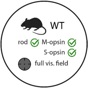
www.nature.com/scientificreports/
b1: 1.19 (± .17) b1: 1.30 (± .66) Rod: 1.32 (± .31)
Center-of-mass
b5: 1.33 (± .13)*** b5: 1.31 (± .81)* S-opsin: 1.86 (± .24)***
Temporal frequency (cyc/s)
b1: 1.38 (± .88) b1: 1.95 (± 1.36) Rod: 1.15 (± .68)
High-pass cutoff
b5: 1.91 (± .84)*** b5: 1.90 (± 1.35)** S-opsin: 2.92 (± .88)***
b1: 0.05 (± .01) b1: 0.050 (± .02) Rod: 0.046 (± .018)
Center-of-mass
b5: 0.05 (± .013)*** b5: 0.053 (± .018)* S-opsin: 0.047 (± .013)***
b1: 0.084 (± .036) b1: 0.085 (± .046) Rod: 0.080 (± .038)
Spatial frequency (cyc/deg) High-pass cutoff
b5: 0.076 (± .022)*** b5: 0.090 (± .041)* S-opsin: 0.073 (± .026)***
b1: 0.047 (± .024) b1: 0.050 (± .033) Rod: 0.043 (± .025)
Peak
b5: 0.045 (± .014)*** b5: 0.053 (± .028)* S-opsin: 0.040 (± .018)**
— — Rod: 35.62 (± 15.51)
Receptive field size (deg) Width
— — S-opsin: 27.74 (± 10.59)***
Table 1. Summary of spatio-temporal tuning estimates, outlining parameter mean and standard deviation
values from Figs. 5, 6 and 7. Parameter estimates for temporal frequency, spatial frequency, and receptive
field size mapping experiments from Figs. 5, 6 and 7, respectively, compiled in table format. First 2 rows
outline temporal frequency curve fit parameter estimates of center-of-mass and high-pass cutoff for “b1”
(12 K R*/rod/sec) vs. “b5” (187 K R*/rod/sec) conditions in wild-type mice (3rd column), “b1” vs. “b5” in
rodless (Gnat1−/−) mice (4th column), and “b5” cone vs. rod inputs in wild-type mice (5th column). “Rod”
and “S-opsin” in last (5th) column indicate M-opsin contrast and S-opsin contrast stimuli used, respectively.
Next 3 rows outline spatial frequency curve fit parameter estimates of center-of-mass, high-pass cutoff, and
peak for “b1” vs. “b5” conditions in wild-type mice (3rd column), “b1” vs. “b5” but in rodless ( Gnat1−/−) mice
(4th column), and “b5” cone vs. rod inputs in wild-type mice (5th column). Last row outlines receptive field
size comparison, measured as 2σ of Gaussian fit, between “b5” rod vs. cone inputs in wild-type mice. For
each measurement listed, “mu (± std)” format is used to denote geometric mean value followed by standard
deviation for temporal-spatial frequency parameters. “mu (± std)” format is used to denote arithmetic mean
value followed by standard deviation for receptive field size estimates. “*/**/***” state statistical significance of
p-values under .05, .01, and .001, respectively.
Next, we used a different method to compare temporal frequency tuning between rod and cone-mediated
inputs. This method kept the light adaptation at a constant mesopic level, but varied rod and cone contrast. Just
as in previously described experiments (Figs. 2, 3, 4), stimuli had color contrast that isolate either S-opsin or
M-opsin (Fig. 1f). However, here the analysis was limited to neurons with upper receptive fields (> 30° above
midline), so the M-opsin stimulus is effectively a rod-isolating stimulus; i.e. M-opsin and rods have nearly identi-
cal spectral sensitivity, yet the upper fields lack M-opsin. For the same reason, the S-opsin stimulus is effectively a
cone-isolating stimulus (more specifically, the calculated rod contrast is 2% in response to the S-opsin stimulus).
Figure 5g-i shows the comparison of temporal frequency tuning between the two different color directions. The
results are consistent with the changes induced by different light adaptation levels in Fig. 5a-c, in that the cone-
dominated tuning is shifted to higher values of temporal frequency. However, the differences are stronger with the
method of rod- and cone-isolating contrasts, which may be attributed to purer separation of rod and cone drive.
The geometric mean of C oMcone/CoMrod is 1.42 (i.e. 42% change), and significantly greater than 1 (p = 1.91e−31).
The geometric mean of HPCOcone/HPCOrod exhibited the strongest differential, at 2.54 (p = 1.97e−51).
Many neurons in mouse V1 are highly selective for orientation. However, the results above used temporal
frequency tuning curves from the average over orientation, as this gave the highest data yield using the criteria
described in the methods. Averaging over orientation reduces the “signal”, but also reduces the “noise”. None-
theless, this leaves open the possibility that results could differ when only the peak orientation is used. We thus
repeated the analysis described immediately above (viz. for Fig. 5g-i), but only used the peak orientation to
calculate temporal frequency tuning. Results were consistent, although the differential of HPCO was lower.
The geometric mean of CoMcone/CoMrod is 1.41, and significantly greater than 1 (p = 3.28e−5). The geometric
mean of HPCOcone/HPCOrod was 1.83 (p = 0.0012). Cell yield dropped to 68% of the original analysis method
of averaging over orientation.
Cone‑ and rod‑mediated V1 responds to a similar band of spatial frequencies. Similar analyses
were performed for spatial frequency tuning as those described above for temporal frequency tuning. Three
parameters were taken from Gaussian fits to the spatial frequency tuning curves: peak location, CoM, and HPCO.
The comparisons between two levels rod saturation (b1 and b5) in WT mice are shown in Fig. 6a-d and Table 1.
The tuning is quite similar between the two states of adaptation. However, there is a small but significant shift in
tuning to lower spatial frequencies when cones are the primary input: Geometric mean of Peakb5/Peakb1 = 0.94
(p = 2.07e−7), CoMb5/CoMb1 = 0.96 (p = 1.04−6), and HPCOb5/HPCOb1 = 0.90 (p = 2.4e−17). For Gnat1−/− mice, this
Scientific Reports | (2021) 11:11937 | https://doi.org/10.1038/s41598-021-90650-4 10
Vol:.(1234567890)www.nature.com/scientificreports/
Figure 6. Rod-driven responses in V1 have marginally higher spatial frequency tuning than cone-driven
responses. Top row (‘a-d’) shows data from WT mice, comparing spatial frequency tuning at two light
adaptation levels, “b1” and “b5”, corresponding to 12 K and 187 K R*/rod/sec (n = 250). (a) Scatter plot
compares center-of-mass (CoM) estimates of spatial frequency tuning curve at b5 (y-axis) and b1 (x-axis). Each
data point represents a single neuron. Unity line is dashed black line. The geometric mean of C oMb5/CoMb1 is
0.96 (t-test: p = 1.04e−6). (b) Same as in ‘a’ but the spatial frequency tuning parameter is the high-pass cut-off
frequency (HPCO). The geometric mean of H PCOb5/HPCOb1 is 0.90 (t-test: p = 2.40e−17). (c) Same as in ‘a,b’ but
the spatial frequency tuning parameter is the peak spatial frequency (“Peak”). The geometric mean of P eakb5/
Peakb1 is 0.94 (t-test: p = 2.07e−7). (d) Tuning and fits of 3 example neurons at the 5th, 50th, and 95th percentile
of the distribution of HPCOb5/HPCOb1. Dots are normalized responses and lines are the fits. In each case, black
and gray correspond to ‘b1’ and ‘b5’, respectively. Next, middle row of panels (‘e–h’) is data from rod-deficient
Gnat1−/− mice, using the same experiment and analysis as in the top row (n = 72). (e) The geometric mean of
CoMb5/CoMb1 is 1.05 (t-test: p = .013). (f) The geometric mean HPCOb5/HPCOb1 is 1.06 (t-test: p = 0.021). (g)
The geometric mean of Peakb5/Peakb1 is 1.06 (t-test: p = .029). (h) Tuning and fits of 3 example neurons at the
5th, 50th, and 95th percentile of the distribution of HPCOb5/HPCOb1 from ‘f ’. Bottom row of panels (‘i-l’) shows
data from WT mice, limited to neurons with a receptive field 30-deg above the midline where expression is
mostly limited to S-opsin and rhodopsin (n = 361). Here, the background light levels were held constant at b4
or b5 and tuning was compared between stimuli of isolating cone- and rod-contrast. (i) Scatter plot compares
spatial frequency tuning CoM between the rod (x-axis) and cone (y-axis) isolating contrasts. Geometric mean of
CoMcone/CoMrod is 1.02 (t-test: p = 3.35e−4). (j) Same as in ‘i’ but for HPCO. The geometric mean of HPCOcone/
HPCOrod is 0.91 (t-test: p = 1.79e−4). (k) Same as in ‘i’ but for Peak. The geometric mean of P eakcone/Peakrod is
0.93 (t-test: p = 4.69e−3). (l) Spatial frequency tuning and fits of 3 example neurons at the 5th, 50th, and 95th
percentile of the distribution of HPCOcone/HPCOrod.
analysis also revealed a significant but minute difference in tuning for all of the three parameters. However, in
this case, the higher light levels yielded tuning for higher spatial frequencies (Fig. 6e-h, Table 1).
Then, at a mesopic light level, we compared spatial frequency tuning between cone and rod stimuli in the
upper visual field (> 30° above midline) (Fig. 6i-l). Similar to the results above with rod saturation, there was not
much visually discernable difference in tuning across the two sets of gratings However, there was a statistically
significant difference whereby rod mediated V1 responded to higher spatial frequencies. The main findings of
the spatio-temporal tuning comparison between rod and cone inputs are summarized in Table 1.
Next, we repeated the analysis described immediately above (viz. for Fig. 6i-l), but calculated spatial fre-
quency tuning at a single preferred orientation instead of averaging over all orientations. Results were consistent:
Scientific Reports | (2021) 11:11937 | https://doi.org/10.1038/s41598-021-90650-4 11
Vol.:(0123456789)www.nature.com/scientificreports/
Figure 7. Rod-mediated V1 has larger receptive fields than cone-mediated V1. (a) Horizontal bars (6° in
vertical width, at 2.8° intervals) were intermittently flashed on the screen, varying in color (M-ON, M-OFF,
S-ON, or S-OFF) on constant background light level of ‘b5’ (187 K R*/rod/sec). Data is shown for WT mice,
limited to neurons with a receptive field 30-deg above the midline where expression is mostly limited to S-opsin
and rhodopsin (n = 108). A Gaussian curve is fit to each neuron’s tuning curve of response vs. bar position, for
Rod and S-opsin contrast, which was used to compare receptive field size. Rod isolating contrasts combine
responses from both M-ON and M-OFF bars. Cone isolating contrasts combine responses from both S-ON and
S-OFF bars. (b) Scatter plot compares receptive field width (2σ) between rod (x-axis) and cone (y-axis) isolating
contrasts. Each data point represents a single neuron. Unity line is dashed black line. The mean difference is 7.9
visual angle degrees; geometric mean of Widthcone/Widthrod = 0.83 (t-test: 5.04e−4).
Geometric mean of Peakcone/Peakrod = 1.01 (p = 1.19e−4), CoMcone/CoMrod = 0.99 (p = 0.0026), and HPCOcone/HPC-
Orod = 0.93 (p = 0.0043). Similar to the temporal frequency analysis, when the data was reanalyzed using only the
peak orientation, cell yield dropped to 42% of the original analysis method.
V1 has narrower receptive fields when stimuli drive cones more than rods. To further character-
ize rod vs. cone-mediated differences in V1’s spatial tuning, receptive field width was measured along the verti-
cal dimension of the visual field. The contrast of horizontal bars against a mesopic background was along either
the S- or M-axis of color space. As described above (Figs. 5g-i and 6i-l), under mesopic adaptation in the upper
visual field, the S- and M-opsin stimuli isolate cones and rods, respectively.
This yielded two spatial tuning curves for each neuron, to which the σ of Gaussian fits quantified the recep-
tive field width under cone- and rod-mediated inputs (Fig. 7; Table 1). The mean receptive field width (2σ) for
rod- and cone-mediated inputs was, 35.6° and 27.7°, respectively. The mean of the difference, W idthrod–Widthcone,
was 7.9°. The geometric mean of their ratio, W idthcone/Widthrod, was 0.83 (p = 5.04e−4; t-test). In summary, V1
receptive fields are wider when rod-mediated.
Discussion
The visual stimuli needed to drive cones in and around the fovea is well understood in the primate, which has
guided the engineering of commercial displays that drive the perceptual gamut of trichromatic primate vision.
The mouse retina, while exhibiting many similarities in structure and function to the primate, lacks a fovea and
contains UV-sensitive cone-opsin. Furthermore, the geometry and optical properties of the mouse’s eye produce
retinal irradiance for a given stimulus that will be different than in the primate eye18. Overall, the balance of inputs
from rods and cones to the rest of the mouse’s visual system is difficult to extrapolate from primate psychophysics
and rodent recordings in the retina. Here, we used a simple measure of color tuning to model the balance of rod
and cone inputs to mouse V1, as a function of background light levels. With this model in-hand, we simulated
the balance of rod and cone input to V1 when the eye is exposed to other relevant environments—sunrise puts
the mouse retina into a photopic regime, whereas a commercial display does not. Finally, we used our calibra-
tion of photoreceptor inputs to design experiments that test the differential contributions of rods and cones
to spatio-temporal tuning in V1. Using two different experimental methods, we show a significant increase in
responsiveness to higher temporal frequencies in the transition from rod- to cone-mediated vision. We then
used the same methods to show that cone-mediated vision produces narrower receptive fields, yet comparable
spatial frequency tuning.
Photoreceptor drive with commercial displays in prior studies of mouse visual cortex. Prior
studies of the mouse visual cortex have largely ignored the photoreceptor classes being driven. Nevertheless,
one can assume that visible wavelengths in the upper visual field produce rod-mediated responses. In the lower
visual fields, the cones express green-sensitive M-opsin, and thus are capable of being driven by commercial
displays. However, the simulation in Fig. 4g shows that the luminance values required to saturate the rods and
achieve M-opsin mediated vision are outside the range of commercial displays, even with a fully dilated pupil.
An additional factor to consider with commercial displays is their attenuation of intensity with increasing
viewing angle. This is an issue when imaging mouse visual cortex since a wider range of viewing angles is required
to drive all the recorded cells across the retinotopy. Specifically, our simulation of %Rod for a commercial display
(Fig. 4g) is expected to yield even higher values at the edges of common displays, assuming calibrations were
Scientific Reports | (2021) 11:11937 | https://doi.org/10.1038/s41598-021-90650-4 12
Vol:.(1234567890)www.nature.com/scientificreports/
made orthogonal to the screen. To quantify this, we made spectral radiance measurement of an LCD panel at vari-
able viewing angle. It was found that peak radiance off the LCD panel was attenuated by 45% and 95% at 30° and
60° viewing angles, relative to the max at 0° viewing angle. As shown in Fig. 1d, the rear projection display used
in this study is Lambertian—the spectral radiance does not change with viewing angle. In turn, our simulations
on the required luminance to saturate rods with a commercial display (Fig. 4g) are effectively underestimating
rod saturation at most screen positions.
Taken together, we believe that virtually all prior recordings in mouse visual cortex should be interpreted as
rod-mediated, particularly those where a commercial display was used. As we show here, prior results on spatial
frequency tuning may be expected to generalize to other light adaptation regimes, yet receptive field size and
temporal frequency tuning are not. Even when UV light sources were used with non-commercial displays in prior
studies, our data in Figs. 3e,4c shows that rod saturation is still quite unlikely. This would explain why a transition
from green-to-UV selectivity, with increasing light intensity (e.g. as we show in Figs. 2 and 3), was not observed
in19. Furthermore, studies that utilize combinations of UV and visible stimuli to assess downstream maps of
S- and M-opsin selectivity are likely including rod input, thus obscuring the topographic S-to-M g radient 20,21.
The required light levels to reach cone‑mediated responses can vary. The light intensity
required to saturate rods has been measured at varying stages along the rodent visual pathway, and via medley
techniques4,13,22–24, placing it somewhere between 103 and 1 05 R*/rod/sec. Although several factors are likely to
contribute to this variability, a recent and notable study showed that a critical variable is the length of adaptation
time25. After 10 min of exposure to 1 05 R*/rod/sec, an intensity generally presumed to saturate rods, they showed
that ~ 50% of ganglion cells regain their responsiveness. Our brightest light levels resulted in cone-mediated
responses following a 10 min adaptation window, which may seem contradictory to these reported temporal
dynamics of rod recovery. However, there are two distinctions worth noting.
First, our brightest light levels are just above 1 05 R*/rod/sec, where rod saturation appears to be more
sustainable4,25,26. Second, we calculated the balance of rods vs. cones (%Rods), not absolute rod saturation.
Residual rod signals may indeed remain at our brightest adaptation point (‘b6’), yet are very small relative to the
cones. Furthermore, accumulated noise at the level of cortex precludes the detection of smaller signals in the
retina. Finally, there is the question of rod recovery dynamics at the lower light levels in our adaptation paradigm
(b1–b5). These were played out in descending order following the brightest background condition (b6), and thus
expected to be in a steadier regime of rod recovery’s temporal dynamics25.
Differences in rod saturation across studies may be further accounted for by two related experimental vari-
ables: 1) presence or absence of rod-cone interactions in the retina, and 2) recording location along the retinotopy.
The overlapping spectral sensitivities of rods and cones makes it challenging to drive them independently. For
this reason, studies have used mouse lines that lack functional cones. However, mice lacking cone function to
ouse27,28. Furthermore, more
assess rod saturation will not be subject to the substantial cone-rod crosstalk in the m
recent studies have shown that photoreceptor distributions and retinal circuits are more demarcated along the
dorsoventral axis than originally thought29–31. As a result, rod-cone interactions may also affect rod saturation
in mice with normal retinas, in a retinotopic-dependent fashion.
Rod‑ vs. cone‑mediated temporal receptive field properties in mouse visual cortex. Cone-
mediated temporal dynamics in the retina are much faster than rods, and retinal ganglion cells respond to higher
temporal frequencies when inputs originate from cones4. Therefore, a cone-induced tuning shift toward higher
temporal frequencies by most V1 neurons (Fig. 5) is expected based on inheritance from responses at the output
of the retina. However, the magnitude of the tuning shift in V1 cannot be directly inferred from retinal studies,
as the cortex is known to attenuate higher temporal frequencies—there is low-pass filtering at the first synapse
from LGN inputs32, but also between layer 4 and our recording location, layer 2/333. This is consistent with the
fact that the shift we observed in V1 is not quite as dramatic as what was observed in retinal ganglion cells by
Wang et al.4 Another factor that may have influenced temporal frequency tuning in our preparation was anes-
thesia. V1 response dynamics in awake mice have much more rapid dynamics than anesthetized mice 34, which
may translate to greater responsiveness to higher temporal frequencies. Therefore, the cortical attenuation of
rapid LGN dynamics may be alleviated in the awake prep, thus leading to a more dramatic shift to high temporal
frequencies with cone-mediated vision than what has been observed in Fig. 5.
Rod‑ vs. cone‑mediated spatial receptive field properties in a rod dominated retina. We
observed a 20% reduction in the size of V1 receptive fields (RFs) at photopic light levels, which may be attrib-
uted to inheritance of RF size adaptations in the retina. However, support is lacking for modulations of retinal
ganglion cell (RGC) RF size. More specifically, studies report the absence of a systematic change in the size of
the center-component of RGC RFs, albeit a partial disappearance of the surround in scotopic conditions35–37.
Furthermore, if V1 were to inherit size-adaptions from the retina, one could expect a corresponding adaptation
in SF tuning - viz. a shift toward higher spatial frequencies as RF sizes shrink - but this was not observed in our
data. Instead, spatial frequency tuning was similar across light levels, and even changed subtly in the oppo-
site direction of this model. To offer a descriptive explanation of these observations, we start with a 1D Gabor
model of V1 RFs. If the sinewave frequency remains the same across states of light adaptation, but the Gaussian
envelope widens during scotopic lighting, this would create the observed changes in our data—wider RFs and
a slight shift in tuning toward higher SFs. We can only speculate on a mechanism that mediates a wider Gabor
envelope; e.g. as a widening of cortical pooling from geniculate inputs. Alternatively, cone-mediated vision could
yield relatively unbalanced ON and OFF input to V1 (e.g. due to a sparsely sampled cone mosaic), which would
Scientific Reports | (2021) 11:11937 | https://doi.org/10.1038/s41598-021-90650-4 13
Vol.:(0123456789)You can also read