Geography of a sports metropolis - Gabriel M. Ahlfeldt and Arne Feddersen
←
→
Page content transcription
If your browser does not render page correctly, please read the page content below
Gabriel M. Ahlfeldt and Arne Feddersen
Geography of a sports metropolis

Article (Published version)
(Refereed)

Original citation:

Ahlfeldt, Gabriel M. and Feddersen, Arne (2010) Geography of a sports metropolis. Région et Développement,
31 . ISSN 1267-5059

© 2010 L'Harmattan

This version available at: http://eprints.lse.ac.uk/29080/
Available in LSE Research Online: January 2013

LSE has developed LSE Research Online so that users may access research output of the
School. Copyright © and Moral Rights for the papers on this site are retained by the individual
authors and/or other copyright owners. Users may download and/or print one copy of any
article(s) in LSE Research Online to facilitate their private study or for non-commercial research.
You may not engage in further distribution of the material or use it for any profit-making activities
or any commercial gain. You may freely distribute the URL (http://eprints.lse.ac.uk) of the LSE
Research Online website.
__________________ Région et Développement n° 31-2010 ___________________
GEOGRAPHY OF A SPORTS METROPOLIS
Gabriel M. AHLFELDT and Arne FEDDERSEN
Abstract - This study analyzes the sports infrastructure of Hamburg, Germany,
from the residents’ perspective. Empirical evidence is provided using a micro-
level dataset of 1,319 sports facilities, which is merged with highly disaggre-
gated data on population, socio-demographic characteristics and land values.
Based on implicit travel costs, locations’ endowment of sports infrastructure is
captured by potentiality variables, while accounting for natural and unnatural
barriers. Given potential demand, central areas are found to be relatively un-
derprovided with a sports infrastructure compared to peripheral areas where
opportunity cost in the form of price of land is lower. The determinants of spa-
tial distribution vary systematically across types of sports facilities. Publicly
provided open sports fields and sports halls tend to be concentrated in areas of
relatively low income which is in line with their social infrastructure character,
emphasized by local authorities. In contrast, there is a clear tendency for mar-
ket allocated tennis facilities to follow purchasing power. Areas with higher
proportions of foreigners are subject to relatively lower provision of a sports
infrastructure, which contradicts the stated ambitions of planning authorities.
Keywords - PUBLIC INFRASTRUCTURE, SPORTS FACILITIES, SPORTS
GEOGRAPHY
JEL classification: H4, R53
We thank conference participants at the 18th Annual Meeting of the German Association for
Sports Science and the X annual Conference of the IASE, in particular Eric Barget and Jean-
Jaques Gouguet, for valuable comments and discussion. We acknowledge the support from the
Statistical Office of Hamburg and Schleswig-Holstein and the Sports Office of the City of Ham-
burg, in particular Juliana Mausfeld, Enno Thiel, and Klaus Windgassen. Hi-Seaon Choic, Irina
Pouchnikova, and Christoph Zirkenbach provided excellent research assistance.
Department of Geography and Environment, London School of Economics and Political Science
(LSE). g.ahlfeldt@lse.ac.uk
Chair for Economic Policy, Department of Economics, University of Hamburg, Germany.
feddersen@econ.uni-hamburg.de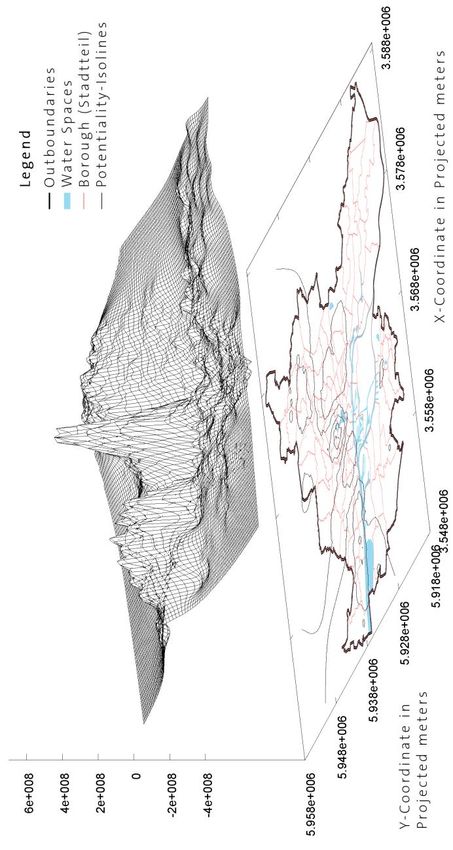
12 Gabriel M. Ahlfeldt and Arne Feddersen

                                     1. INTRODUCTION
       Top-level professional sports teams and mega-sports events represent
landmarks for their hometowns and are much appreciated by politicians aiming
at establishing identity and improving the image of their hometowns. Large
amounts of public money are spent on subsidizing representative sports venues
to improve the competitiveness of local teams or to attract mega-sports events
and major league franchises. Moreover, in recent years spectacular stadium
architecture is employed to maximize attention and to create new visiting cards
for their hometowns.1 Therefore, the impact of large sports stadiums, profes-
sional sports teams and mega-sports events has attracted much interest in scho-
larly debate.
        Empirical ex-post studies hardly find evidence for the positive impact of
sports teams and events in traditional economic terms of income, employment
and taxes, even on a city or metropolitan scale (Baade, 1988; Baade and Dye,
1990; Baade and Sanderson, 1997; Coates and Humphreys, 1999, 2003; Mathe-
son, 2008; Siegfried and Zimbalist, 2006). More recently, empirical studies
using more disaggregated data have found positive effects on location desirabil-
ity for large sports facilities within a range of up to 3 miles (4.8 km) (Ahlfeldt
and Maennig, 2008, 2009a; Coates and Humphreys, 2006; Tu, 2005). While
large facilities have been the main focus of public debates, attracting the atten-
tion of various interest groups, local authorities and neighborhood activists,
urban sports geography obviously consists of more than only representative
professional sports venues. However, with the exception of Bale (2003), mass
sports infrastructure has still found little regard in the empirical scholarly dis-
cussion. To our knowledge, no empirical evidence is available on the determi-
nants of the spatial distribution of recreational sports facilities. This is some-
what surprising in light of the widely-acknowledged positive impact of sports
on health and physical condition as well as the important role sports plays in
integrating socially disadvantaged groups. This paper aims to fill this gap by
analyzing a metropolis’ sports geography with the full diversity of all officially
registered professional, recreational, publicly and privately provided2 sports
facilities.
       Public provision of sports infrastructure is exemplary for the provision of
social infrastructure within an urban environment. Following a standard market
failure argumentation, public provision of sports facilities may be justified by
positive external effects, the merit good character and special demands of cer-
tain population groups. Moreover, referring to Alonso’s (1964) bid-rent theory,
providers of sports outlets are likely to be defeated in the competition for central
locations due to limited revenues, which, from a social planner perspective,
possibly causes underprovision in downtown areas. Our study area covers the
whole of Hamburg, Germany, presently Europe’s largest non-capital city. In its
role as the country’s second biggest city and dominating harbor metropolis, it
shares some similarities with the French city of Marseille, to which Hamburg is
1
    Ahlfeldt and Maennig (2009c) offer a survey on recent trends in stadium architecture.
2
    Privately provided sport facilities are represented by tennis courts.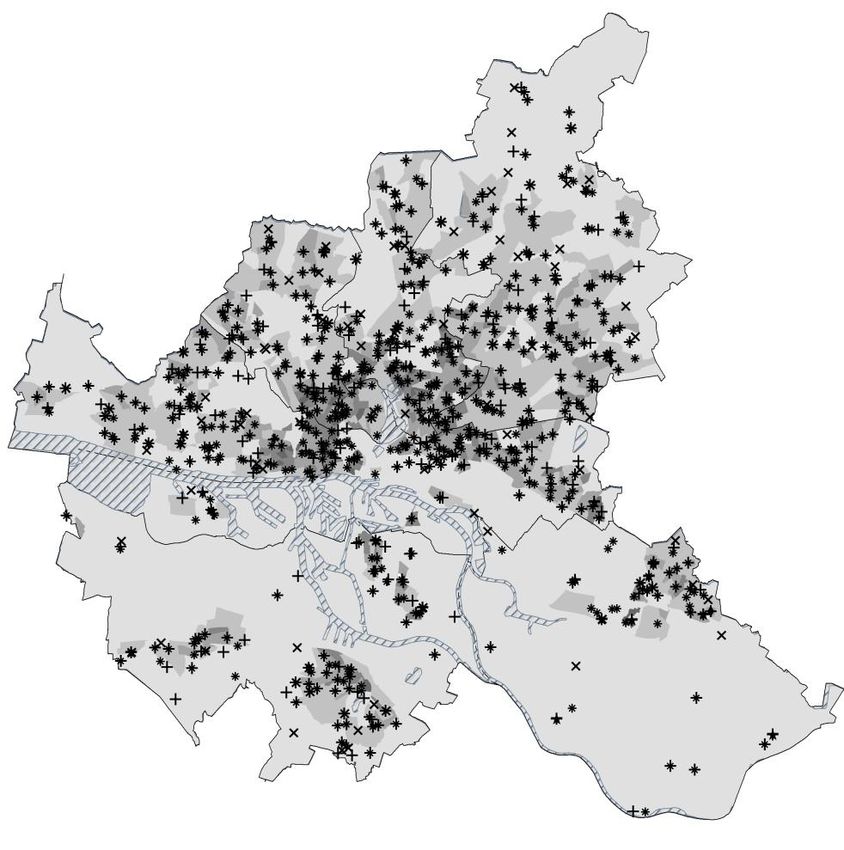
Région et Développement        13

connected by a sister-city arrangement for more than half a century. Notably,
however, Hamburg’s relative nationwide importance compared to the leading
capital city is larger than in case of the French counterpart, given that the city
features roughly 50% of the population and even 82% of the area compared to
Berlin. Moreover, Hamburg represents an ideal candidate for the evaluation of
sports infrastructural policy in Germany since local authorities keep up the
claim of Hamburg being a “sports metropolis” and should therefore be expected
to take particular care of the appropriate allocation of (public) sports infrastruc-
ture. This study assesses whether the distribution of sports facilities effectively
corresponds to the claims postulated by authorities and whether the outcome of
public provision compared to market allocation indeed justifies public provi-
sion.
       Our research strategy consists of two basic steps. First, we analyze the
spatial distribution of sports facilities in Hamburg within a theoretical frame-
work of abstract space. Sports facilities are hierarchically classified by size to
test for implications of the Sports Place Theory. Effective catchment areas are
defined based on pair-wise distances and compared to theoretical predictions
(Bale, 2003). In the second step, we relax the assumptions of plain ground and
evenly spread population to account for the obvious reality of natural and unna-
tural barriers and heterogeneity in population distribution. Employing a stan-
dard New Economic Geography concept we calculate the population potentiali-
ty representing distance-weighted population relying on effective road dis-
tances. Spatial weights are assigned according to previously assessed spatial
demand curves. Similarly, sports potentialities are created on the basis of dis-
tance-weighted sports facility size. These potentiality variables are employed to
identify the determinants of an absolute and relative location endowment with a
sports infrastructure. We introduce the concept of potentiality differentials to
assess whether market allocated sports infrastructure is concentrated in areas of
relatively higher purchasing power and whether local authorities indeed focus
on providing infrastructure in socially disadvantaged areas. Land price is also
considered in our analysis to capture opportunity cost of sports facility provi-
sion in space and to reveal whether it is a less-striking determinant in public
compared to profit-orientated provision.
       The next section presents our data. In Section 3 we test whether sports in-
frastructure follows the theoretical predictions assuming an idealized environ-
ment. The assumptions of featureless plain and homogeneity in socio-
demographic characteristics of population are relaxed in section 4 in order to
identify the determinants of locations’ absolute and relative endowment with
sports infrastructure. The final section concludes.

                                    2. DATA
       The study area covers the whole of Hamburg, which, on December 31,
2000, had 1,704,929 inhabitants and an area of approximately 755.3km2. We
collect data on 1,319 sports facilities obtained from local authorities (Sports
Office of the city of Hamburg), which we georeferenced based on addresses to
allow for spatial analysis.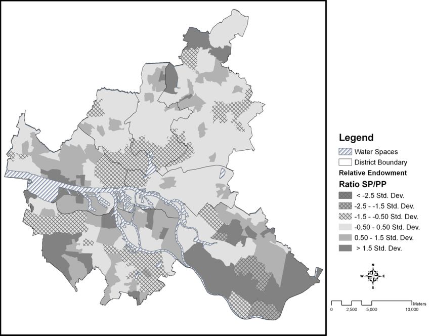
14 Gabriel M. Ahlfeldt and Arne Feddersen

    Table 1 : Descriptive statistics: Number and Size of the Sports Facilities
                                       (in m²)
                                                                      Field
                                 Halls       Fields      Tennis
                                                                     Hockey
                      N            685          495         122          17
                    Mean         428.6      8,034.5      5,231.1    15,742.4
                    Median       362.0      5,570.0      4,507.0    14,200.0
                   Std. Dev.     305.1      9,331.9      3,794.7     9,156.5
                     Min          54.0        600.0       144.0      2,100.0
                     Max       2,880.0     85,119.0    20,000.0     39,220.0

                   Figure 1 : Spatial Distribution of Sports Places

Note: Own illustration. GIS content provided by the statistical office of Hamburg and Schleswig-
Holstein.
Région et Développement       15

       We merge data on sports places with data on population, including socio-
demographic characteristics on age, income, employment and origin, disaggre-
gated to 940 officially defined statistical areas. To analyze this disaggregated
dataset, GIS tools and a projected GIS map of the official statistical area struc-
ture (statistische Gebiete) are employed enabling generation of impact variables
that are discussed in more detail in section 4. Land valuation is captured by
standard land values per square meter (Bodenrichtwerte) representing aggre-
gated market values based on property transactions within the reporting period.
We consider the most recent available data which dates to the end of 1999
(Freie Hansestadt Hamburg, 1999). Data on population and socio-demographic
characteristics refer to the end of 2000, with the exception of income, which
was only available for 1995.
                           3. ON PLAIN GROUND
3.1. Sports Place Theory
        Bale’s (2003) Sports Place Theory builds on Central Place Theory (Chris-
taller, 1933; Lösch, 1940), which is one of geography’s most prominent con-
cepts. Derived from the same assumptions of the hierarchical order of central
places, rational behavior and abstract space, the Sports Place Theory predicts
the location of sports places within an idealized world. While Bale (2003) labels
it a “normative model”, it arguably better corresponds to a classification scheme
then a theory in traditional economic understanding since it does not explain
how the predicted spatial equilibrium would emerge out of any decentralized
process (Krugman, 1996).
       The assumption of abstract space involves a plain, unbounded surface in-
habited by an evenly-spread population. On this featureless ground, sports plac-
es lie centrally within their catchment areas and provide sports outlets for their
hinterlands. Sports places can be classified according to the number of sports
provided. While small sports places have small population thresholds and cat-
chment areas, sports places of higher order need larger population thresholds for
viability. High-order places thus have larger spheres of influence, are fewer in
number and have larger distances between them. The perfect distribution of
sports facilities minimizes travel for consumers who wish to have access to the
sport they want while ensuring a minimum level of sports places’ utilization.
Such an ideal pattern is achieved by the hierarchical arrangement of central
places of different order (Christaller, 1933). Travel costs are minimized by a
lattice formed by a set of nested hexagons where spheres of influences, in con-
trast to circular spheres, do not overlap (Lösch, 1940). Figure 2 represents the
ideal organization of a sports system, the structure of which can be perfectly
described by pairwise distances between sports places of the same hierarchies
due to perfect symmetry.
3.2. Sports Hierarchies
       The demand for sports outlets diminishes with distance due to increasing
travel costs. A sports facility’s sphere of influence obviously ends where de-
16 Gabriel M. Ahlfeldt and Arne Feddersen
mand is reduced to zero. According to the Sports Place Theory, such a point,
where travel cost would become prohibitive, is a potential location for a neigh-
boring sports facility. Conversely, it is possible to infer the effective sphere of
influence from pairwise distances for sports facilities of distinct hierarchical
order.3 Considering that higher-order sports places carry out all functions pro-
vided by sports places of lower order, we derive spheres of influence derived
from pairwise distances to facilities of the same as well as higher classes.
Figure 2. Hierarchical Order of Sports Places in Abstract Space
Table 2. Mean Distance to Three Nearest Neighbors (in m)
Halls Fields Tennis All
All 731 752 2,076 566
Medium & Large 2,994 2,097 2,994
Large 5,608 5,087 4,965
Small 767 822 2,076
Medium 3,442 2,311 3,442
Incl. Large Field 1,109
Incl. Grass Field 1,129
Incl. Athletics 1,173
Incl. Hockey 4,652
Incl. Trendy 4,309
Incl. Hall 2,448
3
Assuming pairwise symmetry as in Figure 2, the distribution of central (sports) places is perfect-
ly described by distance to one of six neighbors of the same or higher class. In order to account
for the uneven distribution of facilities visible in Figure 1, an averaged distance to six neighboring
places would be suggested by the idea of a hexagonal lattice. However, we chose to restrict the
number of considered neighbors to three to avoid bias in remote areas.Région et Développement 17
Bale (2003, p. 86) suggests a sphere of influence of 800m for sports plac-
es of the lowest order and approximately 2,000m for medium-size facilities,
which is perfectly in line with our findings for open fields. However, we note
that both Bale’s prediction and our observation contradict the theoretical impli-
cation of the hexagonal lattice depicted in Figure 2, which suggests distance
between large facilities to be three times that of small ones.
4. RELAXING PLAIN GROUND
The assumption of plain ground and evenly distributed population is un-
realistic for most cities and metropolitan areas. For instance, population density
is typically higher within downtown areas compared to the urban periphery
while within the very urban core land is used almost exclusively for commercial
purposes. In the case of Hamburg, there are two additional striking particulari-
ties that contradict the assumption of abstract space. First, the rivers Alster and
Elbe represent two major natural barriers. Secondly, there is a considerable
north-south heterogeneity in the distribution of population. While Hamburg’s
north accounts for the vast majority of residents, the south is largely occupied
by industrial areas. This part of the city also hosts the harbour, which on the list
of largest European harbors features one place behind leading Rotterdam and
one place ahead of Marseille. Moreover, considerable income disparities across
space violate the assumptions of abstract space. The economic wealth of a
neighborhood possibly represents a location determinant, in particular for infra-
structure provided with the intention to make a profit. Demand for social func-
tions carried out by sports infrastructure depends on a neighborhoods’ socio-
economic characteristics, which also vary across space and need to be addressed
within an appropriate empirical framework.
4.1. Generating Potentialities
In economic geography there is a long tradition dating back to Harris
(1954) in representing the market potential by the distance-weighted sum of
population. We adopt the idea of spatial aggregation of population and approx-
imate the demand for sports infrastructure by a population potentiality measure.
For instance, let Pi be statistical area’s i population, then
PPi j
Pj exp( a d ij ) (1)
is area’s i population potentiality (PPi), where Pj is the population of area j, and
a is a distance decay factor determining the spatial weight of surrounding areas.
As we relax the assumption of plain ground we define dij as the effective road
distance between areas’ i and j geographic centroids. Statistical areas defined by
the Hamburg Senate Department differ considerably in size. Thus we employ a
basic concept of empirical economic geography (Crafts, 2005; Keeble et al.,
1982) to generate an area internal distance measure based on the surface area,
which can be used to determine the self-potential.18 Gabriel M. Ahlfeldt and Arne Feddersen
1 Area i
d ii (2)
3
where dii is block’s i internal distance equaling one-third of the radius of a circle
of block’s i surface area (Areai).
The same concept is employed to capture the sports infrastructure. In
previous research, locations’ endowments have been represented by spatially
aggregated surface areas of water bodies, green spaces and retailing centers,
which allows for relaxing the assumption of perfect substitutability of location
amenities (Ahlfeldt, 2010; Ahlfeldt and Maennig, 2009b). Similarly, we aggre-
gate the surface area of sports facilities given in square meters to obtain an indi-
cator for the spatial supply of a sports infrastructure, taking into account both
the size and proximity of all sports facilities within the neighborhood. We de-
fine sports potentiality (SPi) in statistical area i as:
SPi S j j exp( a d ij ) (3)
where Sj is the aggregated size of sports facilities in square meters within statis-
tical area j and a and dij are defined as in equation (1). When aggregating sur-
face areas across distinct types of sports facilities we normalize the surface area
by dividing by median values.
The distance-decay parameter in equations (1) and (3) determines the
weight with which the surrounding population or sports facilities enter poten-
tialities. In order to account for travel costs, more distant areas are discounted
stronger than areas in close proximity. Figure 3 shows the spatial weight func-
tions for distinct parameter values. Larger parameter values imply that sur-
rounding areas are spatially discounted stronger.
The spatial weight functions may be interpreted as spatial demand curves
revealing the spheres of influence of sports facility classes defined in section
(3.2). Bale (2003) suggests a linear demand curve as represented in Figure 3,
which declines with distance to a sports facility located at 0. At the intersection
with the x-axis, where travel costs are prohibitive for people living in 0, he pre-
dicts the location of another facility. In contrast, we assume an exponential cost
function (equations (1) and (3)) since we believe that even at relatively large
distances there is some demand remaining due to individual affiliations. We
choose decay parameters such that the half-way distances of exponential cost
functions equal one-half of the average distance to three nearest neighbors de-
termined in section (3.2) for distinct classes of sports places. At this point,
where the exponential function intersects with Bale’s (2003) linear demand
curve, the implicit spatial demand has decreased by 50%. In this way, we find
that the decay parameter of 0.5 represents a feasible approximation for medium-
class facilities. Similarly, for small and large facilities, surrounding areas are
spatially discounted employing parameter values of 1.5 and 0.25 respectively.Région et Développement 19
Figure 3. Spatial Weight Functions
The population potentiality representing the potential group of users
should be expected to be a striking determinant for spatial distribution at an
intra-urban level since the proximity to population is a major criterion in the
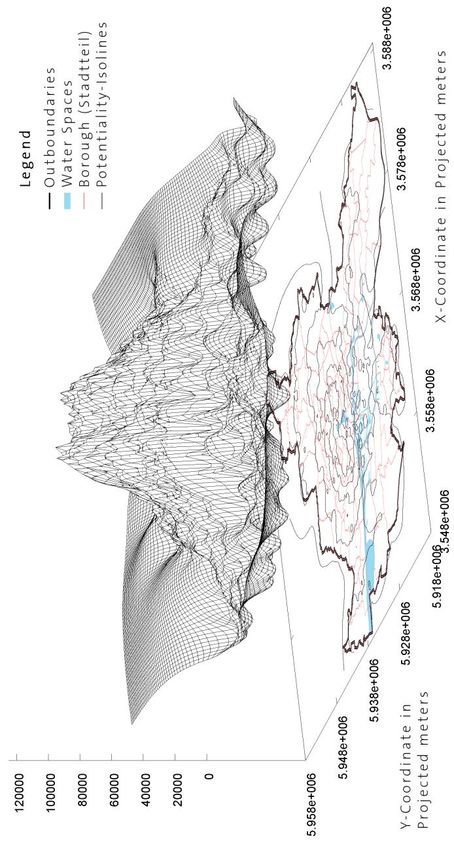
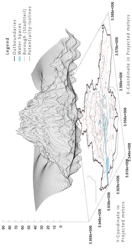
planning of publicly funded sports facilities (Ashworth, 1984). In Figure 4 and
5 we plot population and sports potentiality generated on the basis of all offi-
cially registered sports facilities in three-dimensional spaces.
Potentialities show a striking similarity, both peaking in downtown areas
and steeply descending southwards towards the river Elbe which represents a
strong natural barrier separating the densely populated areas to the north from
the industrialized south. Although sports potentiality looks slightly more ex-
panded towards the rich westward areas along the riverbank, and despite a small
heap in the south east without a counterpart in the population potentiality, these
figures clearly suggest that sports infrastructure follows the distribution of pop-
ulation.
However, particularly for the market allocated sports infrastructure, pur-
chasing power within sports facilities’ spheres of influences may be an addi-
tional location factor of relevance. We define the purchasing power of statistical
area i as the product of population and average income. In order to account for
residents being mobile across statistical areas, we capture relative economic
wealth by the potentiality difference between the current purchasing power at a
given location and a counterfactual potentiality using the average income at city
level. The purchasing power potentiality difference (PDi) at location i represents
the neighborhoods’ spatially aggregated purchasing power exceeding what
would be predicted if income was evenly distributed across space.20 Gabriel M. Ahlfeldt and Arne Feddersen
Figure 4. Population Potentiality
Notes: Figure represents population potentiality as defined in equation (1) employing a decay
parameter value of 0.5.Région et Développement 21
Figure 5. Sports Potentiality (All Facilities)
Notes: Figure represents sports potentiality as defined in equation (3) employing a decay
parameter value of 0.5.22 Gabriel M. Ahlfeldt and Arne Feddersen
Figure 6. Purchasing Power Potentiality Difference
Notes: Figure represents purchasing power potentiality difference as defined in equation (4)
employing a decay parameter value of 0.5.Région et Développement 23
PDi y P exp(a d
j j ij ) y P exp(a d
j j ij ) y j
y Pj exp( ad ij ) (4)
where yj is the average per capita income at area j and y average income at city
level.
According to the current “Leitfaden” (code of practice) of the Senate De-
partment, there is special need for supply with social infrastructure in socially
disadvantaged areas. Special need is also located in areas with a high concentra-
tion of foreigners due to the importance of sports for the process of integration.
Similarly, we apply the concept of potentiality difference to the rate of unem-
ployment, which represents a proxy for an area’s social evils. The respective
potentiality difference for unemployment, hence, indicates whether a neighbor-
hood may be regarded as socially disadvantaged compared to the Hamburg
average. Neighborhoods characterized by an above or below proportion of non-
German population are represented in the same way.
FDi F exp(a d
j ij ) f P exp(a d
j j ij ) f j
f Pj exp( ad ij ) (5)
where FDi is the potentiality difference for foreign population at area i, Fj is the
total number of foreigners within area j, fj is the proportion of foreign popula-
tion within area j and f is the same referring to the Hamburg average.
Figure (6) visualizes the purchasing power potentiality difference for
Hamburg. Income agglomerations are clearly identifiable along the Elbe river-
bank in the western part of the city and at downtown areas in proximity to the
inner-city Alster reservoir. Apparently higher-income households are willing to
bid out lower-income households at these locations, which highlights the value
of these natural amenities. Figure (6) also shows a flatter, although massive
heap in the north-east, indicating a large agglomeration of middle-high-income
households.
4.2. Empirical Strategy
Two empirical models are estimated in order to identify the determinants
of the spatial distribution of sports facilities and to assess whether systematic
disparities in the relative provision with sports infrastructure are spatially corre-
lated with neighborhood characteristics.
In model 1 we attempt to identify the major determinants of the distribu-
tion of sports facilities. Our model specification explains the sports potentiality
as defined in equation (3) by population potentiality, potentiality differences for
foreign population and purchasing power and land valuation. The price of land
represents planning authorities’ opportunity costs of providing public sports
facilities. Arguing that sports infrastructure is provided publicly to guarantee
demand-orientated allocation, property prices should not systematically influ-
ence the distribution of public sports facilities. In contrast, for non-public opera-
tors of sports facilities competing for locations on real estate markets, land price24 Gabriel M. Ahlfeldt and Arne Feddersen
is expected to be of particular relevance since the provision and operation of
sports facilities is land intensive and revenues generated by non-professional
sports are limited. Since there is typically a high spatial correlation between
land value at a given location and neighboring locations, we do not average land
value in order to obtain representative values for the neighborhood. Figure 7
represents the Moran’s I scatter plot for our land price data. There is a clearly
positive relationship between current land values and spatially weighted aver-
ages revealing the typical spillover effects in real estate markets.4
Figure 7. Morans’s I Plot
Model 1 specification thus takes following form :
SPi 1PPi 2 PDi 3 FDi 4 LVi (6)
where SPi, PPi, PDi and FDi are defined as in equations (1) - (5), LVi is mean
standard land value for area i, α and β1 to β4 represent coefficients to be esti-
mated and is an error term.5
While model 1 identifies determinants for the effective distribution of
sports facilities, model 2 focuses on areas’ relative endowments with sports
infrastructure. We create an index of sports infrastructure (ISI) on the basis of
4
Spatially weighted lags are calculated using inverse distance weights and considering three
nearest neighbors. This specification was proposed by Can and Megbolugbe (1997) and proved to
be efficient (Ahlfeldt and Maennig, 2008).
5
Due to problems of multicollinearity, the potentiality difference for unemployment is not in-
cluded into our baseline model specification.Région et Développement 25
the ratio of sports potentiality to population potentiality, which we regress on a
set of attributes capturing areas’ socio-demographic and location characteristics.
yi
ISI i 1 2ui 3uyouthi 4 f i crimei POPi a LVi (7)
y
ISIi is the ratio of sports to population potentiality for area i and yj, y , fi
and LVi are defined as in equation (1) - (5). ui is the rate of unemployment with-
in area i, uyouthi is the same for 15 to 25-year-olds, crimei is the number of
crimes committed per capita within area i and POPi is a vector of residents’
proportions of age groups.
Besides serving as a robustness check for model 1 results, this specifica-
tion allows for considering the age structure of the residential population and
additional attributes due to less problems of multicollinearity. Furthermore,
results allow for defining priorities in the planning agenda by providing recom-
mendations on how to achieve policy objectives like e.g. the integration of fo-
reigners by means of a sports infrastructural policy.
4.3. Empirical Results
4.3.1. Absolute Endowment with Sports Infrastructure
The empirical results corresponding to model 1 are represented in Table 3
to Table 5. First, we estimate equation (6) based upon the entire sample of all
1,319 sports facilities. Second, we divide the sample into several subsamples to
get a differentiated glance on different types and classes of sports facilities.
Therefore, sports facilities are differentiated by their size into small, medium
and big facilities (Table 4). To create another view, we separate sports facilities
according to their use. Thus, they are classified as sports fields (e.g. soccer,
field hockey, athletic sports), halls (e.g. team handball, basketball, volleyball,
gymnastics) and tennis courts. As the concept of potentialities derived from
equations (1) to (5) is relatively abstract, we desist from interpreting the magni-
tude of estimated coefficients. We are mainly interested in the signs and signi-
ficance levels of the coefficients since these allow for a qualitative interpreta-
tion.
Table 3. Empirical Results I (All Facilities, Model 1)
Coef. t-stat
C 5.1890 *** 17.874
PP 6.97e-4 *** 133.994
FD -7.11e-4 *** -8.873
PD -2.46e-9 *** -2.878
LV 1.17e-4 *** 1.952
R² 0.962
adj. R² 0.962
F-stat 5,498***
Notes: *** p26 Gabriel M. Ahlfeldt and Arne Feddersen
Table 3 shows a good overall fit of the model. The R² and the adjusted R²
exceed a value of 0.96 and the F-statistic is significant at the 1%-level. All coef-
ficients are significant at the 1%-level except the coefficient of the land value
(LV).
First, it is notable that the coefficient of the population potentiality is pos-
itive and highly significant, meaning that sports facilities are not evenly allo-
cated across space. After relaxing the idea of a plain ground it is fair to state that
the supply of sports facilities follows the demand deduced from the population
potential. The significantly negative sign of the foreigner potentiality difference
indicates that neighborhoods with a relatively higher proportion of non-German
population are characterized by a lower supply of sports facilities. The same
conclusion holds for the purchasing power potentiality difference. Areas with a
higher relative purchasing power have lesser sports infrastructure potentiality,
maybe indicating different preferences for a local mix of public goods and
eventually the existence of lobbying. The significantly positive sign of the coef-
ficient on LV implies that sports facilities are relatively concentrated in areas
with higher land values. This might be interpreted as a sign of local govern-
ments ignoring the opportunity cost of sports facilities supply and hence a con-
siderable divergence from the expected market solution.
A look at the subsamples confirms the findings with respect to the popu-
lation potential. The according coefficients are all positive and highly signifi-
cant. Also, an interesting pattern can be found for the purchasing power poten-
tiality difference. Distinguishing between the size of facilities and forms of
sports, a positive relation with purchasing power is only found for tennis, which
is generally known as an upper-class sport. Accordingly, tennis courts are lo-
cated in particularly wealthy areas.
Table 4. Empirical Results II (Subsamples, Model 1)
Large Facilities Medium Facilities Small Facilities
Coef. t-stat Coef. t-stat Coef. t-stat
C 0.8050 *** 3.606 2.2960 *** 12.990 0.8370 *** 9.117
PP 2.59e-4 *** 64.927 1.09e-4 *** 34.337 4.52e-5 *** 27.480
FD -9.43e-4 *** -15.303 1.03e-4 ** 2.105 5.90e-5 ** 2.326
PD -1.22e-9 * -1.853 -2.74e-9 *** -5.279 -7.71e-10 *** -2.855
LV 2.53e-4 *** 5.506 -1.67e-5 * -0.458 -9.82e-5 *** -5.195
R² 0.842 0.672 0.557
adj. R² 0.841 0.671 0.554
F-stat 1,160.376*** 445.633*** 272.959***
Notes: *** pRégion et Développement 27
cost of provision is highest in absolute terms for these kinds of sports facilities,
which provides a feasible explanation for large sports fields being located in
areas with lower land value.
Table 5 : Empirical Results III (Subsamples, Model 1)
Fields Halls Tennis
Coef. t-stat Coef. t-stat Coef. t-stat
C 21,562.260 *** 18.220 452.696 *** 5.953 3,875.667 *** 14.042
PP 1.699 *** 80.192 0.157 *** 115.616 0.243 *** 49.144
FD -6.009 *** -18.390 0.169 *** 8.065 -1.055 *** -13.841
PD -2.57e-5 *** -7.380 -1.55e-7 -0.691 8.70e-6 *** 10.722
LV -0.474 * -1.948 0.074 *** 4.730 0.027 0.482
R² 0.890 0.956 0.745
adj. R² 0.889 0.956 0.744
F-stat 1758.584 4760.051 635.949
Notes: *** p28 Gabriel M. Ahlfeldt and Arne Feddersen
age, while the degree of shading indicates the level of variation from a standard
deviation of zero in both directions. When compared to Figure 5, the advantages
of this presentation become evident. A naive view of Figure 5 suggests that the
centre of the city is well-equipped with a sports infrastructure. In contrast, Fig-
ure 8 reveals that the high-populated areas in the city center – in spite of high
provision in absolute terms – are poorly endowed with a sports infrastructure
taking into account the large potential demand. A similar pattern is found for
some of the (highly populated) subcenters like “Harburg” in the south and
“Bergedorf” in the south-east. In contrast, the wealthy area of “Blankenese”, on
the western riverbank of the Elbe, as well as the also wealthy but lower-
populated areas in the north of Hamburg can be regarded as disproportionately
highly endowed areas. Moreover, some low-populated areas display an above
average endowment, which might be attributable to the federal structure of the
city of Hamburg, where delegates of the parliament of the city have to be
(re-)elected by the voters of the district in which they are nominated.6 Lobbying
processes may explain a disproportionately high infrastructural endowment in
peripheral areas since, in federal structures, small administrative units typically
receive a relatively large proportion of delegates in the parliament and, hence,
bargaining power (Knight, 2008). In addition, relative overprovision in peri-
pheral areas is potentially amplified by the indivisibility of sports facilities.
Some quick recommendations might be derived from Figure 8. In spite of
a high sports potentiality in the city center the urban planner should – regarding
the high-population potentiality in these areas – enforce her effort in building
sports facilities there. However, besides the mere provision of sports infrastruc-
ture with respect to potential demand, one may also ask whether the (urban)
social planner is doing a good job with respect to other stated social policy ob-
jectives. In other words: Besides the absolute determinants of the spatial distri-
bution of sports infrastructure, what determines the relative endowment of sta-
tistical areas with sports facilities within the city of Hamburg?
In order to address this question, we estimate the effect of socio-
demographic factors and opportunity costs on the ratio of total sports to popula-
tion potentiality according to model 2 (Table 6). We repeat the estimates, consi-
dering only private tennis clubs, in order to identify possible differences be-
tween public and private sports facilities (Table 7).
The economic wealth of a statistical area, again, does not have a positive
impact on the provision of sports infrastructure as the coefficient of relative
income is not statistically significant, neither in variant (a) nor in variant (b).
This supports the results of model 1, where the purchasing power potentiality
difference is either negative significant or insignificant (see Table 3 to 5). Also
the overall unemployment as well as unemployment among adolescents exhibits
no significant effect. The different age groups – besides the group of 21 to 45-
year-olds – also have insignificant coefficients indicating no evidence for sys-
tematic under- or overprovision of a sports facilities. Areas with a higher crime
6
The city of Hamburg represents one of the 16 federal states of the Federal Republic of Germany
and is divided into 7 districts and 105 districts on the administrative level.Région et Développement 29
rate show an above average relative endowment of sports facilities. The crime
indicator probably captures effects related to social disadvantages, thereby also
explaining why unemployment indicators are not statistically significant at con-
ventional levels.
Figure 8. Ratio of Sports and Population Potentiality
Note: Own illustration. GIS content provided by the statistical office of Hamburg and Schleswig-
Holstein.
Table 6 shows significantly negative coefficients for the proportion of
foreign population, the proportion of middle-aged people (age group 21-45) as
well as the land value. An evident common feature of these three variables is
that they have higher values in the city center and lower values within peripher-
al areas. Therefore, the relatively low provision of sports infrastructure could be
erroneously attributed, e.g. to discrimination of foreign and middle-aged people
instead of extensive land use of sports facilities, which complicates provision in
densely developed and populated areas. We are possible only observing an ef-
fect of urban densification in statistical areas with high proportion of foreigners,
middle-aged people and with high land values.
In order to disentangle the effects of urban centrality from those of land
value and the proportion of the respective population groups, we include in
variant (b) of model 1 the effective road distance (in km) from a statistical30 Gabriel M. Ahlfeldt and Arne Feddersen
areas’ centroid to the central business district (indicated by the location of the
town hall).7 The implicit assumption which is in line with standard urban eco-
nomic models (Alonso, 1964; Mills, 1969; Muth, 1969) as well as the monocen-
tric reality in Hamburg is that the density of development decreases with dis-
tance to the urban core. Indeed, we find an inverse gradient of relative sports
facility provision, which renders the three discussed variables insignificant and
supports the hypothesis of an urban densification effect.
Table 6. Empirical Results IV (All Facilities, Model 2)
(a) (b)
Coef. t-stat Coef. t-stat
-3 -3
Constant 1.50e *** 4.139 1.17e *** 3.341
Relative Income 1.51e-8 0.153 5.28e-8 0.555
Rate of Unemployment (overall) -2.58e-6 -0.977 -1.24e-7 -0.048
Rate of Unemployment (youth) -1.75e-7 -0.068 -1.59e-6 -0.639
Proportion of Foreign Population -1.56e-6 *** -3.424 -1.44e-7 -0.310
Committed Crime per Capita 3.26e-5 ** 2.791 3.35e-5 *** 2.989
Proportion of Age Group (6y-10y) -9.69e-6 -1.227 -1.28e-5 -1.685
Proportion of Age Group (10y-15y) 2.55e-6 0.407 1.79e-6 0.297
Proportion of Age Group (15y-21y) 3.89e-6 0.913 4.04e-7 0.098
Proportion of Age Group (21y-45y) -1.02e-5 *** -2.706 -6.78e-6 * -1.853
Proportion of Age Group (45y-65y) -5.74e-6 -1.572 -3.27e-6 -0.931
Proportion of Age Group (65y+) -4.79e-6 -1.297 -3.10e-6 -0.871
Land value -5.52e-9 ** -2.259 -3.22e-9 -1.365
Road Distance to CBD -9.52e-6 *** 8.533
R² 0.242 0.302
adj. R² 0.231 0.291
F-stat 22.562*** 28.189***
N 862 862
Notes: *** pRégion et Développement 31
Comparison of Table 6 to Table 7 results yields similarities as well as dif-
ferences. First, the rate of unemployment among adolescents and most age
groups are, again, insignificant. Second, in contrast to the results for the sample
of all facilities, the proportion of older people (65 plus) is significantly negative
even though only at the 10%-level. Also, differing from Table 6, the number of
crimes committed per capita shows no significant impact for the subsample
“tennis courts”.
Table 7. Empirical Results V (Subsample: Tennis, Model 2)
(a) (b)
Coef. t-stat Coef. t-stat
Constant 1.1650 *** 2.739 0.8490 ** 2.037
Relative Income 3.77e-4 *** 3.251 4.13e-4 *** 3.653
Rate of Unemployment (overall) -0.0060 ** -2.010 -0.0040 -1.277
Rate of Unemployment (youth) -0.0020 -0.751 -0.0040 -1.226
Proportion of Foreign Population -0.0020 *** -3.780 -0.0010 -1.199
Committed Crime per Capita 0.0030 0.183 3.40e-3 0.255
Proportion of Age Group (6y-10y) -0.0030 -0.320 -0.0060 -0.656
Proportion of Age Group (10y-15y) -0.0100 -1.427 -0.0110 -1.567
Proportion of Age Group (15y-21y) -1.15e-5 -0.002 -0.0030 -0.684
Proportion of Age Group (21y-45y) -0.0120 *** -2.621 -0.0080 * -1.912
Proportion of Age Group (45y-65y) -0.0060 -1.442 -0.0040 -0.913
Proportion of Age Group (65+y) -0.0070 * -1.663 -0.0060 -1.320
Land value -7.07e-6 ** -2.465 -4.87e-6* -1.733
Road Distance to CBD -0.0090 *** 6.858
R² 0.245 0.284
adj. R² 0.234 0.273
F-stat 22.921 25.922
N 862 862
Note : *** p32 Gabriel M. Ahlfeldt and Arne Feddersen
high land values) of population groups that cluster within densely developed
downtown areas are negative significant in variant (a). Again, the hypothesis of
explicit discrimination of individual groups of the population might be rejected
in favor of an urban densification effect. The inclusion of road distance to CBD
as a control leads to the respective variables becoming almost insignificant.8
However, these findings – analogous to the previous results – suggest a signifi-
cant bias in the allocation of tennis courts, which violates the objective of so-
cially equal provision. Obviously, in favor of the planner, the same mitigating
circumstances apply as in the previous case. Moreover, the vast majority of
tennis facilities are provided privately, providing some exculpation for the plan-
ner.
5. CONCLUSION
This paper contributes to the empirical literature on the location of public
infrastructure, especially sports facilities. It also adds to the sports econom-
ics/geography literature as it serves an academic analysis of mass and recrea-
tional sports infrastructure where, so far, only studies analyzing the economic
effects of stadiums and arenas used for professional sports have been available.
In a first step, assuming plain ground and evenly distributed population, we
analyze the spheres of influence of recreational sports facilities based on the
theoretical considerations of Bale (2003). Presuming a hierarchical order of
sports places in abstract space (small, medium, and larger-sized facilities) we
provide the first empirical evidence for Bale’s (2003) theoretical predictions.
Our results suggest a sphere of influence of 752m corresponding to small sports
fields and 2,092m for medium-size fields respectively. These estimates closely
match Bale’s (2003) predictions for low (800m) and medium (2000m) order
facilities.
In the next step we relax the assumption of plain ground and evenly
spread population by applying a standard (New) Economic Geography concept,
the distance-weighted potentiality. Based on effective road distances, which
account for major natural barriers within the city boundaries of Hamburg (rivers
Elbe and Alster), and using distance decay parameters derived from the effec-
tive distribution of sports facilities, we identified the determinants of sports
facility allocation. The major findings are that: (1) the urban planner follows
population potentiality while locating the sports infrastructure; (2) areas with a
disproportionately high foreigner potentiality have lower access to recreational
sports facilities, and (3) neighborhoods’ purchasing power exhibits negligible or
negative impact on the overall endowment with a sports infrastructure, i.e. pub-
licly provided sports facilities qualify as social infrastructure.
Third, we analyzed the relative endowment of a sports infrastructure
within the framework of 940 official statistical areas. Using an index of sports
infrastructure (ISI) –the ratio of the sports potentiality and the population poten-
8
In the case of the variable Proportion of Age Group (21-45y) the coefficient is significant at the
1%-level in variant (a) and becomes significant only at the 10%-level after inclusion of the dis-
tance to the CBD in variant (b).Région et Développement 33
tiality – the previous findings from the analysis of absolute supply with sports
infrastructure were generally confirmed. In addition, the econometric analysis
of the ISI revealed some socio-demographic determinants of the relative en-
dowment of statistical areas. One of the main findings of model 2 estimations is
that – in line with the results of model 1 – purchasing power is not significant
for the sample of all sports facilities while it is significant and positive for the
tennis sample. Given that tennis facilities are largely privately provided, we
conclude that there is a significant difference in the spatial allocation between
privately and publicly provided (sports) infrastructure. It can be conjectured that
market-oriented providers of sports facilities follow purchasing power and,
hence, the customers while providers of public sports facilities follow the popu-
lation and, hence, the voters.
Another major finding of this paper is the apparent discrimination of
some social groups like non-Germans in terms of access to recreational sports
facilities. However, this reproach should be weakened since the relatively ad-
verse endowment with infrastructure is at least partially attributable to an urban
densification effect, which complicates provision within downtown areas. But
nevertheless, if the stated objective of social integration of the foreign popula-
tion by means of mass sports activities is taken for serious, then boosting en-
deavors to improve the endowment with a sports infrastructure in the respective
downtown areas is strongly recommendable.
REFERENCES
Ahlfeldt, G. M., 2010, If Alonso was right: Modelling accessibility and ex-
plaining the residential land gradient, Journal of Regional Science, forth-
coming.
Ahlfeldt G. M., Maennig W., 2008, Impact of Sports Arenas on Land Values:
Evidence from Berlin, The Annals of Regional Science, 44(2), 205-227.
Ahlfeldt G. M., Maennig W., 2009a, Arenas, Arena Architecture and the Impact
on Location Desirability: The Case of “Olympic Arenas” in Berlin-
Prenzlauer Berg, Urban Studies, 46, 1343-1362.
Ahlfeldt G. M., Maennig W., 2009b, Is the Whole More Than the Sum of Its
Parts: External Effects of Built Environment, Real Estate Economics, forth-
coming.
Ahlfeldt G. M., Maennig W., 2009c, Stadium Architecture and Urban Devel-
opment from the Perspective of Urban Economics, International Journal of
Urban and Regional Research, forthcoming.
Alonso W., 1964, Location and Land Use: Toward a General Theory of Land
Rent, Harvard University Press, Cambridge, Massachusetts.
Ashworth G., 1984, Recreation and Tourism, Bell and Hyman, London.
Baade R. A., 1988, An Analysis of the Economic Rationale for Public Subsidi-
zation of Sports Stadiums, The Annals of Regional Science, 22(2), 37-47.34 Gabriel M. Ahlfeldt and Arne Feddersen Baade R. A., Dye R. F., 1990, The Impact of Stadiums and Professional Sports on Metropolitan Area Development, Growth and Change, 21(2), 1-14. Baade R. A., Sanderson A. R., 1997, The Employment Effect of Teams and Sports Facilities, The Brookings Institute, Washington, D.C. Bale J., 2003, Sports Geography, Routledge, London. Can A., Megbolugbe I., 1997, Spatial Dependence and House Price Index Con- struction, Journal of Real Estate Finance and Economics, 14(2), 203-222. Christaller W., 1933, Central Places in Southern Germany (Baskin C. W., Trans.), Fischer, Jena. Coates D., Humphreys B. R., 1999, The Growth Effects of Sport Franchises, Stadia and Arenas, Journal of Policy Analysis & Management, 18(4), 601- 624. Coates D., Humphreys B. R., 2003, The Effect of Professional Sports on Earn- ings and Employment in the Services and Retail Sectors in U.S. Cities, Re- gional Science & Urban Economics, 33(2), 175-198. Coates D., Humphreys B. R., 2006, Proximity Benefits and Voting on Stadium and Arena Subsidies, Journal of Urban Economics, 59(2), 285-299. Crafts N., 2005, Market Potential in British Regions, 1871-1931, Regional Stu- dies, 39(9), 1159-1166. Freie Hansestadt Hamburg, 1999, Bodenrichtwertkarte 1999 von Hamburg, Gutachterausschuss für Grundstückswerte, Hamburg. Harris C. D., 1954, The Market as a Factor in the Localization of Industry in the United States, Annals of the Association of American Geographers, 44(4), 315-348. Keeble D., Owens P. L., Thompson C., 1982, Regional Accessibility and Eco- nomic Potential in the European Community, Regional Studies, 16(6), 419- 431. Knight B., 2008, Legislative Representation, Bargaining Power and the Distri- bution of Federal Funds: Evidence from the US Congress, The Economic Journal, 118(532), 1785-1803. Krugman P., 1996, The Self-Organizing Economy, Blackwell, Cambridge. Lösch A., 1940, The Economics of Location, Fischer, Jena. Matheson V., 2008, Mega-Events: The Effect of the World's Biggest Sporting Events on Local, Regional, and National Economies, in Howard D., Humph- reys B., editors, The Business of Sports, Vol. 1, 81-97, Praeger Publishers, New York. Mills E. S., 1969, The Value of Urban Land, in Perloff H., editor, The Quality of Urban Environment, Resources for the Future, Inc., Baltimore, MA.
Région et Développement      35

Muth R. F., 1969, Cities and Housing: The Spatial Pattern of Urban Residential
  Land Use, University of Chicago Press, Chicago.
Siegfried J., Zimbalist A., 2006, The Economic Impact of Sports Facilities,
   Teams and Mega-Events, Australian Economic Review, 39(4), 420-427.
Tu C. C., 2005, How Does a New Sports Stadium Affect Housing Values? The
   Case of Fedex Field, Land Economics, 81(3), 379-395.

       LA LOCALISATION DES INSTALLATIONS SPORTIVES
             DANS LA MÉTROPOLE DE HAMBOURG

Résumé - Cet article étudie la localisation des infrastructures sportives dans la
ville de Hambourg, en s’appuyant sur une base de données de 1319 installa-
tions. Il montre, dans un premier temps, que les quartiers centraux sont, de
façon générale, relativement dépourvus d’infrastructures sportives, du fait des
coûts fonciers prohibitifs. Dans un deuxième temps, l’article tente d’expliquer
la localisation des installations sportives selon leur nature. Les installations
nécessitant une forte emprise foncière (par exemple les stades de football) se
trouvent en périphérie, non seulement par calcul économique, mais également
parce qu’elles correspondent à des activités sportives plutôt exercées par des
ménages à revenu faible ou moyen. A l’inverse, les installations sportives ré-
clamant peu d’espace, comme le tennis, se rapprochent du centre-ville, car elles
correspondent également aux préférences des ménages à revenu plus élevé.
You can also read