Global agricultural ammonia emissions simulated with the ORCHIDEE land surface model
←
→
Page content transcription
If your browser does not render page correctly, please read the page content below
Model description paper
Geosci. Model Dev., 16, 1053–1081, 2023
https://doi.org/10.5194/gmd-16-1053-2023
© Author(s) 2023. This work is distributed under
the Creative Commons Attribution 4.0 License.

Global agricultural ammonia emissions simulated with the
ORCHIDEE land surface model
Maureen Beaudor1 , Nicolas Vuichard1 , Juliette Lathière1 , Nikolaos Evangeliou2 , Martin Van Damme3,4 ,
Lieven Clarisse3 , and Didier Hauglustaine1
1 Laboratoire des Sciences du Climat et de l’Environnement (LSCE), CEA–CNRS–UVSQ, Gif-sur-Yvette, France
2 Department  of Atmospheric and Climate Research (ATMOS), Norwegian Institute for Air Research (NILU), Kjeller, Norway
3 Spectroscopy, Quantum Chemistry and Atmospheric Remote Sensing (SQUARES),

Université libre de Bruxelles (ULB), Brussels, Belgium
4 Royal Belgian Institute for Space Aeronomy, Brussels, Belgium

Correspondence: Maureen Beaudor (maureen.beaudor@lsce.ipsl.fr)

Received: 11 July 2022 – Discussion started: 5 September 2022
Revised: 20 January 2023 – Accepted: 24 January 2023 – Published: 9 February 2023

Abstract. Ammonia (NH3 ) is an important atmospheric con-        a 10 % change in emissions per percent change in pH. Even
stituent. It plays a role in air quality and climate through     though we found an underestimation in our emissions over
the formation of ammonium sulfate and ammonium nitrate           Europe (−26 %) and an overestimation in the USA (+56 %)
particles. It has also an impact on ecosystems through depo-     compared with previous work, other hot spot regions are con-
sition processes. About 85 % of NH3 global anthropogenic         sistent. The calculated emission seasonality is in very good
emissions are related to food and feed production and, in        agreement with satellite-based emissions. These encourag-
particular, to the use of mineral fertilizers and manure man-    ing results prove the potential of coupling ORCHIDEE land-
agement. Most global chemistry transport models (CTMs)           based emissions to CTMs, which are currently forced by
rely on bottom-up emission inventories, which are subject        bottom-up anthropogenic-centered inventories such as the
to significant uncertainties. In this study, we estimate emis-   CEDS (Community Emissions Data System).
sions from livestock by developing a new module to calcu-
late ammonia emissions from the whole agricultural sector
(from housing and storage to grazing and fertilizer applica-
tion) within the ORCHIDEE (Organising Carbon and Hy-             1   Introduction
drology In Dynamic Ecosystems) global land surface model.
We detail the approach used for quantifying livestock feed       Ammonia (NH3 ) is a crucial species in the atmosphere, play-
management, manure application, and indoor and soil emis-        ing a role in the alteration of air quality and climate through
sions and subsequently evaluate the model performance. Our       its implication in airborne particle matter formation (PM or
results reflect China, India, Africa, Latin America, the USA,    aerosols) (Anderson et al., 2003; Bauer et al., 2007). The
and Europe as the main contributors to global NH3 emis-          NH3 lifetime is short and has been reported to range from
sions, accounting for 80 % of the total budget. The global       a few hours to a few days (Pinder et al., 2008; Behera et al.,
calculated emissions reach 44 Tg N yr−1 over the 2005–2015       2013), as ammonia mostly originates from surface emissions
period, which is within the range estimated by previous work.    and its deposition velocity is high over most surfaces (Hov
Key parameters (e.g., the pH of the manure, timing of N ap-      et al., 1994; Evangeliou et al., 2020). Due to this character-
plication, and atmospheric NH3 surface concentration) that       istic, NH3 is transported over relatively short distances and
drive the soil emissions have also been tested in order to as-   readily reacts with abundant gases such as nitric and sulfuric
sess the sensitivity of our model. Manure pH is the parame-      acids to form secondary aerosols (Malm et al., 2004). The
ter to which modeled emissions are the most sensitive, with      resulting aerosols, such as ammonium nitrates or ammonium
                                                                 sulfates, have important impacts on the Earth’s radiative bud-

Published by Copernicus Publications on behalf of the European Geosciences Union.
1054                               M. Beaudor et al.: Global agricultural ammonia emissions simulated with ORCHIDEE

get due to their ability to scatter incoming radiation, act as      housing conditions, temperature, and animal waste handling
cloud condensation nuclei, and indirectly increase cloud life-      practices (Anderson et al., 2003). The soil NH3 emissions
time (Abbatt et al., 2006; Henze et al., 2012; Behera et al.,       originate from N application, either from fertilizer or manure,
2013; Evangeliou et al., 2020). The impact of NH3 on the to-        and are controlled by the soil pH, temperature, water content,
tal radiative forcing is estimated to be −0.06 W m−2 , with re-     surface wind speed, and the atmospheric NH3 concentration
spective contributions of about −0.07 and 0.01 W m−2 to the         (Kirk and Nye, 1991; Hertel et al., 2011; Behera et al., 2013).
radiative forcing of nitrate and sulfate (Myhre et al., 2013).      Other factors such as the ammonium content of the fertilizer
By analyzing different Representative Concentration Path-           and the timing of N application are also crucial for emission
way (RCP) scenarios, Hauglustaine et al. (2014) showed the          estimates (Riddick et al., 2016; Vira et al., 2020).
importance of ammonia with respect to the direct aerosol               The first type of approach to the quantification of agri-
forcing in the future due to the potentially significant increase   cultural ammonia emissions is bottom-up inventories. Most
in agricultural emissions. In the most extreme scenario, emis-      global inventories, such as the CEDS (Community Emis-
sions could increase by 50 % by 2100 compared with their            sions Data System; McDuffie et al., 2020), EDGAR (Emis-
present-day level.                                                  sions Database for Global Atmospheric Research; Crippa
   In addition to its contribution to the radiative budget, the     et al., 2018), and HTAP (Hemispheric Transport of Air Pollu-
balance between NH3 , SO2 , and NOx emissions controls the          tion; Janssens-Maenhout et al., 2015), are based on activity
formation of secondary inorganic aerosols (SIAs), which are         data associated with corresponding emission factors (EFs).
important components of fine particles (PM2.5 ) (Paulot et al.,     Chemistry transport models (CTMs) are usually forced with
2016; Fu et al., 2017; Sutton et al., 2020). Quantifying am-        these global emission inventories. As examples, the inven-
monia emissions is of high interest for air quality policies, as    tory described by Bouwman et al. (1997) is prescribed in
it appears that NH3 emission reductions would also be effi-         the study of Xu and Penner (2012), and the CEDS inven-
cient to reduce inorganic aerosol formation (Lachatre et al.,       tory (McDuffie et al., 2020) is used in Paulot et al. (2016)
2019).                                                              and Pai et al. (2021). Emission inventories do not account
   There are many issues in the development of reliable             for environmental factors, such as the temperature or soil hu-
NH3 emission inventories, as analyzed by Nair and Yu                midity, which is an important limitation for studying spatial–
(2020), such as the lack of emission measurements, the dif-         temporal variability in the atmospheric NH3 and NH+      4 con-
ficulties in validating the NH3 concentration with measure-         centrations. Most inventories rely on the fertilizer applica-
ments, and the critical assumptions behind the modeling             tion period to represent the seasonality of emissions but
approaches in terms of emission factors and activity rates.         are based on few studies and usually use the same tempo-
Even though ammonia emissions are challenging to esti-              ral profile (most of the time reflecting European agricul-
mate, several studies have aimed at quantifying global emis-        tural practices), which is extrapolated to the whole globe.
sions and their associated uncertainty. For example, Den-           More complex inventories exist, such as the updated version
tener and Crutzen (1994) estimated a global NH3 emission            of the Global Livestock Environmental Assessment Model
of 45 Tg N yr−1 (±50 %), which is a low estimate compared           (GLEAM; Uwizeye et al., 2020) or the comprehensive food
with the 54 Tg N yr−1 (±25 %) of Bouwman et al. (2005)              system developed by Conijn et al. (2018), and combine more
and the 75 Tg N yr−1 (±50 %) of Schlesinger and Hartley             detailed agricultural information (e.g., animal requirements,
(1992) (Zhu et al., 2015). Agricultural activities are among        livestock system types, manure management, and the sur-
the significant sources of ammonia in the world, accounting         face types receiving manure) with EFs but consider yearly
for about 85 % of the global anthropogenic NH3 emissions            emissions. Even though this type of approach is more accu-
(Behera et al., 2013). Agricultural emissions originate from        rate due to the detailed consideration of agricultural prac-
fertilizer application and livestock management, with the lat-      tices, it shows limitations for studying the temporal vari-
ter including livestock housing, manure storage, and manure         ability in emissions due to the static representation of the
application. Globally, recent studies have developed method-        agricultural practices when using unique EFs or only one
ologies in order to quantify emissions from this sector. For        seasonal profile for the whole globe. Recently, more com-
example, Beusen et al. (2008), Paulot et al. (2014), and Mc-        plex models based on an explicit description of processes
Duffie et al. (2020) estimated similar emissions of about 32–       that control the volatilization from soil have been developed.
35 Tg N yr−1 , which is less than the 41–47 Tg N yr−1 esti-         The FAN (Flow of Agricultural Nitrogen) model, initially
mates of Crippa et al. (2018) and Vira et al. (2020).               developed by Riddick et al. (2016) and largely improved
   Modeling NH3 sources from agriculture is especially dif-         by Vira et al. (2020), combines information on agricultural
ficult because it depends on several factors related to the         practices, emission factors for manure management emis-
environment (e.g., atmospheric conditions and soil proper-          sions, and physical processes for soil volatilization to com-
ties) and to agricultural practices, which are also crucial to      pute NH3 emissions from the different agricultural sources.
capture the temporal and spatial variability in emissions cor-      When soil processes are tightly coupled to the main me-
rectly. Emissions from manure management are driven by the          teorological drivers, the related emissions respond to envi-
amount of N in the feed, animal body characteristics, animal        ronmental changes, which is particularly interesting in the

Geosci. Model Dev., 16, 1053–1081, 2023                                             https://doi.org/10.5194/gmd-16-1053-2023

M. Beaudor et al.: Global agricultural ammonia emissions simulated with ORCHIDEE                                            1055

case of climate–surface interaction studies. Even if the FAN      (PFTs), among which two crop types (C3 and C4 ) and four
model is integrated into the Community Earth System Model         grass types (temperate, boreal, and tropical C3 grasses as
(CESM), the manure produced by livestock is not directly          well as a single C4 class) are represented. The initial version
linked to the biomass productivity, which can represent un-       used in this study includes a simple management of the crop
certainty in the N content of the manure and, therefore, in the   biomass (which assumes that 45 % of the net primary pro-
resulting emissions.                                              ductivity, NPP, is harvested) but no grassland management.
   In this study, in order to better account for the key param-      The main N processes within the soil–plant–atmosphere
eters in the estimate of the NH3 emissions, we implement a        continuum are based on the OCN model (Zaehle and Friend,
module representing the agricultural sector within the OR-        2010; Zaehle et al., 2010). The representation of nitrifica-
CHIDEE (Organising Carbon and Hydrology In Dynamic                tion and denitrification processes are based on the DNDC
Ecosystems) land surface model (LSM). Our methodology             (DeNitrification–DeComposition) model (Li et al., 1992; Li,
is based on the integration of a complete dynamical agricul-      2000; Zhang et al., 2002). It accounts for ammonia/ammo-
tural module (CAMEO, Calculation of AMmonia Emissions             nium (NH3 /NH+                      −
                                                                                    4 ), nitrate (NO3 ), nitrogen oxides (NOx ),
in ORCHIDEE) within ORCHIDEE, which details a feed                and nitrous oxide (N2 O) pools as well as the related emis-
management module linked to the biomass productivity of           sions. In addition to NH3 , NOx , N2 O, and N2 emissions, N
the model and animal characteristic information, a manure         is lost through runoff and leaching processes. The N inputs to
management representation that combines regional agricul-         soil mineral pools include atmospheric NOy and NHx depo-
tural handling practices, and a complex soil emission com-        sition, biological nitrogen fixation (BNF), and the application
ponent based on key environmental parameters such as the          of synthetic and organic fertilizers over agricultural lands.
vegetation growth, temperature, and soil humidity.                The total ammonia nitrogen (TAN) pool is also updated ac-
   Section 2 describes the agricultural model within OR-          cording to plant uptake, as described in Zaehle and Friend
CHIDEE and the model setup of the 11 year control simula-         (2010). The version of ORCHIDEE used for this study is
tion (2005–2015) as well as with the sensitivity analysis sim-    ORCHIDEEv3, revision 6863. It was part of the ensemble of
ulation set. Global and regional results comparing previous       terrestrial ecosystem models used for the 2019 Global Car-
works (CEDS and the FAN model from Vira et al., 2020) and         bon Budget (Friedlingstein et al., 2019) and was recently
seasonal analysis using airborne measurements (Infrared At-       evaluated by Seiler et al. (2022). Overall, ORCHIDEEv3
mospheric Sounding Interferometer-derived emissions) are          shows good agreement with observation-based data for car-
presented and discussed in Sect. 3. The conclusions are pro-      bon fluxes and vegetation state. Former revisions of OR-
vided in Sect. 4.                                                 CHIDEEv3 have also been used to quantify the global gross
                                                                  primary production (GPP) flux (Vuichard et al., 2019) and
                                                                  soil N2 O emissions (Tian et al., 2018). In the initial version,
2     Methods                                                     the organic fertilizer (i.e., manure) amount was prescribed
                                                                  annually (Zhang et al., 2017a), and the corresponding quan-
This section describes the process-based model for the N
                                                                  tity of N was applied at a constant rate daily over the whole
flow from agriculture within the ORCHIDEE LSM. The new
                                                                  year. In addition, the emissions from the whole manure man-
module implemented here aims at calculating two types of
                                                                  agement were missing, and only soil emissions were taken
emissions from agriculture: the manure management chain
                                                                  into account. A description of the ORCHIDEE model, in-
emissions (livestock housing and yard emissions as well
                                                                  cluding the nitrogen cycle and its interaction with the car-
as manure storage emissions) and soil emissions (account-
                                                                  bon cycle, is detailed in Vuichard et al. (2019). At the global
ing for fertilizer and manure application). The ORCHIDEE
                                                                  scale, the model evaluation shows good agreement between
model framework is described in Sect. 2.1.1 followed by the
                                                                  the gross primary production simulated with the carbon–
different interactive components (shown in Fig. 1): the feed-
                                                                  nitrogen interaction version and the observational validation
ing of livestock, the whole manure management chain, fertil-
                                                                  set.
izer surface application, and the soil–plant–atmosphere con-
                                                                     In this paper, we integrate the following new developments
tinuum processes leading to soil emissions. Section 2.2 de-
                                                                  within a new module called CAMEO for the Calculation of
scribes the setup of the simulations and the model evaluation
                                                                  AMmonia Emissions in ORCHIDEE:
protocol.
                                                                    – a new grassland and cropland management module ded-
2.1     The ORCHIDEE LSM                                              icated to livestock feeding (Sect. 2.1);
2.1.1    General description                                        – a module computing manure production and the associ-
                                                                      ated emissions from indoor farming livestock activities
ORCHIDEE is a global-scale terrestrial ecosystem model                (housing, yard, manure storage) (Sect. 2.1);
coupling energy, water, and both the carbon and nitro-
gen cycles (Ciais et al., 2005; Krinner et al., 2005; Piao          – a new parametrization for agricultural N application
et al., 2007). Vegetation comprises 15 plant functional types         onto croplands and grasslands (Sect. 2.1);

https://doi.org/10.5194/gmd-16-1053-2023                                            Geosci. Model Dev., 16, 1053–1081, 2023
1056                                 M. Beaudor et al.: Global agricultural ammonia emissions simulated with ORCHIDEE

  – an improved soil emission scheme based on a more re-           (Table 2), and the 0.32 factor corresponds to the C content
    alistic representation of the soil–plant–atmosphere con-       of straw, assuming a C : N ratio of 80 (USDA, 2022) for the
    tinuum (Sect. 2.1).                                            straw material and an N content of 4 g N kg−1 (EMEP/EEA,
                                                                   2019). This value is consistent with recent experimental
2.1.2   The agricultural N-flow module within                      studies by Su et al. (2020), who found 0.35 kg kg−1 of total
        ORCHIDEE: CAMEO                                            carbon in wheat straw.
                                                                      BMbedding (a) and BMing,crop(a) constitute the total demand
Livestock feed management                                          for crops. We assume that the demand for crop biomass in
                                                                   each grid cell is satisfied by the amount of crop biomass
Both the livestock feeding (BMing , kg C m−2 yr−1 ) and bed-       harvested globally (global market). In contrast, the grass
ding (BMbedding , kg C m−2 yr−1 ) needs are calculated within      biomass needs are satisfied locally. Indeed, the grass biomass
each grid cell from livestock density distribution maps, for       needs define the grassland management intensity through a
different livestock categories. The livestock types considered     grazing indicator (GI, unitless) that corresponds to the frac-
in our study are non-dairy cattle, dairy cattle, pigs, small ru-   tion of grass NPP for the year y that is harvested. Hence, the
minants, and chickens, which are the main contributors to          GI is defined as follows:
global livestock NH3 emissions. Da , the distribution of each
livestock category a, is taken from the Gridded Livestock of                         BMing grass
                                                                   GI(y) = min                      ; maxabove ,               (4)
the World (GLW 2; Robinson et al., 2014) for the year 2006.                       NPPgrass above(y)
   BMing for livestock category a is calculated as follows:
                                                                   where NPPgrass above(y) corresponds to the above NPP of
BMing (a) = Da × SI × Wa ,                                  (1)    grasslands at the grid cell level (kg C m−2 per grid cell per
where Wa is the animal weight (kg), and SI is the specific         year) and maxabove , which is a parameter equal to 0.7 and
intake (the intake per animal weight unit, kg C kg−1 yr−1 ).       defined as the maximum of the above biomass available for
   A daily dry matter intake equal to 2.5 % of the livestock       grazing/cutting.
weight (Paustian et al., 2006) is considered for every live-          NPPgrass above(y) is a function of the grassland NPP
stock category, and a factor of 0.45 is used to convert the        (kg C m−2 per grassland per year) but also of the grassland
dry matter into carbon matter (Paustian et al., 2006), leading     area defined in each grid cell. Due to an inconsistency be-
to an SI value of 0.01 kg C kg−1 yr−1 . Regarding livestock        tween the land use map and livestock density map, the tar-
weights, we use regional values adapted from the Supple-           geted BMing grass value may not be reached by the use of the
ment of FAO (2018), as listed in Table 1.                          GI. To ensure that BMing grass demand is always satisfied, we
   The livestock feeding and bedding needs are provided by a       adjust the diet composition of ruminants in some grid cells
fraction of the crop and grass NPP which is harvested (called      by increasing dcrop (a) as much as needed (and by reducing
BMharv/graz ). In order to quantify the amount of grassland        dgrass (a) by the same factor). The adjusted value of dgrass (a)
and cropland biomass needed to feed each livestock category        is named dgrass, adjusted (a) and is depicted in the Supple-
(BMing,grass (a) and BMing,crop (a) , respectively), we use the    ment (Fig. S1). The GI is then applied to NPPgrass above(y)
fractions of grass and crop that constitute the diet compo-        on a daily basis in order to obtain the total effective grazed
sition of each animal (dgrass (a) and dcrop (a) , respectively).   biomass. For each animal, dgrass, adjusted (a) is used to deduce
The ruminant animals (i.e., cattle and small ruminants) have       the effective crop biomass from the effective grazed biomass.
a diet composed of a portion of grass and crop, whereas the        Finally, each grid cell’s effective crop biomass is constrained
non-ruminant animals (i.e., pigs and chickens) have a crop-        by the global crop harvested NPP. To do so, we compute
only diet. The bedding needs are taken from crop residues          the ratio between the global effective crop biomass and the
only.                                                              global crop harvested NPP (HI) at a yearly time step. When
                                                                   HI > 1, we impose the same constraint locally by dividing
BMing,grass(a) = BMing(a) × dgrass   (a)                           the effective crop biomass by HI.
BMing,crop(a) = BMing(a) × dcrop   (a)                      (2)       As our methodology is based on an N-flow scheme, the
                                                                   C : N ratio imposed by the model for the crop and grass prod-
The diet composition dcrop/grass (a) is calculated from re-        ucts is used to convert the carbon into the N biomass ingested
gional feeding information detailed in the Global Livestock        (in kg N m−2 yr−1 ). The grassland C : N ratio is unique for
Environmental Assessment Model (FAO, 2018) and is de-              each grid cell and varies spatially from 23 to 62, whereas the
scribed in the Supplement. The bedding is estimated as fol-        cropland C : N ratio is fixed for the whole globe and is esti-
lows EMEP/EEA (2019):                                              mated to be ∼ 38. BMing tot(y,a) represents the total (includ-
BMbedding (a) = Da × 0.32 × Strawa .                        (3)    ing crop and grass products) N biomass ingested, which is
                                                                   used to compute the resulting manure emissions (described
Here, Strawa corresponds to the amount of straw                    in the next section). Concerning the crop used as straw, a
(kg head−1 yr−1 ) used as bedding for each livestock type          fixed C : N ratio of 80 is chosen (EMEP/EEA, 2019).

Geosci. Model Dev., 16, 1053–1081, 2023                                            https://doi.org/10.5194/gmd-16-1053-2023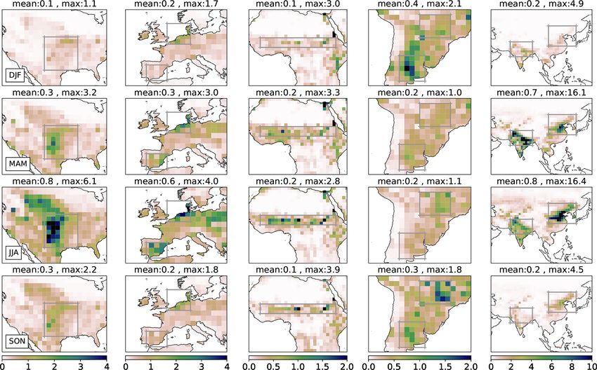
M. Beaudor et al.: Global agricultural ammonia emissions simulated with ORCHIDEE                                                        1057

Figure 1. Scheme of the agroecosystem representation developed within ORCHIDEE. It is composed of four main components describing
feed management, manure management, surface N application, and the soil–plant–atmosphere continuum processes leading to the soil
emissions. The livestock distributions and synthetic fertilizers are the main forcing files in the system and are represented in the dashed
frames. The time steps (1 year, 1 d, and 30 min) of the processes are indicated using the arrows.

Table 1. Regional weights of the animal (kg) used in the intake needs calculation. Data have been adapted from FAO (2018). The regions
listed in the table are as follows: NA (North America), RUS (Russian Federation), WE (western Europe), EE (eastern Europe), NENA (Near
East and North Africa), ESEA (East and Southeast Asia), OCE (Oceania), SA (South Asia), LAC (Latin America and the Caribbean), and
SSA (sub-Saharan Africa).

                                         NA     RUS     WE     EE     NENA      ESEA     OCE      SA     LAC     SSA
                     Dairy cattle        750     500    594    514       370      398      461    336     556     287
                     Non-dairy cattle    744     611    611    610       407      482      440    409     556     296
                     Pigs                157     142    163    148       117      103      113     91     143      72
                     Chickens             1.5     1.7   1.9    1.8       1.6      1.7      1.7    1.4     1.6     1.7
                     Small ruminants       85      77    75     76        50       40       76     39      60      34

Indoor N flows and ammonia emissions                                    Secondly, we compute the manure excreted during the dif-
                                                                        ferent livestock activities as a proportion of the year spent
We adapt the scheme developed by Dämmgen and Hutch-                     in housing, in the yard, and grazing, based on EMEP/EEA
ings (2008) which defines indoor ammonia emissions for                  (2019). The fraction of time spent in the yard (xyard , Table 2)
each animal category. These pathways have also been used                is prescribed. The remaining time fraction is split into graz-
in the Tier 2 methodology of the manure management part                 ing (xgraz , Table 2) and housing periods.
of the EMEP/EEA Air Pollutant Emission Inventory Guide-
book EMEP/EEA (2019). It is based on an N-flow model                    mN (yard,a) = xyard,a × mexcreted(a)
with mass transfers and emissions proportional to the TAN.              mN (graz,a) = xgraz,a × (1 − xyard,a ) × mexcreted(a)
   The main output of this module is the N emissions that
                                                                        mN (house,a) = (1 − xgraz,a ) × (1 − xyard,a ) × mexcreted(a)    (6)
occur during housing, yarding, and storage of animals, along
with the resulting manure produced. The seasonal variability            Default values of the TAN fraction contained in the exc-
in indoor N emissions is neglected, and the emissions and the           retal N (xTAN,a ) from the manure management part of the
manure flow are calculated yearly.                                      EMEP/EEA Air Pollutant Emission Inventory Guidebook
   Firstly, we compute the N biomass excreted by each an-               2019 (EMEP/EEA, 2019) (see Table 2) are used to calculate
imal category (mexcreted ) based on the excretion rates esti-           the amount of TAN produced during each activity, i (hous-
mated by Paustian et al. (2006) for the Intergovernmental               ing, yarding, and grazing):
Panel on Climate Change (IPCC) Tier 2 recommendations
(see Table 2).                                                          mTAN (i,a) = xTAN,a × mN(i,a) .                                  (7)

mexcreted(a) = BMing tot(y,a) × (1 − Nretained(a) )            (5)

https://doi.org/10.5194/gmd-16-1053-2023                                                   Geosci. Model Dev., 16, 1053–1081, 2023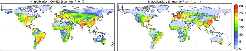
1058                                  M. Beaudor et al.: Global agricultural ammonia emissions simulated with ORCHIDEE

Table 2. Default values for the fractions of the year spent grazing and in the yard, the proportion of TAN in the N mass retained, and the straw
used as bedding. The information has been taken and adapted from EMEP/EEA (2019). The straw used as bedding for pigs is the average
between different livestock types. The N retained is taken from Paustian et al. (2006).

                                                     xgraz     xyard      N retained       xTAN                  Straw
                                                       (–)       (–)         (–)            (%)       (kg head−1 yr−1 )
                                Dairy cattle           0.5      0.25        0.20             60                      1500
                                Non-dairy cattle       0.5      0.10        0.07             60                       500
                                Pigs                     0         0        0.30             70                       400
                                Chickens                 0         0        0.30             70                      0.00
                                Small ruminants       0.92      0.02        0.10             50                        20

   mTAN (graz,a) and mN (graz,a) are used in Sect. 2.1 for N ap-              at a rate fimm proportional to mbed,N,a . An fimm value
plication on cultivated areas.                                                of 0.0067 kg kg−1 is used (Kirchmann and Witter, 1989;
   The ammonia emissions from housing ENH3 (house,a)                          Webb and Misselbrook, 2004; EMEP/EEA, 2019). This
(in kg N m−2 yr−1 ) combine the volatilization from liq-                      immobilization greatly reduces the resulting NH3 emissions.
uid and solid TAN masses, with specific emission fac-
tors: EFNH3 (house,liq,a) (kilograms of NH3 -N per kilogram of                mN (stor,liq,a) = (mN (house,liq,a) − ENH3 (house,liq,a) )
TAN) and EFNH3 (house,sol,a) (kilograms of NH3 -N per kilo-                   + (mN (yard,a) − ENH3 (yard,a) );
gram of TAN). EFNH3 (house,liq,a) and EFNH3 (house,sol,a) val-                mTAN (stor,liq,a) = (mTAN (house,liq,a) − ENH3 (house,liq,a) )
ues are taken from Sommer et al. (2019) for each animal a
                                                                              × (1 − fmin )+
except for the small ruminants category, which is assigned a
value from EMEP/EEA (2019) (see Table 3). ENH3 (house,a) is                   mTAN (stor,liq,a) × fmin + (mTAN (yard,a) − ENH3 (yard,a) );
written as follows:                                                           mN (stor,sol,a) = mN (house,sol,a) − ENH3 (house,sol,a)
ENH3 (house,a) = (xliq,a × EFNH3                                              + mbed,N,a ;
                                    (house,liq,a) + (1 − xliq,a )
               × EFNH3 (house,sol,a) ) × mTAN (house,a) ,           (8)       mTAN (stor,sol,a) = mTAN (house,sol,a) − ENH3 (house,sol,a)
                                                                              − mbed,a × fimm .                                                     (10)
where xliq,a (unitless) is the proportion of manure handled as
liquid for livestock type a, adapted from the Global Live-                    Here, mbed,N is the N mass of bedding (kg N m−2 yr−1 ), and
stock Environmental Assessment Model (FAO, 2018) (see                         mbed is the dry matter mass of bedding.
Supplement).                                                                     Manure from storage is supposed to be entirely used as
   Emissions from yarding (ENH3 (yard,a) ) are calculated from                fertilizer. The quantities mTAN (applic) and mN (applic) are the
the mass excreted in the yard, and there is no distinction be-                respective TAN and N manures that will be applied to the sur-
tween liquid and solid handling.                                              face, as described in Sect. 2.1. They are obtained by remov-
                                                                              ing the total N emissions from the stored manure (Eq. 11).
ENH3 (yard,a) = EFNH3    (yard,a) × mTAN (yard,a)                   (9)

                                                                                           mTAN (applic,liq,a) = mTAN (stor,liq,a) − Estor(liq,a)
                                                                              liquid       mN (applic,liq,a) = mN (stor,liq,a) − Estor(liq,a)
   We compute the amounts of N and TAN that are stored
as liquid and solid before application (mN (stor,type,a)                                   mTAN (applic,sol,a) = mTAN(stor,sol,a) − Estor(sol,a)
                                                                               solid       mN (applic,sol,a) = mN(stor,sol,a) − Estor(sol,a)        (11)
and mTAN (stor,type,a) for type=liq,sol, respectively;
kgNm−2 yr−1 ; Eq. 10). For storage, we assume that all                           In addition to emissions of NH3 , other N species (N2 O,
of the manure from housing and yarding is stored, except                      NO, and N2 ) emissions can occur from storage and, thus,
the N lost by ammonia emissions in the house and yard                         are required to calculate the final manure mass from storage.
(ENH3 (house,a) and ENH3 (yard,a) , respectively). Manure from                These emissions are obtained using the EFs listed in Table 3
yarding is considered liquid and goes in the liquid manure                    as follows:
storage. Concerning the liquid storage (i.e., slurries), a
fraction fmin of the organic N (N-TAN) is converted into                      Estor,liq,a = mTAN (stor,liq,a) ×
TAN through mineralization. A value of 0.1 is used for fmin                                 (EFNH3 (stor,liq,a) + EFN2 O (store,liq,a)
(Dämmgen and Hutchings, 2008; EMEP/EEA, 2019). For                                           + EFNO (stor,liq,a) + EFN2         (stor,liq,a) );
solid storage, we account for an additional N source from
                                                                              Estor,sol,a = mTAN (stor,sol,a) ×
bedding (mbed,N,a ). Incorporation of bedding in the manure
storage induces an immobilization of TAN in the organic                                     (EFNH3 (stor,sol,a) + EFN2 O (stor,sol,a)
matter when manure is handled as straw-based solid manure,                                   + EFNO (stor,sol,a) + EFN2 (stor,sol,a) ).             (12)

Geosci. Model Dev., 16, 1053–1081, 2023                                                               https://doi.org/10.5194/gmd-16-1053-2023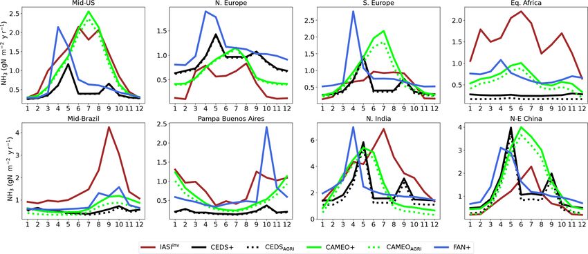
M. Beaudor et al.: Global agricultural ammonia emissions simulated with ORCHIDEE                                                     1059

Table 3. Emission factors (EFs) given as a percentage of the TAN content in the manure. EFs for the yard and the other N species come from
EMEP/EEA (2019). The other EFs are taken from Sommer et al. (2019). There is no distinction between liquid and solid manure for yard
EFs. Numbers in parentheses are the standard deviations given in Sommer et al. (2019) and used for the sensitivity analysis.

                        Manure type    EFNH3 (house)     EFNH3 (yard)    EFNH3 (store)   EFN2 (store)   EFNO (store)    EFN2 O (store)
    Dairy cattle        Liquid               19 (5.7)              30        25 (11.2)            0.3           0.01                0
    Dairy cattle        Solid                 8 (5.7)              30        32 (15.8)             30              1                2
    Non-dairy cattle    Liquid               19 (5.7)              53        25 (11.2)            0.3           0.01                0
    Non-dairy cattle    Solid                 8 (5.7)              53        32 (15.8)             30              1                2
    Pigs                Liquid              27 (12.1)               0         11 (6.9)            0.3           0.01                0
    Pigs                Solid               23 (12.6)               0        29 (15.6)             30              1                1
    Chickens            Solid               21 (11.5)               0        19 (15.9)             30              1              0.2
    Small ruminants     Solid                22 (5.7)              75        30 (15.8)             30              1                2

   The remaining manure after storage m(applic,a) and the ma-                grassland PFTs receive stored manure with a 2 times
nure produced during grazing m(graz,a) are the main output                   higher preference for cropland fractions.
of this specific module. Both quantities are the input for the
surface application component of the model (described in the
next section).

Organic application onto land

This section contains the description of the manure applica-              – Manure deposited during grazing activity by the rumi-
tion to soil. m(applic,a) and m(graz,a) are the manure remain-              nants. The manure from grazing activity m(graz,a) is cal-
ing after storage and the manure produced during grazing,                   culated in Eq. (7) and is assumed to be only deposited
respectively (a description is given in Sect. 2.1). Both are                on grassland PFTs by ruminants. The first day of ma-
yearly stocks applied daily at a constant rate and during a                 nure deposition for grazing also corresponds to the be-
specific period, driven mainly by environmental conditions,                 ginning of vegetation growth. The amount and period
as described below. This assumption may neglect the actual                  of manure deposited during grazing are animal-specific
seasonal patterns of N application usually defined by local                 and are determined by the fraction of time passed graz-
governance in some regions. For instance, as discussed in                   ing (xgraz,a ).
Van Damme et al. (2022), the time of the year when fertiliz-
ers can be applied in Europe is strongly dependent on local
regulations. Synthetic fertilizers are also considered in our
representation and follow the same temporal distribution as
the manure from storage. Note that ORCHIDEE does not dif-               The soil–plant–atmosphere processes leading to soil
ferentiate between natural and managed grassland. Only grid             emissions
cells with either the presence of livestock or fertilizer appli-
cation are considered for the emission calculation, so we can
assume that the pixel is managed.                                       In this section, we describe the physical processes in the soil
   As previously stated, the following two types of manure              that influence ammonia emissions. A single soil TAN pool
are considered:                                                         (TAN(soil) , g N m−2 ) is considered. The soil TAN pool is dy-
                                                                        namically updated depending on the processes implemented
  – Manure from storage and applied to soil as fertilizer.              in the model. These processes are described in Zaehle and
    The manure from storage is applied daily at a con-                  Friend (2010). The processes corresponding to the creation
    stant rate for 6 months from the beginning of vegeta-               of NH+ 4 are related to mineralization, N application, and NHx
    tion growth, corresponding to the first leaf development            deposition, whereas the losses include nitrification, leaching,
    depending on the PFT. The intermediate period of appli-             and volatilization.
    cation (Lapplication = 6 months) has been chosen in order              TAN(soil,aq) corresponds to the ammonium pool TAN(soil) ,
    to account for the heterogeneity in the agricultural prac-          which is assumed to be diluted in the soil water at a different
    tices, as the model only represents C3 and C4 crop types            heights in the soil according to the zactivity parameter.
    within the grid cell. Moreover, there is a lack of infor-              The zactivity parameter is regulated by all TAN sources,
    mation in the literature about N application onto grass-            called “input” (“min” – mineralization, “dep” – deposition,
    land at the global scale. We assume that cropland and               BNF, “fert” – mineral fertilizer, and “manure” – applied ma-

https://doi.org/10.5194/gmd-16-1053-2023                                                   Geosci. Model Dev., 16, 1053–1081, 2023
1060                                   M. Beaudor et al.: Global agricultural ammonia emissions simulated with ORCHIDEE

Table 4. Summary of the data sources used in Sects. 2.1 and 2.1 for the calculation of the indoor emissions. All of the data are used for each
livestock type a except for the Ddairy cattle,i variable.

     Abbreviation                        Description                                      Unit                    Sources
     D                                   Spatial distribution for 2006                    head km−2               Robinson et al. (2014)
     Ddairy cattle,i                     Country level i annual dairy cattle stocks       head                    FAOSTAT (2020)
     W                                   Regional typical animal weight                   kg                      Adapted from FAO (2018)
     dcrop/grass                         Regional diet composition                        %                       Adapted from FAO (2018)
     Straw                               Annual straw used in bedding                     kg FM head−1 yr−1       EMEP/EEA (2019)
     Nretention frac                     N-retention fraction                             %                       Paustian et al. (2006)
     Lhousing                            Housing period                                   day                     EMEP/EEA (2019)
     xTAN                                Fraction of TAN in N excreted                    %                       EMEP/EEA (2019)
     xliq                                Regional manure types                            %                       Adapted from FAO (2018)
     EFN2 O (stor) , EFN2 (stor) ,       European EFs.                                    % TAN                   EMEP/EEA (2019)
     EFNO (stor) , EFNH3 (small rum)     Every EF for small ruminants
     EFNH3 (indoor)                      NH3 European EFs                                 % TAN                   Sommer et al. (2019)

nure and manure from grazing), in soil as follows:                           The emissions of NH3 (ENH3 , g N m−2 s−1 ) are obtained
                                                                          following the resistive scheme used in the FAN model (Rid-
zactivity (t) =(pzact_deep
                                                                          dick et al., 2016; Vira et al., 2020):
              × inputmin + pzact_deep × inputdep
                                                                                      NH3 (g) − χa
              + pzact_deep × inputbnf +                                   ENH3 =                   ,                                        (16)
                                                                                       Ra (z) + Rb
              pzact_surf (fert) × inputfert
              + pzact_surf (manure)                                       where NH3 (g) is the NH3 concentration at the sur-
                                                                          face (g N m−3 ), χa is the free-atmosphere concentration
              × inputmanure + zactivity (t − 1)
                                                                          (g N m−3 ), Ra (z) is the aerodynamical resistance (s m−1 ),
              × TAN(soil) )                                               and Rb is the quasi-boundary-layer resistance (s m−1 ).
                          1                                                  χa is prescribed as a monthly field averaged over 11 years
              ×                      ,                          (13)
                inputtot + TAN(soil)                                      from a run of the global LMDZ-INCA (Laboratoire de
                                                                          Météorologie Dynamique–INteraction with Chemistry and
where inputtot denotes the total TAN sources in soil. We as-
                                                                          Aerosols) model at a 2.5◦ × 1.3◦ resolution (39 vertical lev-
sume that the fertilization and the application of manure are
                                                                          els) over the 2005–2015 period (Hauglustaine et al., 2014).
surface N additions to soil, whereas the other sources of TAN
                                                                          The spatial distribution of χa is presented in Fig. S4 (Sup-
(mineralization, deposition, and BNF) are deeply added into
                                                                          plement) for both May and December (2005–2015 climatol-
soil (pzact_deep = 1.0 m). It is worth noting that inputfert is
                                                                          ogy).
given as the ammonium content of the total N mineral fertil-
                                                                             Ra (z) is computed interactively by the biophysics module
izer applied (the parameter FracNH+ ,fert is the fraction of the
                                     4                                    of the ORCHIDEE model. Rb has been implemented accord-
ammonium content of the N fertilizer used to make the con-                ing to Xu et al. (2019) as follows:
version, and this parameter is tested in the sensitivity analy-
sis).                                                                                 v

                                                                                                       c

                                                                                                                l × µ∗ 1/3

   pzact_surf is obtained as described in Riddick et al. (2016):          Rb =              ×               ×              ,                (17)
                                                                                 DNH3                (LAI)2        v
pzact_surf(manure) = sW (m) × inputmanure /SWC,
                                                                          where DNH3 is the molecular diffusivity of NH3 in air
pzact_surf(fert) = sW (f ) × inputfert /SWC.                    (14)      (m2 s−1 ; Massman, 1998), c is an empirical constant equal
Here, SWC is the soil water content computed by OR-                       to 3, l is the leaf width (0.02 m; Massad et al., 2010),
CHIDEE, sW (m) is the specific water volume of manure                     v is the kinematic viscosity of air (1.56 × 10⁻⁵ m2 s−1 at
(5.67 × 10⁻⁴ m3 of water per gram of nitrogen; Sommer and                 25 ◦ C), T is the air temperature (in K), and LAI is the leaf
Hutchings, 2001; Riddick et al., 2016), and sW (f ) is the spe-           area index (m2 m−2 ), which is computed by the ORCHIDEE
cific water volume of synthetic fertilizers. sW (f ) depends on           model. The resulting annual mean Rb ranges between 0 and
the soil temperature Tg and is given by United Nations In-                1.14 s m−1 over the globe. DNH3 is a function of temperature
dustrial Development Organization (UNIDO):                                and is written as follows:
                                                                                                       1.81
                         1 × 10⁻⁶

                                                                                                   T
SW (f ) =                                       .               (15)      DNH3 = 0.1978 ×                    × 10−4 .             (18)
            0.466 × 0.66 × e0.0239×(Tg −273)                                                    273.13

Geosci. Model Dev., 16, 1053–1081, 2023                                                          https://doi.org/10.5194/gmd-16-1053-2023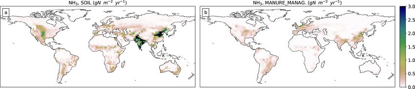
M. Beaudor et al.: Global agricultural ammonia emissions simulated with ORCHIDEE                                             1061

   Henry’s law coefficient (KH ) and the dissociation con-         reasonable computing cost. We also performed a reference
stant of NH+4 (aq) in water (KNH4 ) (Sutton et al., 1994) are      simulation at a 0.5◦ resolution to ensure that the model res-
used for the speciation between the different  TAN species         olution does not affect the results. We performed a 10-year
(NH3 (g), NH3 (aq), NH+             −3 ).

                        4 (aq) g N m                               reference simulation over the 2005–2015 period. This sim-
                                                                 ulation starts in January 2005 from a simulation done with
        NH3 (aq)                                                   an ORCHIDEE version similar to the one presented in this
KH =                                                    (19)
                                                                   paper but without the developments presented in Sect. 2.1.2.

         NH3 (g)
          +                                                    In the reference simulation, all annual forcing data are up-
          H     NH3 (aq)
KNH4 =  +                                              (20)      dated every year except those related to BNF and the live-
             NH4 (aq)                                              stock density, which are constant over time. A set of nine
                                                                   sensitivity test simulations characterized by specific changes
By combining Eqs. (19) and (20), we can compute the
                                                                   in the parametrization were conducted to evaluate the impact
gaseous phase of ammonia NH3 (g), which is the fraction that
                                                                   of parameter uncertainty on agricultural ammonia emissions.
will be volatilized. TAN(soil,aq) corresponds to the aqueous
                                                                   The parameters that have been tested are the atmospheric am-
phase of TAN in the soil, which is modulated by the height
                                                                   monia concentration (χa ), the pH of the manure (pH, default
of the soil through the zactivity parameter.
                                                                   value of 7), the timing period of N application (Lapplication ,
            TAN(soil,aq)                                           default value of 183 d), the emission factor for housing and
NH3 (g) =      θ
                           ,                               (21)    storage activities (EFNH3 (indoor) ), the fraction of ammonium
              Kfact   +
                                                                   in fertilizer (FracNH+ ,fert , default value of 0.6), and the N
                                                                                          4
where θ is the volumetric soil water content (in cubic meters      deep processes regulation parameter (pzact_deep , default value
of water per cubic meter of soil), and  is the fraction of the    of 1 m). Table 5 summarizes the set of simulations and the
air-filled soil volume computed by the ORCHIDEE model.             key parameters tested.
   Kfact is calculated as                                             In Riddick et al. (2016), the value of χa was set to
                                                                   0.3 µg N m−3 , as it is representative of the concentration over
Kfact = 1/(1 + KH + KH H+ /KNH4 ),

                                                          (22)     low-activity agricultural sites (Zbieranowski and Aherne,
                                                                   2012). Little sensitivity of the emissions to this parameter
and KH , Henry’s law constant for NH(3) , depends on the sur-      was found because χa is much smaller than NH3 (g). How-
face temperature Tg as follows:                                    ever, this parameter has been tested in our implementation
                                                                   through a sensitivity analysis.
KH = H × Tg × e4092(1/Tg −1/Tref ) ,                       (23)       The ORCHIDEE model requires the following set of forc-
                                                                   ing data:
where Tref is the reference temperature (298.15 K), and H
is a conversion factor equal to 4.905. We use the value of           – meteorological data, including the near-surface air tem-
0.59 mol m−3 Pa−1 described in Sander (2015) by which the              perature and specific humidity, wind speed, pressure,
perfect gas constant has been multiplied in order to get a unit-       short- and long-wave incoming radiation, rainfall, and
less constant. KNH4 is the dissociation equilibrium and also           snowfall, from the Climatic Research Unit (CRU) and
depends on the surface temperature Tg as follows:                      Japanese reanalysis (JRA) dataset (CRU-JRA V2.1)
                                                                       (Harris et al., 2014) (preprocessed and adapted by
KNH4 = 5.67 × 10⁻¹⁰ × e−6286(1/Tg −1/Tref ) .              (24)        Vladislav Bastrikov, LSCE, July 2020), provided at 6 h
                                       +
   The hydrogen ion concentration H is assumed to be                   time steps;
constant and equal to 10−7 , which approximately corre-              – the global average annual atmospheric CO2 concentra-
sponds to the pH given in Massad et al. (2010) for cattle ma-          tion, which is provided by TRENDY (Le Quéré et al.,
nure, diammonium phosphate fertilizers in acidic soils, and            2018);
ammonium nitrate fertilizers. A pH of 7 is also adopted in
Riddick et al. (2016). In our simulations, the pH does not im-       – the global annual land cover distribution, based on com-
pact the surrounding soil pH in the model, in contrast to Vira         bined information from the Land-Use Harmonization
et al. (2020), where the pH varies according to different TAN          2 (LUH2v2) dataset at a 0.25◦ resolution (Hurtt et al.,
age classes.                                                           2020) and the ESA (2022) CCI Land Cover (see Lurton
                                                                       et al., 2020, for more details);
2.2   Modeling setup
                                                                     – atmospheric N deposition fluxes (NHx and NOy ) from
The ORCHIDEE model, including all of the developments                  the IGAC/SPARC Chemistry-Climate Model Initiative
described in Sect. 2, was run at a spatial resolution of 2◦            (CCMI; Eyring et al., 2013), which have been used in
(180 × 90). This spatial resolution is relatively low but en-          the N2 O Model Intercomparison Project (NMIP) project
ables one to perform an ensemble of sensitivity tests at a             (Tian et al., 2018), corresponding to information at a

https://doi.org/10.5194/gmd-16-1053-2023                                             Geosci. Model Dev., 16, 1053–1081, 2023
1062                                M. Beaudor et al.: Global agricultural ammonia emissions simulated with ORCHIDEE

Table 5. Summary of the simulations performed and the parameters tested. The EFNH3 (indoor) parameter is described in Sect. 2.1 for housing
and storage emissions. The equations and sections related to the individual parameters are also indicated.

             Simulation       Parameter tested   Value                                                 Equation or section
             CONC0.3          χa                 0.3 µgNm−3                                            Eq. (16)
             CONC3            χa                 3 µgNm−3                                              Eq. (16)
             pH7.5            pH                 7.5                                                   Eq. (22)
             TIM10            Lapplication       10 d                                                  Sect. 2.1
             TIM365           Lapplication       365 d                                                 Sect. 2.1
             EFmax            EFNH3 (indoor)     (reference value + standard deviation); see Table 3   Eqs. (8), (9), and (12)
             FERT0.75         FracNH+ ,fert      0.75                                                  Eqs. (13) and (14)
                                     4
             pzact_deep,1.5   pzact_deep         1.5 m                                                 Eq. (13)

      0.5◦ spatial resolution and a monthly temporal resolu-            because our work is based on a similar approach. The re-
      tion;                                                             gional budget accounts for Africa; tropical southern Asia;
                                                                        Europe; China, Korea, and Japan (abbreviated as China–K–
  – the annual mineral fertilizer rates over croplands and              J in the figures); Oceania; India; the USA and Canada; and
    grasslands from an annual dataset developed by Lu                   Latin America. The seasonal variations in ammonia emis-
    and Tian (2017), which corresponds to a reconstruction              sions are also evaluated against satellite-derived emissions
    from 1960 to 2014 for the global cropland matched with              (Evangeliou et al., 2020). For that purpose, atmospheric NH3
    the HYDE 3.2 cropland distribution;                                 columns observed by the Infrared Atmospheric Sounding In-
                                                                        terferometer (IASI) satellite have been combined with the
  – the biological nitrogen fixation rate, which is provided            NH3 lifetime calculated by LMDZ-INCA in order to re-
    as climatological data as a function of the evapotranspi-           trieve emissions. The NH3 retrieval product used to derive
    ration flux (see Vuichard et al., 2019, for more details);          emissions in our study comprises the 2011–2015 morning
                                                                        observations (Metop-A and -B) and follows a neural net-
  – the distribution of each livestock category, which is               work retrieval approach (ANNI-NH3-v3R), as referred to in
    taken from the Gridded Livestock of the World (GLW                  Van Damme et al. (2017, 2021). Both the lifetime and at-
    2; Robinson et al., 2014) and represents the gridded an-            mospheric columns are monthly products and share the ex-
    imal densities (Da ) for the year 2006 at a 1 km resolu-            act same grid resolution (LMDZ-INCA grid resolution at
    tion. Small-ruminant densities correspond to the sum of             2.5◦ ×1.3◦ ). All three CAMEO, CEDS, and FANv2 seasonal
    the sheep and goat densities. The dairy cattle distribu-            variations are evaluated against IASI-derived emissions (de-
    tion has been retrieved from the total cattle distribution          fined as IASIinv ). In order to be consistent with IASI observa-
    combined with national dairy cattle densities given by              tions (where no source distinction is possible), the CAMEO,
    FAOSTAT (2020). The calculation adopted is described                CEDS, and FANv2 agricultural emissions need to be comple-
    in the Supplement.                                                  mented by fire emission data taken from van der Werf et al.
                                                                        (2017) (Global Fire Emissions Database, GFED s4) as well
2.3    Model evaluation dataset                                         as by industrial and waste sources (McDuffie et al., 2020).
                                                                        The extended emissions are referred to as CAMEO+ , FAN+ ,
Our integrated approach allows the computation of differ-               and CEDS+ , respectively, as described in Table 7. It is im-
ent variable levels before the final emission results, such as          portant to note that only the ORCHIDEE model can provide
biomass productivity, animal excretion rate, and manure pro-            natural emissions; this source is not considered in the FAN+
duction. This set of variables offers the advantage of evalu-           nor the CEDS+ datasets.
ating our emissions at different stages of the N flow against
the previous works listed in Table 6.
   The decadal mean (2005–2015) values of global and re-                3     Results and evaluation
gional calculated agricultural emissions, including indoor
and soil emissions, are compared to the CEDS inventory                  3.1    Evaluation of intermediate variables
(McDuffie et al., 2020) and the emissions simulated by
FANv2 (Vira et al., 2020). From the LMDZ–ORCHIDEE–                      Using the ORCHIDEE model, we estimate the total
INCA coupling development perspective, it is interesting to             biomass produced, including grass and crop, to be about
compare our approach with CEDS (McDuffie et al., 2020),                 103 Tg N yr−1 , which is slightly lower than previous esti-
as it is a reference dataset offering a long period of data             mates (110–152 Tg N yr−1 estimated by Bouwman et al.,
(1750–2019). FANv2 has been chosen for our evaluation                   2013a; Billen et al., 2014; Bodirsky et al., 2014; Conijn et al.,

Geosci. Model Dev., 16, 1053–1081, 2023                                                  https://doi.org/10.5194/gmd-16-1053-2023
M. Beaudor et al.: Global agricultural ammonia emissions simulated with ORCHIDEE 1063
Table 6. Summary of the different simulated variables evaluated in this work by comparison with previous studies.
Metric Description Unit Previous studies
BMharv/graz Global crop and grass production Tg N yr−1 Bouwman et al. (2013a);
Billen et al. (2014); Bodirsky et al. (2014);
Conijn et al. (2018); Uwizeye et al. (2020)
BMing,tot Global N intake by livestock Tg N yr−1 Billen et al. (2014); Bodirsky et al. (2014);
Conijn et al. (2018); Uwizeye et al. (2020)
ENH3 (indoor) NH3 emissions from housing, yarding, and storage kgN m−2 yr−1 Crippa et al. (2018); Vira et al. (2020)
mN,excr/applic Global amount of manure excreted/applied Tg N yr−1 Beusen et al. (2008); Potter et al. (2010);
Bouwman et al. (2013b); Billen et al. (2014);
Bodirsky et al. (2014); Zhang et al. (2017a);
Conijn et al. (2018); Vira et al. (2020);
Uwizeye et al. (2020)
FN Global amount of fertilizer applied Tg N yr−1 Bouwman et al. (2013b); Billen et al. (2014);
Bodirsky et al. (2014); Zhang et al. (2017a);
Conijn et al. (2018); Vira et al. (2020);
Uwizeye et al. (2020)
ENH3 NH3 emissions from agriculture Tg N yr−1 McDuffie et al. (2020); Vira et al. (2020);
Evangeliou et al. (2020)
Table 7. Summary of the different datasets used in the comparison with the IASI-derived emissions. All of the emission sets (except FANv2
data, which are a 2010–2015 climatology) are taken from the 2011–2015 period and have been gridded onto the LMDZ-INCA default
resolution of 144 × 142 pixels.
Configuration Emission category Data sources
CAMEO+ Agricultural emissions ORCHIDEE run
Natural emissions ORCHIDEE run
Waste and industrial sources CEDS (McDuffie et al., 2020)
Biomass burning GFEDs4 (van der Werf et al., 2017)
FAN+ Agricultural emissions FANv2 data (2010–2015) (Vira et al., 2020)
Natural emissions Not taken into account in this dataset
Waste and industrial sources CEDS (McDuffie et al., 2020)
Biomass burning GFEDs4 (van der Werf et al., 2017)
CEDS+ Agricultural sources CEDS (McDuffie et al., 2020)
Natural emissions Not taken into account in this dataset
Waste and industrial sources CEDS (McDuffie et al., 2020)
Biomass burning GFEDs4 (van der Werf et al., 2017)
2018; Uwizeye et al., 2020). The calculated global annual tal biomass ingested by the livestock (88 Tg N yr−1 ) is lower
crop production (expressed in N) is about 74 Tg N yr−1 and than the range found in the literature (122–167 Tg N yr−1 ;
compares well with the 72 and 74 Tg N yr−1 estimated by Billen et al., 2014; Bodirsky et al., 2014; Conijn et al., 2018;
Billen et al. (2014) and Zhang et al. (2021), respectively. Uwizeye et al., 2020) which can be attributed to the low
The calculated annual grass production (28.8 Tg N yr−1 ) is grassland production calculated in our model.
more than 3 times lower than the 80.3 Tg N yr−1 reported by However, if the grass N production is largely underesti-
Billen et al. (2014) and estimated from the difference be- mated by ORCHIDEE, our grass C production estimate of
tween livestock ingestion and available feed resources. By 1.2 Pg C yr−1 is close to the value of 1.95 Pg C yr−1 reported
doing so, uncertainties from several components (crop pro- in the Fifth Assessment Report (AR5) of the IPCC (Smith
duction, net import of vegetal proteins, and human consump- et al., 2014). In this respect, an overestimation of the C : N
tion of vegetal proteins) are accumulated. Our resulting to- ratio may also explain part of the grass N production under-
https://doi.org/10.5194/gmd-16-1053-2023 Geosci. Model Dev., 16, 1053–1081, 20231064 M. Beaudor et al.: Global agricultural ammonia emissions simulated with ORCHIDEE
Table 8. Global estimates of intermediate variables computed by China, India, Africa, Latin America, the USA, and Europe
the model in this study for the 2005–2015 period and the range of appear as the main contributors to global NH3 emissions,
previous estimates. accounting for 80 % of the total budget (Fig. 3b). Most of
these source areas, which have also been identified as agri-
Metric This study Range of previous cultural regions by Van Damme et al. (2018), are regions
estimates with intensive crop cultivation (Fig. S2) and important live-
BMharv/graz (Tg N yr−1 ) 103 110–152 stock activities, inducing high N application rates (Fig. 2).
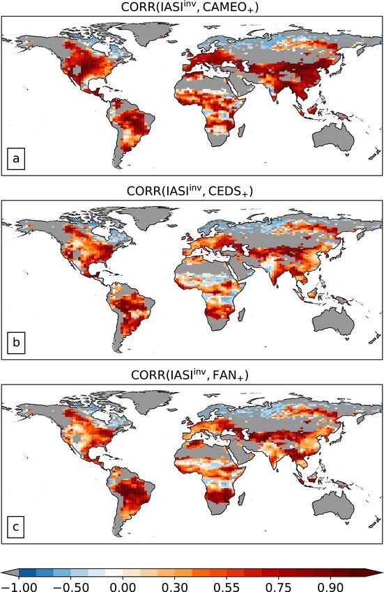
BMing,tot (Tg N yr−1 ) 88 122–167 The spatial distributions of the calculated agricultural NH3
mN,applic (Tg N yr−1 ) 66 32–131 emissions show good agreement with the FANv2 and CEDS
FN (Tg N yr−1 ) 121.6 55–116 results (Fig. 4, b, c). In India and China, our emissions are
slightly higher than FANv2 and CEDS estimates. Our val-
ues are lower than the FANv2 estimate in Latin America and
Africa but high compared with CEDS emissions, which are
estimation. It can be explained using a unique grass C : N particularly low in these two regions. In some parts of Africa
ratio per pixel and a global C : N ratio for crop in the model. and Latin America, where the use of synthetic fertilizer is
Because we assume that all of the manure stored is then ap- low (never exceeding 2500 kg N km−2 yr−1 ), livestock activ-
plied to soil, for the evaluation phase, we only consider data ity appears to be the main contributor to the emissions.
from the literature that estimate the application rate of ma- In intensive agricultural regions, data used for mineral
nure to soil. The global annual amount of manure application fertilizer application rates can be a source of discrepancy
(66 Tg N yr−1 ) is lower than the range of 99–129 Tg N yr−1 between models. Vira et al. (2020) use the LUH2 dataset
estimated in recent studies (Beusen et al., 2008; Potter et al., (Hurtt et al., 2020), which assumes that only croplands are
2010; Bouwman et al., 2013b; Billen et al., 2014; Zhang fertilized. The amounts of fertilizer applied over croplands
et al., 2017a; Conijn et al., 2018; Vira et al., 2020; Uwizeye are comparable globally between Vira et al. (2020) and our
et al., 2020). study (respective minimum–maximum of 79–87 and 96–
Figure 2 compares the distribution of the N manure ap- 101 Tg N yr−1 over 2010–2015) but differ in some regions
plied with the values retrieved by Zhang et al. (2017a) for the (see Fig. S2a). In addition, in our study, grasslands are also
year 2006 in order to be consistent with the reference live- fertilized with a global amount of 25.7 Tg Nyr−1 . This leads
stock distribution used in our approach. The spatial distribu- to differences in the simulated soil emissions, more specif-
tion of the manure application highlights the main livestock- ically in India, the USA, and China, where grasslands are
raising regions, such as China, India, Europe, Latin America, highly fertilized (Fig. S2b) and can be translated into high
and the USA. It shows good consistency with Zhang et al. volatilization rates when compared with FANv2.
(2017a), although it is higher in India, the USA, and Latin NH3 emissions peak in June–July–August for most re-
America and lower in China and Europe. These differences gions (the USA, Europe, China, and Africa; Fig. 5)
can be explained by the fact that we use different regional with maximum values reaching 16.4 g N m−2 yr−1 in east-
animal weights per livestock category (Table 1), instead of ern China. The peak in India appears earlier in spring,
a fixed value as in Zhang et al. (2017a). This induces dif- whereas two peaks occur in Latin America: one during
ferent N demands for similar livestock and, ultimately, dif- December–January–February and one during September–
ferent quantities of applied manure. Indeed, we use recently October–November. Depending on the region, the season-
adapted data for animal weights from FAO (2018), whereas ality of the emissions varies according to different factors,
Zhang et al. (2017a) used IPCC guidelines (Tier1 IPCC, including environmental parameters and agricultural prac-
2006; Paustian et al., 2006). For instance, for India, the non- tices. This aspect will be analyzed in more detail in Sect. 3.4
dairy cattle weight is almost 4 times higher, which explains and 3.5.
the differences observed in our calculation. Moreover, our The spatial pattern of the simulated indoor NH3 emissions
study assumes a unique N excretion rate per livestock type (Fig. 6b) is similar to that of manure application rates, with
and no livestock system distinctions as a simplification. both being driven mainly by livestock density. Hot spot re-
gions of indoor emissions are located in eastern China, east-
3.2 Agricultural emissions at the global scale ern India, and northern Europe, with maximum values reach-
ing up to 1.7 g N m−2 yr−1 . The major sources of volatiliza-
We estimate global NH3 agricultural emissions (averaged tion from soils are located in India, eastern China, and the
over 2005–2015) of about 44 Tg N yr−1 : 78 % from soil USA, with a maximum value of 12 g N m−2 yr−1 . The differ-
volatilization (driven by fertilizer and manure application) ence in spatial patterns between the two source categories is
and the remainder from indoor emissions (from livestock mainly due to the fact that soil emissions not only depend
housing, yarding, and storage). These global NH3 emissions on livestock distribution (indoor emissions) but also on envi-
are within the range given by McDuffie et al. (2020) and Vira ronmental conditions and mineral fertilizer application rates.
et al. (2020) of 39–47 Tg N yr−1 (Fig. 3a).
Geosci. Model Dev., 16, 1053–1081, 2023 https://doi.org/10.5194/gmd-16-1053-2023You can also read