Last Glacial Maximum to Holocene paleoceanography of the northwestern Ross Sea inferred from sediment core geochemistry and micropaleontology at ...
←
→
Page content transcription
If your browser does not render page correctly, please read the page content below
J. Micropalaeontology, 40, 15–35, 2021
https://doi.org/10.5194/jm-40-15-2021
© Author(s) 2021. This work is distributed under
the Creative Commons Attribution 4.0 License.

       Last Glacial Maximum to Holocene paleoceanography of
       the northwestern Ross Sea inferred from sediment core
        geochemistry and micropaleontology at Hallett Ridge
           Romana Melis1 , Lucilla Capotondi2 , Fiorenza Torricella3 , Patrizia Ferretti4 , Andrea Geniram1 ,
             Jong Kuk Hong5 , Gerhard Kuhn6 , Boo-Keun Khim7 , Sookwan Kim5 , Elisa Malinverno8 ,
                                       Kyu Cheul Yoo5 , and Ester Colizza1
           1 Dipartimento   di Matematica e Geoscienze, Università di Trieste, Via E. Weiss 2, 34127 Trieste, Italy
                      2 Consiglio   Nazionale delle Ricerche–Istituto di Scienze Marine (CNR-ISMAR),
                                             Via Gobetti 101, 40129 Bologna, Italy
               3 Dipartimento di Scienze della Terra, Università di Pisa, Via Santa Maria 53, 56126 Pisa, Italy
                                 4 Dipartimento di Scienze Ambientali, Informatica e Statistica,

                              Università Ca’ Foscari, Via Torino 155, Mestre, 30172 Venice, Italy
                                 5 Korea Polar Research Institute, Incheon, 21990, South Korea
                        6 Alfred-Wegener-Institut Helmholtz Zentrum für Polar- und Meeresforschung,

                                      Am Alten Hafen 26, 27568 Bremerhaven, Germany
                   7 Department of Oceanography, Pusan National University, Busan, 46241, South Korea
                    8 Dipartimento di Scienze dell’Ambiente e della Terra, Università di Milano-Bicocca,

                                           Piazza della Scienza 4, 20126 Milan, Italy
                         Correspondence: Lucilla Capotondi (lucilla.capotondi@bo.ismar.cnr.it)

         Received: 15 September 2020 – Revised: 1 February 2021 – Accepted: 2 February 2021 – Published: 10 March 2021

      Abstract. During the Late Pleistocene–Holocene, the Ross Sea Ice Shelf exhibited strong spatial variability in
      relation to the atmospheric and oceanographic climatic variations. Despite being thoroughly investigated, the
      timing of the ice sheet retreat from the outer continental shelf since the Last Glacial Maximum (LGM) still
      remains controversial, mainly due to a lack of sediment cores with a robust chronostratigraphy. For this reason,
      the recent recovery of sediments containing a continuous occurrence of calcareous foraminifera provides the
      important opportunity to create a reliable age model and document the early deglacial phase in particular. Here
      we present a multiproxy study from a sediment core collected at the Hallett Ridge (1800 m of depth), where sig-
      nificant occurrences of calcareous planktonic and benthic foraminifera allow us to document the first evidence
      of the deglaciation after the LGM at about 20.2 ka. Our results suggest that the co-occurrence of large Neoglobo-
      quadrina pachyderma tests and abundant juvenile forms reflects the beginning of open-water conditions and
      coverage of seasonal sea ice. Our multiproxy approach based on diatoms, silicoflagellates, carbon and oxygen
      stable isotopes on N. pachyderma, sediment texture, and geochemistry indicates that abrupt warming occurred
      at approximately 17.8 ka, followed by a period of increasing biological productivity. During the Holocene, the
      exclusive dominance of agglutinated benthic foraminifera suggests that dissolution was the main controlling fac-
      tor on calcareous test accumulation and preservation. Diatoms and silicoflagellates show that ocean conditions
      were variable during the middle Holocene and the beginning of the Neoglacial period at around 4 ka. In the
      Neoglacial, an increase in sand content testifies to a strengthening of bottom-water currents, supported by an
      increase in the abundance of the tycopelagic fossil diatom Paralia sulcata transported from the coastal regions,
      while an increase in ice-rafted debris suggests more glacial transport by icebergs.

Published by Copernicus Publications on behalf of The Micropalaeontological Society.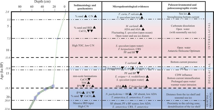
16                                                       R. Melis et al.: Last Glacial Maximum to Holocene paleoceanography

1    Introduction                                                      Ross Sea ice sheet–shelf dynamics were principally inves-
                                                                    tigated in the continental shelf via geophysical and geolog-
Ice shelves are very sensitive to climatic variations, with         ical methods (Domack et al., 1999; Anderson et al., 2014;
their dynamics being related to the atmospheric and ocean           Prothro et al., 2018, 2020; Smith et al., 2019). The typi-
warming–cooling causing changes in the accumulation and             cal sedimentary succession from sub-glacial diamicton to-
discharge of upstream glacial ice. The Ross Sea Ice Shelf,          ward proximal to distal deglacial glaciomarine sediments and
the largest in Antarctica, has been investigated over recent        Holocene open marine diatom-bearing mud, recording a pro-
decades as it drains parts of the two main ice sheets, the          gressive retreat of the ice sheet–shelf and the final onset of
West Antarctic Ice Sheet (WAIS) and the East Antarctic Ice          seasonal open marine conditions, has been well-documented
Sheet (EAIS), which extended toward the outer continental           (Prothro et al., 2018, 2020; Smith et al., 2019). In this study
margin during the Last Glacial Maximum (LGM) (Ander-                we extend the investigations to the outer continental shelf–
son et al., 2014, 2018; Halberstadt et al., 2016; Simkins et        slope system, which is more complex and still scarcely in-
al., 2017). Even though the time and mode of the retreat            vestigated (Quaia and Cespuglio, 2000; Bonaccorsi et al.,
of these ice sheets since the LGM have been extensively             2007; Tolotti et al., 2013; Frank et al., 2014). The sedimenta-
studied and new models have recently been presented (e.g.,          tion of the continental slopes is strongly influenced by the
Golledge et al., 2014; Lowry et al., 2019), some controver-         dominant oceanographic processes and, in some cases, by
sies still remain due to the difficulties in obtaining accurate     the downward transport of sediment through the gravitational
radiocarbon dates. Published radiocarbon ages are predom-           sediment flow, which includes collapse, turbidity, and debris
inantly based on acid-insoluble organic matter (AIOM) ex-           flows (Jacobs, 1989). Moreover, based on the radiocarbon
tracted from bulk sediments (Livingstone et al., 2012; An-          dating performed on Neogloboquadrina pachyderma, we try
derson et al., 2014; Prothro et al., 2020). Indeed, the ages        to link and test models of the glacial retreat history.
obtained through these methods are frequently anomalously
old, with an overestimated age of glacial retreat (e.g., An-
drews et al., 1999; Hillenbrand et al., 2009; Anderson et al.,      2   Study area
2014; Prothro et al., 2020). For this reason, the availability
of well-preserved calcareous material represents an excellent       The Hallett Ridge is a structural high bordering the west side
opportunity to construct a more accurate age model as evi-          of the Central Basin, a semi-closed basin located at the mouth
denced in investigations performed in the Ross Sea (Bart et         of the JOIDES Basin at the continental shelf break of the
al., 2018; Melis and Salvi, 2020; Prothro et al., 2020). In this    western Ross Sea (Fig. 1a). The multibeam bathymetry ac-
work we investigate a sedimentary interval found in a deep-         quired during the IBRV Araon expeditions ANA03B in 2013
sea core at the Hallett Ridge (northwestern Ross Sea) char-         and ANA05B in 2015 (Fig. 1b) shows some slope failures
acterized by the presence of rich and well-preserved calcare-       and bathymetric ridges that are contour-parallel elongated
ous foraminiferal assemblages. The recovery of sediments            along the eastern slope of Hallett Ridge (Kim, 2018). The si-
containing foraminifera in the Antarctic continental margin         multaneously acquired sub-bottom profiler (SBP) data show
represents a good opportunity for paleoenvironmental studies        that acoustically stratified facies developed in the slope fail-
lacking the continuous presence of biogenic calcium carbon-         ure area (Fig. 1c), while relatively weak subsurface reflec-
ate. In the Southern Ocean, the occurrence of foraminifera is       tions are observed below high-amplitude seafloor reflection
strongly controlled by water-mass characteristics, which de-        on the contour-parallel mounds of the eastern slope of Hallett
termine the solubility of CaCO3 on the seafloor (e.g., Murray       Ridge (Kim, 2018). This provides indirect evidence that less
and Pudsey, 2004; Hauck et al., 2012; Dejong et al., 2015).         compacted and/or finer-grained sediment in the slope failure
However, their occurrence and distribution are very useful          area is relatively thicker than the bathymetric highs.
to characterize the lithofacies associated with glacial retreat        The studied area is influenced by dense and salty High-
patterns (e.g., Bart et al., 2016; Majewski et al., 2018; Prothro   Salinity Shelf Water (HSSW) coming from the mouth of the
et al., 2018, 2020). In this study, using integrated proxies,       JOIDES Basin. This water mass exported from the continen-
we provide new information on paleoceanographic condi-              tal shelf mixes with Circumpolar Deep Water (CDW) as it
tions in order to reconstruct the paleoenvironmental changes        descends the continental slope, producing Antarctic Bottom
in the Hallett Ridge area since Marine Isotope Stage (MIS)          Water (AABW) (Budillon et al., 2011; Castagno et al., 2019).
2. Our results, including benthic foraminifera, diatoms, and        AABW plays a key role in the thermohaline circulation in the
silicoflagellates, are used to better define paleoenvironmental     global climate system (Jacobs, 2004; Colleoni et al., 2018;
and paleoceanographic conditions. These microfossil groups          Tinto et al., 2019). On the other hand, the Central Basin rep-
are well-known as useful proxies for reconstructing the pa-         resents one of the preferred pathways for warm CDW flowing
leoenvironmental settings recorded in the sedimentary se-           onto the continental shelf (Dinniman et al., 2011) as modified
quence deposited in diverse facies related to an ice shelf–         CDW (mCDW) providing the main source of heat and nutri-
sheet from sub-glacial to open marine conditions (e.g., Smith       ents (Smith et al., 2012; Stevens et al., 2020) to the Ross Sea
et al., 2019, and references herein).                               continental shelf. Considering that this area has been most af-

J. Micropalaeontology, 40, 15–35, 2021                                                   https://doi.org/10.5194/jm-40-15-2021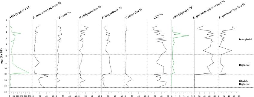
R. Melis et al.: Last Glacial Maximum to Holocene paleoceanography 17
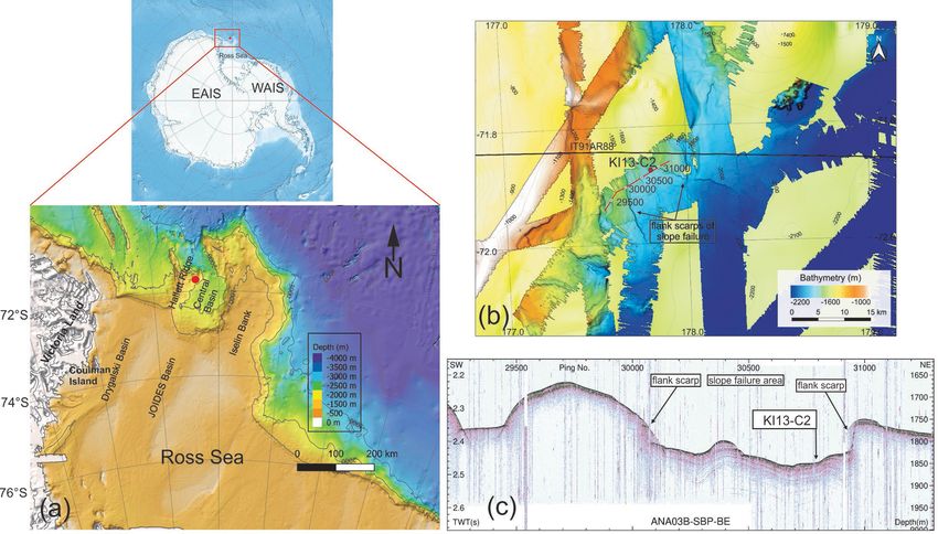
Figure 1. (a) Bathymetric map of the northwestern Ross Sea (modified from Arndt et al., 2013) and location of the KI13-C2 core (red
dot). (b) Multibeam bathymetry imagery of the study area and core location. The black line indicates the multi-channel seismic (MCS) line
IT91AR88. The red line and white dots represent the sub-bottom profile (SBP) data of ANA03B-SBP-BE, and labels refer to intervals of 500
ping numbers illustrated in the (c) SBP of ANA03B-SBP-BE and the core location. The Antarctica relief location map is from Wikimedia
Commons contributors.
fected by the contributions of the EAIS (Farmer et al., 2006; 3.1 Sedimentary analyses
Anderson et al., 2014), the sedimentary sequences preserved
in the Central Basin are located in an ideal location to pro- For grain size analyses, 17 samples were treated with hydro-
vide important information about the HSSW dynamics and gen peroxide to remove organic matter and sieved to sepa-
the EAIS evolution during the Quaternary glacial and inter- rate the < 2 mm fraction. Carbonate was removed with acetic
glacial cycles. acid in all samples with carbonate content > 5 %, in agree-
ment with McCave et al. (1995). The grain size of the <
2 mm size fraction was determined using the Malvern Mas-
3 Material and methods tersizer Hydro2000S diffraction laser particle size analyzer
from the Department of Mathematics and Geosciences, Tri-
Gravity core KI13-C2 (71◦ 52.50 S, 177◦ 48.10 E; water depth
este. Sand and mud classes were determined using the Fried-
∼ 1800 m) was collected during the IBRV Araon expedition
man and Sanders (1978) grain size classification. Grain size
in February 2013 in the framework of a joint project be-
parameters were calculated using the Folk and Ward formu-
tween Italian and Korean researchers (PNRA/ROSSLOPE
las (Folk and Ward, 1957). The > 2 mm fraction was counted
and K-PORT Projects). The core (232 cm long) is located
separately.
in the northwestern side of the Central Basin near the right
flank of the Hallett Ridge. Based on the SBP and multibeam
data acquired during the ANA03B expedition, the core was 3.2 Chronology
collected in the trough between the small contour-parallel
mounds (Fig. 1c), indicating that this area was affected by The chronology of the studied core is based on nine ac-
along-slope bottom current activity. Here we report data from celerator mass spectrometry (AMS) radiocarbon dates ob-
the upper 60 cm of sedimentary interval in which an abundant tained at the Poznań Radiocarbon Laboratory located at
presence of calcareous foraminifers has been recorded. Adam Mickiewicz University (Poland) and with the MI-
CADAS (Wacker et al., 2013) at the Alfred-Wegener-Institut
Helmholtz-Zentrum für Polar- und Meeresforschung (AWI,
https://doi.org/10.5194/jm-40-15-2021 J. Micropalaeontology, 40, 15–35, 2021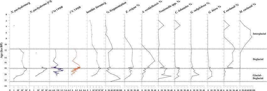
18                                                      R. Melis et al.: Last Glacial Maximum to Holocene paleoceanography

Germany). Five radiocarbon analyses were made using acid-
insoluble organic matter (AIOM), and four were carried out
on N. pachyderma tests (Table 1).
   Considering the different carbonate and organic carbon
matrices, we decided to directly calibrate the carbonate dates
and to treat AIOM dates prior to the calibration of 14 C ages.
Radiocarbon chronologies using the AIOM fraction from
bulk sediments are often compromised by contamination
from reworked ancient organic carbon derived from glacial
erosion and/or from the reworking of unconsolidated sedi-
ments (see Mezgec et al., 2017; Tesi et al., 2020, for a discus-
sion). This is evidenced by AIOM dates of Antarctic surface
sediments that extend over several thousand years (Andrews
et al., 1999; Pudsey et al., 2006).
   The down-core AIOM dates were corrected by the AIOM
age of the preserved core-top sediments of the box core
KI13-BC3, which was collected at the same site. We as-
sumed that the age difference between the AIOM 14 C age            Figure 2. (a) Age–depth model based on the linear interpolation
of the box-core and core-top sediment, along with the ma-          of best point calibration ages from AMS 14 C dates obtained using
rine reservoir effect (MRE), represents local contamination        Clam software (Blaauw, 2010). The dotted lines show the 95 % con-
with older organic matter in this area, and hereafter it is re-    fidence intervals based on 1000 iterations. (b) Sedimentation rate in
ferred to as “local contamination offset” (LCO; see the dis-       millimeters per year.
cussion in Hillenbrand et al., 2009). Before calibrating the
14 C dates, the LCO obtained for this area was subtracted

from the AIOM 14 C down-core ages (LCO-corrected ages),            than ±0.1 %. TOC content was calculated by the difference
assuming that both MRE and LCO did not change over the             between TC and TIC.
Holocene (see Hall et al., 2010; Mezgec et al., 2017, for de-
tails). We used an MRE of 1.1 ± 0.12 ka 14 C suggested by          3.3.2   Stable oxygen and carbon isotopes on planktic
Hall et al. (2010) for the Ross Sea area carbonate samples.                foraminifera
   The LCO-corrected AMS 14 C dates obtained for AIOM
                                                                   Stable oxygen and carbon isotope measurements were car-
and N. pachyderma tests were converted into calibrated ages
                                                                   ried out at 1 cm resolution on 39 samples (from 18 to
by means of Clam 2.3.2 (Blaauw, 2010) at 95 % confidence
                                                                   56 cm) using the planktic foraminifera Neogloboquadrina
ranges. The Marine13 calibration curve (Reimer et al., 2013),
                                                                   pachyderma. At least 20 adult specimens picked from the
assuming a regional marine offset (1R) of 0.79 ± 0.12 ka
                                                                   > 250 µm sediment size fraction were used for the analy-
from the global MRE (Hall et al., 2010), was used. CLAM
                                                                   sis in order to provide significant carbon dioxide. Specimens
2.3.2 (Blaauw, 2010) was also used to calculate the age–
                                                                   were lightly crushed and soaked in 1 % hydrogen peroxide
depth model through a linear interpolation function between
                                                                   for 30 min in individual vials in order to remove any possi-
dated levels with 1000 iterations (Fig. 2). Uncorrected and
                                                                   ble organic contaminant. Analytical-grade acetone was then
calibrated 14 C data are summarized in Table 1; all the ages re-
                                                                   added, and samples were cleaned ultrasonically for 30 s to re-
ported in this paper represent the calibrated ages unless oth-
                                                                   move fine-grained particles, after which the excess liquid and
erwise specified.
                                                                   residue were siphoned off. Samples were finally oven-dried
                                                                   overnight at 50 ◦ C before the analysis. Stable isotope analy-
3.3     Geochemical analyses                                       ses were carried out on VG SIRA mass spectrometer coupled
                                                                   with a Micromass Multicarb sample preparation system and
3.3.1    Sediment geochemistry                                     a Thermo Finnigan MAT253 mass spectrometer fitted with
                                                                   a Kiel device. Measurements of δ 18 O and δ 13 C were deter-
Total inorganic carbon (TIC) content was measured on 33
                                                                   mined relative to the Vienna Peedee Belemnite (VPDB) stan-
levels every 2 cm using a UIC CO2 coulometer (model
                                                                   dard, and the analytical precision was better than 0.08 ‰ for
CM5014) at Pusan National University (Korea). TIC content
                                                                   δ 18 O and 0.06 ‰ for δ 13 C. All isotope measurements were
was used to calculate the CaCO3 content as a weighted per-
                                                                   performed at the Godwin Laboratory for Palaeoclimate Re-
centage by the multiplication of factor 8.333 (CaCO3 / C ra-
                                                                   search, Department of Earth Sciences, University of Cam-
tio). The analytical precision of CaCO3 content as a relative
                                                                   bridge (UK).
standard deviation is ±1 %. The total carbon (TC) content of
the same sediment samples was measured by Flash 2000 Se-
ries elemental analyzer. The analytical precision of TC is less

J. Micropalaeontology, 40, 15–35, 2021                                                    https://doi.org/10.5194/jm-40-15-2021
R. Melis et al.: Last Glacial Maximum to Holocene paleoceanography                                                                                                         19

Table 1. AMS 14 C ages with calibrated calendar ages ±2σ (years) as well as applied local contamination offset and reservoir age correction
(see text) of the studied core. The calendar ages were calibrated using the Clam 2.3.2 software with a Marine13 calibration curve (Reimer et
al., 2013). A constant reservoir correction of 1144 ± 121 years with a 1R of 791 ± 121 years (Hall et al., 2010) was applied. Calibrated age
ranges are at 95 % confidence.

 Core and         Sample      Carbon       Lab                   Conventional        Error    LCOd          LCO         Median          Lower         Upper        Sedim.
 box core           depth     sourceb      no.c                      14 C age      (years)              corr. age    probability     cal range     cal range          rate
 ID                  (cm)                                             (yr BP)                            (yr BP)         cal age       (yr BP)       (yr BP)    (mm yr−1 )
                                                                                                                        (yr BP)
 KI13-BC3a           0–1      AIOM         Poz-69634                     5050          40
 KI13-C2             0–1      AIOM         Poz no. 2-69635               7110          40      3950         3160           1998          1887         2108                  –
 KI13-C2           14–15      AIOM         Poz no. 2-69636              11 780         80      3950         7830           7535          7404         7666               0.03
 KI13-C2           22–23      N. pachy     AWI-4812.1.1                 15 710        143         –             –         17 669        17 317       18 020              0.01
 KI13-C2           36–37      N. pachy     Poz-75519                    16 230        100         –             –         18 262        17 995       18 528              0.24
 KI13-C2           48–49      N. pachy     Poz no. 2-75519              17 080         90         –             –         19 179        18 926       19432               0.13
 KI13-C2           54–55      N. pachy     AWI-4813.1.1                 17 930        166         –             –         20 188        19 775       20 601              0.06
 KI13-C2           92–93      AIOM         Poz-121684                   29 900        450      3950        25 950         28 856        27 879       29 833              0.04
a Box core. b AIOM: acid-insoluble organic matter; N.pachy: monospecific planktonic tests. c Poz: Poznań Radiocarbon Laboratory, Poland; AWI: Alfred-Wegener-Institut
Helmholtz-Zentrum für Polar- und Meeresforschung, Germany. d LCO: local contamination offset; see text for explanation.

3.4     Micropaleontological analyses                                                     scriptions. The number of broken and/or etched foraminifera
                                                                                          allowed us to calculate the percent of fragmentation for each
3.4.1     Foraminifera                                                                    level.

A total of 22 sediment samples (1 cm thick) collected on
                                                                                          3.4.2     Diatoms
average every 1, 2, and 4 cm, depending on the sedimenta-
tion rate, were investigated for foraminiferal analysis. The                              A total of 33 samples collected on average every 1, 2, and
samples were dried, weighed, and wet-sieved on a 63 µm                                    4 cm, depending on the sedimentation rate, were obtained
mesh. The whole fraction > 63 µm was investigated. In the                                 for diatom analyses. Diatom slide preparation followed the
carbonate-rich interval, the samples were split in order to ob-                           technique described by Rathburn et al. (1997). Diatom anal-
tain an aliquot containing approximately 300 planktic and                                 ysis was performed with a light microscope at 1000× mag-
benthic individuals. The density for both planktic and benthic                            nification; Zeiss (Immersol oil 518) immersion oil was used
foraminifera was expressed as the number of specimens per                                 to allow the observation. At least 300 diatom valves in each
gram of total dry sediment, hereinafter referred to as speci-                             sample were identified and counted following the counting
mens per gram.                                                                            method outlined by Crosta and Koç (2007). The relative
    Following the ecology requirements of N. pachyderma, we                               abundance was determined for each taxon as the ratio be-
differentiated between encrusted (adults) and non-encrusted                               tween the diatom species and the total diatom abundance.
(juveniles) specimens as the two different morphologies                                   Species occurring at < 2 % were not considered statistically
record different depth habitats and seasons (Mikis et al.,                                significant (Taylor and Sjunneskog, 2002). The total absolute
2019). In detail, encrusted specimens dominate during aus-                                diatom abundance (ADA) in terms of the number of valves
tral spring and summer seasons; conversely, smaller and non-                              per gram of dry weight (v gdw−1 ) was determined using the
encrusted specimens characterize autumn and winter condi-                                 formula described by Armand (1997).
tions. The density of N. pachyderma was reported separately
for encrusted and non-encrusted specimens. Foraminiferal
                                                                                          3.4.3     Silicoflagellates
benthic counts were performed considering only well-
preserved specimens, and data were reported as relative                                   Diatom slides were scanned for silicoflagellates at 200×
abundance and as densities (the number of specimens per                                   magnification using an Olympus BX50 light microscope.
gram of total sediment). All foraminifera were identified at                              When possible, 50–60 specimens of Stephanocha speculum
species levels, except for unilocular forms (Fissurina, La-                               were counted in each sample to calculate the absolute sil-
gena, and Oolina) and small Discorbidae, which were iden-                                 icoflagellate abundance (ASA) in terms of silicoflagellates
tified at the generic level (Table S1 in the Supplement).                                 per gram of dry weight (s gdw−1 ) following the formula used
The identification mainly follows Violanti (1996), Igarashi                               for diatoms. A slide surface up to 250 mm2 was scanned
et al. (2001), Murray and Pudsey (2004), Majewski (2005),                                 when silicoflagellate abundance was scarce, resulting in a
and Majewski et al. (2018). The Ellis and Messina online                                  minimum detectability of 2×10³ s gdw−1 . Each specimen of
catalog of foraminifera (http://www.micropress.org/, last ac-                             S. speculum was observed at 1000× with immersion oil for a
cess: 1 September 2020) was consulted for original taxa de-                               detailed identification of the different morphotypes, follow-

https://doi.org/10.5194/jm-40-15-2021                                                                               J. Micropalaeontology, 40, 15–35, 2021
20 R. Melis et al.: Last Glacial Maximum to Holocene paleoceanography
ing the taxonomic concepts of Malinverno (2010) and the re- 4.3 Geochemical results
cent review of Jordan and McCartney (2015). Morphotypes
were grouped according to their ecological preferences (Mal- 4.3.1 Paleoproductivity proxies
inverno et al., 2016), and their relative abundances (% values) The TOC content ranges from 0.03 % to 0.5 %; the values
were calculated only where silicoflagellate density was well gradually increase from 20.7 (0.04 %) to 17.7 ka (until 0.5 %)
above the detection limit, which is from the top to the depth and decrease in the upper part of the investigated interval (<
of 33 cm. 0.2 %) (Fig. 3). CaCO3 content displays values from 0.6 %
to 10.5 % (mean value 4.3 %); the variations are consistent
4 Results with the presence of foraminifera, and the maximum value
of CaCO3 is observed at 18.0 ka (Figs. 3 and 4). The molar
4.1 Chronology ratio Corg /Ntot (mean value 7.1) is characterized by values
from a minimum of 5.1 (at 18.0 ka) to a maximum of 8.8 (at
All obtained radiocarbon ages are consistent with their strati-
17.7 ka) (Fig. 3). Its variation is in agreement with the TOC
graphic position, and therefore any effect of sediment re-
distribution.
working was likely negligible. The chronological reconstruc-
tion based on the calibrated ages corresponds to the time
interval from the late MIS 2 to the late Holocene (22.6– 4.3.2 Stable isotope results
2.2 ka) including the LGM (i.e., 26.5–19 ka; sensu Clark
Stable oxygen (δ 18 O) and carbon (δ 13 C) isotope ratios were
et al., 2009). Considering that the chronology of the in-
measured on the planktic foraminifera Neogloboquadrina
terval 20.2–18.0 ka was obtained using well-preserved cal-
pachyderma between 20.5 and 11.6 ka (Fig. 4). The δ 18 O
careous foraminifera, we are confident that the age model
values range from 4.7 ‰ to 5.3 ‰ (Supplement); the δ 18 O
for this period is reliable, whereas the age model deter-
record increases at 19.1 ka towards a maximum value of
mined using the AIOM could be less accurate due to the
5.3 ‰ at 18.7 ka and remains relatively high until 18.1 ka.
well-known problems related to the aging of organic mat-
Following this event, N. pachyderma δ 18 O reveals a plateau
ter (e.g., Andrews et al., 1999; Hillenbrand et al., 2009)
of reduced-amplitude variability from 18.1 to 17.7 ka, with
(Fig. 2). The sedimentation rate, calculated using the dated
values lower than 5.0 ‰ (Fig. 4). The δ 13 C values range
levels, increases between 20.2 and 18.3 ka (from 0.06 to
from −0.1 ‰ to 0.4 ‰ (Supplement). The δ 13 C record doc-
0.24 mm yr−1 ) and subsequently decreases toward the core
uments a generally increasing trend from the bottom of the
top, from 0.24 to 0.03 mm yr−1 , with the lowest sedimenta-
sequence (0 ‰ at 20.5 ka) up to 17.8 ka, when it reaches a
tion rate of 0.01 mm yr−1 between 17.7 and 7.5 ka (Table 1).
maximum value of 0.4 ‰, followed by decreasing δ 13 C val-
ues to a minimum of 0 ‰ at 15.6 ka (albeit defined by a single
4.2 Sediment grain size data point) before a moderate to minimal rise to 0.12 ‰ by
The sediment at the base of the investigated core interval (be- 11.6 ka (Fig. 4).
low 60 cm, sediment older than 20 ka) is characterized by
dark gray silty sand with a high sand content (up to 75 %). 4.4 Micropaleontological content
The mean diameter (Mz ) of these oldest sediments corre-
sponds to a fine sand (average Mz 3.9 8) (Fig. 3). The sedi- 4.4.1 Foraminiferal assemblage
ment gradually changes from dark gray to olive brown sandy
Neogloboquadrina pachyderma (juveniles and adults) is the
silt toward the top core, where weak dark millimeter-thick
only planktic species present. It is abundant from 19.8 to
laminae are present. The average of the Mz is 5.2 8 (fine
17.7 ka, in which it marks the maximum occurrence, vary-
silt) with ca. 25 %–30 % sand, 60 %–70 % silt, and 3 %–8 %
ing from 173 to 1915 specimens per gram at 18.3 ka (Fig. 4).
clay from 20.0 to 18.3 ka. Sand content reaches a high value
Tests of N. pachyderma, both juveniles and adults, are gen-
(42 %) at around 18 ka and at the core top. The minimum
erally well-preserved with little to no evidence of reworking.
values of sand (14 %–20 %) are recorded between 17.7 and
This species is absent during the Holocene except at around
10.0 ka. The gravel fraction from granules to pebbles is al-
3.7 ka, in which very few tests are recovered.
ways present, is more concentrated at the base of the stud-
A total of 31 benthic species, representing 27 genera,
ied interval until 18.3 ka, and tends to be scattered upward
were identified (Table S1). Several broken and damaged tests
(Fig. 3).
were observed at around 23–20 ka (fragmentation > 50 %),
but well-preserved specimens dominate the rest of the stud-
ied interval, except for the sediments younger than 12.0 ka,
for which increasing dissolution was evident (Fig. 4). The
benthic foraminifera (abundance varying from 1 to 3253
specimens per gram, average 453 specimens per gram) are
more abundant than the planktic ones (varying from 1 to
J. Micropalaeontology, 40, 15–35, 2021 https://doi.org/10.5194/jm-40-15-2021R. Melis et al.: Last Glacial Maximum to Holocene paleoceanography 21
Figure 3. Sediment geochemistry and texture of the studied core. From left to right: down-core distribution of CaCO3 (%), organic carbon
(%), Corg /Ntot content, sand (%), silt (%), clay (%), number of clasts > 2 mm in size, mean diameter (Mz ), and sorting in 8. The top level
of this core dates to 2.0 ka.
Figure 4. From left to right: down-core distribution of planktic (adult and juvenile forms) N. pachyderma (as the number of specimens per
gram of dry sediment in logarithmic scale), stable oxygen and carbon isotopes on N. pachyderma, abundance (as the number of specimens
per gram of dry sediment, logarithmic scale) of benthic foraminifera, fragmentation (%), and relative abundance (%) of benthic foraminifera.
The top level of this core dates to 2.0 ka.
1915 specimens per gram, average 327 specimens per gram). exigua and A. weddellensis characterize the assemblage until
Overall, the benthic foraminifera density is high from 19.9 to about 10.0 ka. Trifarina earlandi is frequently observed from
18.1 ka (from 123 to 3253 specimens per gram, respectively) 18.0 to 11.3 ka and declines upward. Cibicides spp., Globo-
and then declines rapidly especially from 11.6 to 2.0 ka cassidulina spp., and Nonionella spp. dominate at the base of
(from 203 to 0.8 specimens per gram, respectively) (Fig. 4). the calcareous interval.
The benthic taxa are always present throughout the stud-
ied interval, except at 21.7 ka (Fig. 4). The most abundant 4.4.2 Diatom assemblage
species are Epistominella exigua (mean value 12.8 %), Tri-
farina earlandi (9.0 %), Globocassidulina biora (8.9 %), Al- A total of 34 genera and 44 species of diatoms are found
abaminella weddellensis (8.7 %), Nonionella iridea (7.8 %), in the studied samples. The diatoms are generally well-
Cibicides lobatulus (5.6 %), Globocassidulina subglobosa preserved and do not show the typical dissolution character-
(4.5 %), and Nonionella bradyi (2.9 %) (Table S1). Aggluti- istics commonly represented by the loss of the valve margin
nated taxa, mainly represented by Miliammina earlandi, are and/or the breakage of the middle part. Furthermore, consid-
rare and mainly occur during the Holocene. Epistominella ering the higher presence of Fragilariopsis kerguelensis than
Thalassiosira lentiginosa (Table S2) and in agreement with
https://doi.org/10.5194/jm-40-15-2021 J. Micropalaeontology, 40, 15–35, 202122 R. Melis et al.: Last Glacial Maximum to Holocene paleoceanography
Crosta and Koç (2007), the dissolution effect is believed to curred (Fig. 6). These times intervals will be referred to in
be absent or very limited. the text as the glacial–deglacial transition, the deglacial pe-
The diatom assemblage is mainly characterized by riod, and the interglacial period, respectively.
Actinocyclus actinochilus, Eucampia antarctica var. recta,
Fragilariopsis curta, Fragilariopsis obliquecostata, F. ker- 5.1 Glacial–deglacial transition (time interval
guelensis, Thalassiosira antarctica, and Chaetoceros resting 22.6–18.1 ka)
spores (CRS) (Table S2). The diatom concentration (ADA)
varies from 2.71 to 242 × 106 v gdw−1 with increasing val- 5.1.1 Interval 22.6–20.8
ues until 17.7 ka, when it reaches its maximum value, fol- During the LGM, highly expanded ice sheets grounding be-
lowed by a decreasing trend toward the core top, where the low the sea level extended across the continental shelf of
ADA value is 2.72 × 10⁶ v gdw−1 (Fig. 5). CRS is the dom- the Ross Sea, approximately reaching Coulman Island in the
inant species (average 36.3 %), with values up to 60 %. E. western sector (Licht et al., 1996; Shipp et al., 1999; Ander-
antarctica, F. obliquecostata, and T. antarctica dominate the son et al., 2002; Bentley et al., 2014; Prothro et al., 2020).
diatom assemblage at the base of the studied interval from While the extension of the ice sheets (marine grounded ice)
23.0 to approximately 18.0 ka. Specifically, F. obliquecostata is quite well-known (e.g., Livingstone et al., 2012; Anderson
and T. antarctica have the same frequency trend, with the et al., 2014; Mackintosh et al., 2014), there is a lack of data
highest value (18.6 % for F. obliquecostata and 20.9 % for about the exact extension of the ice shelf in this region. Pro-
T. antarctica) at around 20.0 ka. Eucampia antarctica in- thro et al. (2020) proposed a reconstruction of the ice shelf
creases from 20.8 to 18.3 ka (from 19.0 % to 46.5 %), when extension in the northwestern Ross Sea starting from 20 ka,
it reaches its maximum value. From this interval toward the mainly considering the data coming from Melis et al. (2002),
top core it decreases. From about 18.1 to 11.6 ka, F. kergue- Melis and Salvi (2009), and Mezgec et al. (2017). However,
lensis dominates the diatom assemblage (value varies from the Hallett Ridge region is still under investigation.
14.9 % to 33.8 % at 17.7 ka), showing a decrease at around In the studied core, from 22.6 to 20.8 ka, the foraminifera
10 ka and from about 4 ka toward the top. From 3.3 to 2.6 ka, are very scarce and often highly damaged. They are repre-
F. obliquecostata, together with F. curta, reaches its maxi- sented by the planktic N. pachyderma and some benthic gen-
mum frequency (Fig. 5). era such as Cibicides, Epistominella, and Nonionella (Fig. 4).
In this period the diatom content is low, but the high abun-
4.4.3 Silicoflagellate assemblage dance of CRS and dominance of E. antarctica var. recta,
which usually represents conditions of relative iron enrich-
Stephanocha speculum is the only silicoflagellate species
ment, suggest iceberg melting conditions (Fig. 5, Table 2).
observed in the core sediments. Its concentration (ASA) is
Also, the high gravel and sand fraction contents, mainly de-
low and sparse from 22.6 to 18.3 ka, and it then increases
rived from ice-rafted debris (IRD), suggest strong glacial
to 1–5 × 10⁵ skeletons gdw−1 from 18.1 ka to the Holocene,
influence, like the proximity of the ice shelf calving zone,
reaching peak values of 2–4 × 10⁶ skeletons gdw−1 at around
where the sedimentation was dominated by terrigenous sedi-
5.2–4.5 ka (Fig. 5). Within this species, the dominant vari-
ments (McGlannan et al., 2017; Smith et al., 2019). We can-
eties are represented by S. speculum var. monospicata and
not exclude the possibility of a certain amount of sediment
var. bispicata (Table S2). Their cumulative values, plotted
contribution from the slope failure at the core site. Although
along with var. speculum, are usually > 50 % throughout the
the low preservation and scarcity of foraminifera could be
core, excluding lower values at around 18.0, 10.2, and 3.3–
interpreted as proximity to the grounding line, as suggested
2.0 ka (Fig. 5). At these times, there is an increase in S.
by Bart et al. (2016) and Majewski et al. (2020), it is well-
speculum var. coronata (individuals with a complete or al-
known that neither the ice sheet nor the ice shelf reached
most complete crown of apical spines). Rare varieties include
the continental shelf margin during the LGM (e.g., Prothro
S. speculum var. minuta, and var. binocula, as well as indi-
et al., 2018, 2020). Overall, the sedimentological (i.e., high
viduals with three to four apical spines or with cannopilid
IRD content) and geochemical (high C / N ratio) conditions,
apical structure, pentagonal, heptagonal, and aberrant mor-
along with the low diatom content, indicate the proximity of
phologies (Table S2).
the calving zone, in agreement Smith et al. (2019), and the
beginning of the ice shelf destabilization (Fig. 6). Possible
5 Discussion proximity to an ice shelf has also been proposed for this area
by Tolotti et al. (2013) and Kim et al. (2020).
The investigated sedimentary sequence corresponds to the
time interval from the late MIS 2 to the late Holocene
5.1.2 Interval 20.8–18.1
(22.6–2.0 ka). Results obtained from the multiproxy study
allow us to identify three time intervals: 22.6–18.1 ka, 18.1– The time interval from 20.8 to 18.1 ka is characterized by the
11.6 ka, and 11.6–2.0 ka in which significant micropaleon- peak in abundance of N. pachyderma, with adults and juve-
tological, sedimentological, and geochemical changes oc- nile forms (with a comparable abundance up to 1000 spec-
J. Micropalaeontology, 40, 15–35, 2021 https://doi.org/10.5194/jm-40-15-2021R. Melis et al.: Last Glacial Maximum to Holocene paleoceanography 23 Figure 5. From left to right: absolute diatom abundance (ADA), down-core distribution of diatoms (%), absolute silicoflagellate abundance (ASA), and down-core distribution of Stephanocha speculum varieties. S. speculum (open ocean) includes S. speculum var. monospicata, var. bispicata, and var. speculum, while S. speculum (sea ice) includes S. speculum var. coronata. The top level of this core dates to 2.0 ka. Figure 6. Age–depth plot for core KI13-C2 in the investigated interval. The main paleoenvironmental changes are illustrated, supported by geochemical, chemical, sedimentological, and micropaleontological data. The blue areas represent colder periods, and the pink areas represent warmer periods. Bold horizontal dashed lines are visual divisions between the three intervals discussed in the text; dotted lines highlight the main paleoenvironmental phases. Black triangles indicate increasing or decreasing relative occurrences of species. IRD: ice- rafted debris; TOC: total organic carbon; C/N: carbon / nitrogen ratio; ADA and ASA: diatom and silicoflagellate concentration, respectively; CRS: Chaetoceros resting spore; SF: silicoflagellates; PF: planktic foraminifera; BF: benthic foraminifera; ACR: Antarctic Cold Reversal; CDW: Circumpolar Deep Water. https://doi.org/10.5194/jm-40-15-2021 J. Micropalaeontology, 40, 15–35, 2021
24                                                               R. Melis et al.: Last Glacial Maximum to Holocene paleoceanography

Table 2. Taxonomy and ecology of the most abundant diatoms, silicoflagellates, and planktic and benthic foraminiferal species identified in
the studied core.

                             Ecology                                     References
 Diatom species
 Actinocyclus                Winter sea ice                              Armand et al. (2005)
 actinochilius
 Chaetoceros                 Stratified water and low salinity           Crosta et al. (1997), Armand et al. (2005)
 resting spore               High-productivity environment               Leventer (1991)
 Eucampia                    Cold water, high Fe content, melting        Burckle (1984), Allen (2014), Minzoni et al. (2015), Barbara et al.
 antarctica                  water from iceberg/glaciers                 (2016), Thomas et al. (2019)
 Fragilariopsis curta        Winter sea ice                              Gersonde and Zielinski (2000), Crosta et al. (2008), Armand et al.
                                                                         (2005), Esper and Gersonde (2014)
 Fragilariopsis              Cold open-water conditions                  Cunningham et al. (1999)
 obliquecostata              Winter and summer sea ice indicator         Gersonde and Zielinski (2000)
 Fragilariopsis              Open ocean, good indicator of the influ-    Crosta et al. (2005), Pike et al. (2008), Rigual-Hernández et al. (2015)
 kerguelensis                ence of oceanic water
 Thalassiosira antarctica    Cold water related to ice edge or short     Cunningham et al. (1999), Taylor et al. (2001), Buffen et al. (2007), Pike
                             sea ice cover, near ice edge                et al. (2009), Barbara et al. (2016), Borchers et al. (2016), Campagne et
                                                                         al. (2016)
 Thalassiosira lentiginosa   Permanent open-ocean conditions, indi-      Crosta et al. (2005), Rigual-Hernández et al. (2015), Campagne et al.
                             cator of warm water intrusion               (2016)
 Thalassiosira               Permanent open-ocean conditions, indi-      Crosta et al. (2005), Rigual-Hernández et al. (2015), Campagne et al.
 oliverana                   cator of warm water intrusion               (2016)
 Paralia sulcata             Extant thycolopelagic coastal diatom        Sjunneskog and Scherer (2005)
 Foraminifera species
 N. pachyderma               Able to live in polar oceans, surviving     Spindler and Dieckmann (1986), Dieckmann et al. (1991), Bergami et
 adult                       in brine channels within sea ice under      al. (2008, 2009), Hendry et al. (2009), Mikis et al. (2019)
                             hyper-saline and low-temperature con-
                             ditions
                             Spring and summer Antarctic condi-
                             tions
 N. pachyderma juveniles     Winter Antarctic conditions                 Mikis et al. (2019)
 Alabaminella weddellen-     Upper slope–bathyal Southern Ocean          Mackensen et al. (1990, 1993)
 sis
                             Phytodetritus feeder                        Mackensen et al. (1994), Ishman and Szymcek (2003), Jorissen et al.
                                                                         (2007)
 Epistominella               Upper slope–bathyal Southern Ocean          Mackensen et al. (1990, 1993)
 exigua                      CWD influence                               Majewski et al. (2016, 2020)
                             Opportunistic species (r strategist)        Gooday (1993), Thomas et al. (1995), Schmiedl et al. (1997), Wollen-
                                                                         burg and Mackensen (1998)
                             Phytodetritus feeder                        Mackensen et al. (1994), Ishman and Szymcek (2003), Jorissen et al.
                                                                         (2007)
                             Resistant to dissolution                    Ishman and Szymcek (2003), Majewski et al. (2016, 2020)

J. Micropalaeontology, 40, 15–35, 2021                                                               https://doi.org/10.5194/jm-40-15-2021
R. Melis et al.: Last Glacial Maximum to Holocene paleoceanography 25
Table 2. Continued.
Ecology References
Foraminifera species
Cibicides spp., Globo- Sub-ice-shelf facies, from proximal to Bart et al. (2016), McGlannan et al. (2017), Majewski et al. (2018),
cassidulina biora, distal Prothro et al. (2018), Smith et al. (2019)
G. subglobosa,
Nonionella spp.,
Trifarina earlandi
Miliammina earlandi Agglutinated foraminifer dominate in Melis and Salvi (2009), Majewski et al. (2018, 2020)
open marine facies
T. earlandi High hydrodinamism Mackensen et al. (1990), Violanti (1996)
Ice edge environment Ishman and Szymcek (2003)
Silicoflagellate species
S. speculum var. Open-water indicators Malinverno (2010)
monospicata, var. bispi-
cata and var. speculum
S. speculum var. coronata Sea-ice-related Malinverno et al. (2016)
imens per gram each at 18.3 ka; Fig. 4). Neogloboquadrina Similar results of a continuous deposition of planktic
pachyderma is the only calcareous planktic foraminifera able foraminifera-bearing, IRD-rich sediment layers were re-
to live in polar oceans, surviving in brine channels within sea ported by Bonaccorsi et al. (2007) and Kim et al. (2020) on
ice under hyper-saline and low-temperature conditions (Ta- the continental slope of the Ross Sea east of the Iselin Bank
ble 2). In the autumn, when few adults reach gametogenesis, from 28.2 to 17.2 ka (as uncorrected ages) and the western
the juveniles living in the upper part of the water column be- flank of the Iselin Bank at around 20 ka, respectively. Bonac-
come incorporated into the forming frazil ice (Spindler and corsi et al. (2007) argued that these layers were deposited
Dieckmann, 1986). These juveniles can survive within sea during a massive destabilization of the Ross ice shelf–sea
ice cavities and brine channels (Dieckmann et al., 1991) since ice system, likely caused by the meltwater pulse (MWP) at
the sea ice can play the role of “nursery” or refuge from many 19 ka. An alternative hypothesis was provided by Smith et
predators (Lipps and Krebbs, 1974; Dieckmann et al., 1991). al. (2010), who explained the significant occurrence of ben-
During the spring ice melting, individuals (adults and juve- thic and planktic foraminifera during glacial conditions (i.e.,
niles) are released into the water column and continue their late MIS 3 and MIS 2, including the LGM) related to the
life cycle (Dieckmann et al., 1991); the juveniles can grow presence of several polynyas along the Antarctic continen-
in size and reach the reproductive maturity. The study on the tal slope of both the Weddell and Ross Sea. Kim et al. (2020)
ecology of N. pachyderma at the western Antarctic Penin- suggested that the planktic foraminifera occurred mostly dur-
sula recently documented by Mikis et al. (2019) evidenced ing the glacial periods and that they were deposited under
that encrusted specimens reflect spring and summer condi- cold and extensive sea ice conditions in close proximity to
tions, while smaller non-encrusted specimens document au- ice shelves or grounded ice sheet margins providing meltwa-
tumn and winter conditions. Consequently, the contempora- ter.
neous occurrence of different test sizes and morphology in According to several authors (Anderson et al., 2002; Liv-
the studied sediments likely reflects the accumulation of dif- ingstone et al., 2012; Bentley et al., 2014; Yokoyama et al.,
ferent seasons. Thus, we interpret their occurrence to be the 2018), the deglaciation after the LGM in the Antarctic region
result of environmental conditions characterized by the be- did not start at the same time, even if an atmospheric warm-
ginning of open water with seasonal sea ice conditions. ing starting at around 18 ka was recorded at the Epica Dome
In the time interval 20.8–18.1 ka, the sand content decrease C site (Jouzel et al., 2001). However, the timing and pattern
suggests an environment evolving toward lower glacial influ- of post-LGM ice sheet retreat in Antarctica are ambiguous
ence than the previous time interval. The increasingly distal and in many areas not well-constrained. As for the west-
glacial influence probably favored calcareous-rich deposits, ern Ross Sea, the Drygalski Basin paleo-ice stream reached
as also indicated by the increasing sedimentation rate reach- its maximum position just north of Coulman Island on the
ing a mean value of 0.14 mm yr−1 for the period 20.3–18.1 ka middle to outer shelf, and it is thought to have receded by
(Table 1). ∼ 14.0 cal ka BP (Frignani et al., 1998; Domack et al., 1999;
Brambati et al., 2002). The JOIDES Basin paleo-ice stream
https://doi.org/10.5194/jm-40-15-2021 J. Micropalaeontology, 40, 15–35, 202126 R. Melis et al.: Last Glacial Maximum to Holocene paleoceanography reached its maximum extent on the middle to outer shelf the influence of the AABW (Table 2). Furthermore, they are during the LGM (Licht et al., 1996; Domack et al., 1999; considered opportunistic species (r strategist) able to feed Shipp et al., 1999, 2002) and experienced open marine con- on fresh phytodetritus (Table 2) that are adapted to food- ditions by 13.0 cal ka BP (Domack et al., 1999; Melis and limited areas where sea ice hinders the seasonal accumula- Salvi, 2009; Prothro et al., 2020). For the Central Basin east tion of phytodetritus (Table 2). The benthic foraminifera as- of the Hallett Ridge, Tolotti et al. (2013) indicated that the sociation seems to indicate conditions of distal sub-ice-shelf first deglaciation phased after the LGM in a period older environments, although the occurrence of E. exigua, together than 19.3 ka (uncalibrated). If in the Hallett Ridge region, with A. weddellensis, suggests the possible conditions near the first evidence of the deglaciation after the LGM started the southern limit of open marine environments, in agree- from approximately 20.3 ka, this is consistent with the time- ment with Majewski et al. (2020). Another possibility is that transgressive character of the ice shelf retreat from north to these small species may indicate the occasional occurrence south, as already evidenced by Anderson et al. (2014) and of CDW. In particular, it is thought that E. exigua may be Halberstadt et al. (2016). related to these warmer waters, as suggested by Majewski et The stable oxygen isotope composition of N. pachyderma al. (2016, 2020). reveals a shift toward higher values between 19.1 and 18.1 ka During the same investigated time interval (20.8 ka to (from 5.00 ‰ to 5.26 ‰; Fig. 4) in comparison with the pre- 18.1 ka), ADA continues to be low, and the diatom assem- vious period (20.5–19.2 ka) in which the values are on av- blage is very similar to the previous period. However, in this erage below 5.00 ‰. This result is consistent with a cooling period there is a greater presence of F. curta, F. oblique- trend in surface-water masses. Superimposed on this general costata, T. antarctica, and A. actinocyclus, while E. antarc- trend, there is evidence of smaller-amplitude δ 18 O fluctua- tica var. recta is very abundant, especially at the end of tions of up to 0.3 ‰. The δ 18 O signal of water masses in the considered period (Fig. 5). F. curta, F. obliquecostata, proximity to the Antarctic ice shelves is not only a function of and A. actinochilus are commonly reported as sea-ice-related temperature but is also strongly affected by salinity. In gen- species (Table 2). More in detail, F. curta is used as a proxy eral, the δ 18 O of surface waters is linearly related to surface for winter sea ice; meanwhile, the high abundance of F. salinity, since the same processes within the hydrological cy- obliquecostata is used as a proxy for both winter and sum- cle responsible for salinity differences between water masses mer sea ice (Table 2). On the other hand, Cunningham et also result in δ 18 O differences; these processes are mainly the al. (1999) studied a diatom assemblage from the western ratio of evaporation and precipitation acting on surface-water Ross Sea and suggested that F. obliquecostata is also related masses and the amount of meteoric water stored in continen- to cold open water. T. antarctica is associated with cold wa- tal ice caps (Craig and Gordon, 1965). Meteoric and glacial ter related to an ice edge or short sea ice cover (Table 2). E. meltwater supply along the coast, as a result of the glacial antarctica var. recta thrives in nutrient-rich water, particu- discharge and ice shelf deglaciation, may have contributed to larly with high Fe content, near the sea ice or in proximity to the low planktic δ 18 O excursions recorded during this time ice melting (Table 2). CRS content suggests limited sea ice at our core location. In particular, the lightening of δ 18 O to extensions and/or shorter durations for this period (Table 2). the value of 5.00 ‰ at 18.7 ka could record the meltwater in- Chaetoceros hyalochaete thrives under the environmental in- fluence related to the 19 ± 0.25 ka MWP event also reported fluence of highly stratified water due to melting water from in the Antarctic Peninsula (20–19 ka) by Heroy and Ander- ice and the enrichment of nutrients, typically during the aus- son (2007) and Xiao et al. (2016). Considering that the an- tral spring bloom (Maddison et al., 2005), and forms resting alyzed specimens (with a thick calcite crust) have been ob- spores (CRS) in response to unfavorable conditions (e.g., nu- served to be more abundant in the austral spring and summer trient depletion). However, in the marine sediment sequences than in winter (Mikis et al., 2019), we infer that our isotopic high values of CRS are related to stratified water and nutrient results reflect the warmest time of the year and the complete presence (Table 2). disappearance or reduction of sea ice when environmental To conclude, the co-presence of T. antarctica and F. conditions were optimal for growth and reproduction. obliquecostata (cold water indicators), together with the sea Together with the high content of planktic species, we also ice indicators F. curta and A. actinochilus and the abundance observe a significant increase in benthic foraminifera from of CRS (Fig. 5), still suggests proximity to the calving zone, 19.9 to 18.1 ka. They are mainly represented by Cibicides with a high iceberg presence (high IRD content) and the de- spp., Globocassidulina biora (type 4, small forms with a velopment of seasonal sea ice conditions (Fig. 6). single aperture; sensu Majewski and Pawlowski, 2010), G. subglobosa, Nonionella spp., and T. earlandi species, which 5.2 Deglacial period (time interval 18.1–11.6 ka) are commonly considered diagnostic of sub-ice-shelf facies (from proximal to distal) (Table 2). In this period, an occur- A significant decrease in foraminifera concentration, both rence of more than 20 % E. exigua and A. weddellensis is planktic and benthic, occurs at 17.9 ka, when an abrupt in- also evidenced. These two small taxa generally occur in the crease in diatom content and the first occurrence of silicoflag- deep Atlantic and upper slope–bathyal Southern Ocean under ellates are observed at around 18 ka (Figs. 4, 5). The cold and J. Micropalaeontology, 40, 15–35, 2021 https://doi.org/10.5194/jm-40-15-2021
R. Melis et al.: Last Glacial Maximum to Holocene paleoceanography                                                               27

sea ice diatoms are abruptly replaced by open-water forms,         rence of carbonate foraminiferal shells at this time. High-
such as F. kerguelensis (Table 2), reaching approximately          productivity conditions, together with high organic carbon
34 % abundance at 17.7 ka (Fig. 5). The sudden increase in         content in the sediments, could trigger carbonate dissolution
CRS observed in this interval indicates increased nutrient in-     for increasing dissolved CO2 .
put to the surface water (Table 2).                                   The carbon isotope record of N. pachyderma shows a gen-
   Silicoflagellate assemblages of S. speculum are domi-           erally increasing trend from ∼ 19.1 ka toward a distinct max-
nated by permanently open-water varieties (S. speculum var.        imum of 0.4 ‰ at around 17.8 ka (Fig. 4). Higher plank-
monospicata, var. bispicata, and var. speculum; Table 2),          tic foraminiferal δ 13 C values may result from an increase in
with a low contribution of sea-ice-related ones (S. speculum       plankton productivity, as phytoplankton can deplete the shal-
var. coronata; Table 2) that are only significant from 18.1        lowest surface waters of 12 C; this reconstruction is in agree-
to 17.8 ka (Fig. 5). Overall, the floral change evidenced at       ment with the observed increased abundance of the phytode-
17.8 ka suggests prolonged open-ocean conditions, in agree-        tritus benthic foraminifera E. exigua and A. weddellensis at
ment with Crosta et al. (2005) and Mezgec et al. (2017),           this site. The δ 13 C composition of surface-water masses in
and/or a strong intrusion of relatively warm and nutrient-rich     the Southern Ocean, however, is not simply a function of
oceanic water (Fig. 6). Additionally, the contemporaneous          nutrient cycles and biological productivity because gas ex-
decrease in E. antarctica and T. antarctica supports the re-       change with the atmosphere also plays a role in determin-
duced presence of sea ice and the increased distance of the        ing its distribution (Lynch-Stieglitz et al., 1995). Air–sea
calving zone. Ameliorated climate conditions are also well-        exchange of CO2 leaves surface waters enriched in 13 C if
documented by an abrupt decrease in N. pachyderma δ 18 O           there is sufficient time for isotopic equilibration to occur, but
values (minimum value of 4.7 ‰ at 17.8 ka) (Fig. 4). We cor-       the presence of an ice shelf cover reduces the foraminiferal
relate this event with the first step of deglaciation, Termina-    δ 13 C values by restricting air–sea gas exchange; seasonal sea
tion 1a, as also reported in the Atlantic and Indian sectors       ice cover has a similar effect, preventing significant gas ex-
of the Southern Ocean (Xiao et al., 2016). It is worthy of         change. The ice shelf proximity inferred in our reconstruc-
note that the warming in the Hallett Ridge area is more rapid      tion to the Hallett Ridge region before 20.2 ka, together with
with respect to the other areas: a maximum abundance of sili-      the presence of seasonal sea ice, may have contributed to the
coflagellate open-ocean species is reached at 17.7 ka (Fig. 5)     low N. pachyderma δ 13 C values recorded during that time,
and remains high throughout the subsequent interval, coin-         and in this view, the following generally increasing trend of
ciding with the Antarctic Isotope Maximum (AIM) 1 (Xiao            δ 13 C would have at least partially resulted from the ice shelf
et al., 2016).                                                     farther away and the following intensified air–sea gas ex-
   At around 17.7 ka, ADA reaches its maximum value                change. Dissolution on the ocean floor exerts an additional
(242.0×10⁶ v gdw−1 ) and a moderate increase in ASA (0.7×          control on the isotopic composition of planktic foraminifera,
106 s gdw−1 ) is recorded. Although ADA values are slightly        as it first removes the lightweight thin-shelled individuals
lower than those normally recorded in the Southern Ocean           of a species population, which are also isotopically lighter,
in the northwestern Ross Sea (e.g., Esper et al., 2010; Nair       leaving the isotopic composition of the surviving population
et al., 2015; Barbara et al., 2016), the values recorded in our    heavier (Erez, 1978). Removal of isotopically light calcite
sample are in agreement with other cores collected in this         caused by increased dissolution, as inferred from the occur-
area (Tolotti et al., 2013; Maas, 2012; Mezgec, 2015; Kim et       rence of E. exigua, can be ruled out as the reason for the N.
al., 2020).                                                        pachyderma δ 13 C shift toward its maximum value of 0.4 ‰
   The increase in biosilica values, probably related to the in-   at around 17.8 ka because this would have resulted in higher
crease in primary productivity in surface waters compared to       N. pachyderma δ 18 O values, but this is opposite to what is
the previous period, is accompanied by the maximum abun-           observed.
dance of phytodetritus benthic foraminifera (E. exigua and            Following the N. pachyderma δ 13 C maximum of 0.4 ‰
A. weddellensis) persisting up to 15.1 ka (Fig. 4), suggest-       identified at around 17.8 ka, the carbon isotope signal shows
ing a more continuous influence of the CDW (Table 2). The          a decreasing trend up to 15.6 ka (Fig. 4). This is the time in-
increase in primary productivity is also supported by the sed-     terval when we inferred a more continuous influence of the
iment TOC content, which at this time reaches the maxi-            CDW at our site location based on the high abundance of
mum value of 0.5 %, confirming that the modest increase in         the benthic foraminifera E. exigua and A. weddellensis be-
productivity is mainly due to siliceous organisms (Figs. 4,        tween 17.7 and 15.1 ka (Fig. 4). Foraminiferal δ 13 C records
5). Additionally, the general decrease in benthic calcare-         are influenced, among other factors, by water-mass circula-
ous species and the relatively high percentages of E. exigua       tion, and the observed trend towards lower δ 13 C values would
could indicate an increase in carbonate dissolution, since this    be consistent with the intrusion of modified upper CDW up-
species is known to be resistant to dissolution. Moreover, the     welled into the shelf. However, considering the lower reso-
high accumulation of organic matter at the seafloor could fa-      lution of our isotope record in this part of the sedimentary
vor carbonate test corrosion, as evidenced in the literature       sequence and without a parallel reconstruction of the benthic
(Kawahata et al., 2019), explaining the decreasing occur-          foraminifera δ 13 C ratios confirming the carbon isotope signa-

https://doi.org/10.5194/jm-40-15-2021                                                  J. Micropalaeontology, 40, 15–35, 2021
You can also read