Abrupt climate changes and the astronomical theory: are they related? - CP
←
→
Page content transcription
If your browser does not render page correctly, please read the page content below
Clim. Past, 18, 249–271, 2022
https://doi.org/10.5194/cp-18-249-2022
© Author(s) 2022. This work is distributed under
the Creative Commons Attribution 4.0 License.

Abrupt climate changes and the astronomical theory:
are they related?
Denis-Didier Rousseau1,2,3 , Witold Bagniewski4 , and Michael Ghil4,5
1 Geosciences  Montpellier, University Montpellier, CNRS, Montpellier, France
2 Institute
          of Physics-CSE, Division of Geochronology and Environmental Isotopes,
Silesian University of Technology, Gliwice, Poland
3 Lamont-Doherty Earth Observatory, Columbia University, Palisades, NY 10964, USA
4 Laboratoire de Météorologie Dynamique, Institut Pierre Simon Laplace, CNRS,

Ecole Normale Supérieure and PSL University, Paris, France
5 Department of Atmospheric and Oceanic Sciences, University of California, Los Angeles, CA 90095, USA

Correspondence: Denis-Didier Rousseau (denis-didier.rousseau@umontpellier.fr)

Received: 2 August 2021 – Discussion started: 11 August 2021
Revised: 17 November 2021 – Accepted: 12 January 2022 – Published: 11 February 2022

Abstract. Abrupt climate changes are defined as sudden cli-       reached their maximum extent and volume, thus becoming a
mate changes that took place over tens to hundreds of years       major player in this time interval’s climate dynamics. Since
or recurred at millennial timescales; they are thought to in-     the waxing and waning of ice sheets during the Quaternary
volve processes that are internal to the climate system. By       period are orbitally paced, we conclude that the abrupt cli-
contrast, astronomically forced climate changes involve pro-      mate changes observed during the Middle Pleistocene and
cesses that are external to the climate system and whose          Upper Pleistocene are therewith indirectly linked to the as-
multi-millennial quasi-periodic variations are well known         tronomical theory of climate.
from astronomical theory. In this paper, we re-examine the
main climate variations determined from the U1308 North
Atlantic marine record, which yields a detailed calving his-
tory of the Northern Hemisphere ice sheets over the past          1   Introduction
3.2 Myr. The magnitude and periodicity of the ice-rafted de-
bris (IRD) events observed in the U1308 record allow one          Well-dated geological data indicate that the Earth experi-
to determine the timing of several abrupt climate changes,        enced orbitally paced climate changes from at least the late
the larger ones corresponding to the massive iceberg dis-         Precambrian, i.e., 1.4 billion years ago during the Protero-
charges labeled Heinrich events (HEs). In parallel, abrupt        zoic Eon (Benn et al., 2015; Zhang et al., 2015; Hoffman
warmings, called Dansgaard–Oeschger (DO) events, have             et al., 2017; Meyers and Malinverno, 2018), and all along
been identified in the Greenland records of the last glaciation   the Phanerozoic (Lisiecki and Raymo, 2005; Liebrand et al.,
cycle. Combining the HE and DO observations, we study a           2011; Miller et al., 2011; Kent et al., 2017, 2018; Olsen et
complex mechanism giving rise to the observed millennial-         al., 2019; Drury et al., 2021; Westerhold et al., 2020). These
scale variability that subsumes the abrupt climate changes        changes reflect the variations in the Earth’s axis of rotation –
of last 0.9 Myr. This process is characterized by the pres-       namely in its precession and tilt – and in the geometry of the
ence of Bond cycles, which group DO events and the asso-          Earth’s orbit around the sun, i.e., in its eccentricity, driven
ciated Greenland stadials into a trend of increased cooling,      by gravitational interactions within the solar system (Berger,
with IRD events embedded into every stadial, the latest of        1977; Laskar et al., 2011; Hinnov, 2013, 2018). These vari-
these being an HE. These Bond cycles may have occurred            ations affect the distribution of insolation at the top of the
during the last 0.9 Ma when Northern Hemisphere ice sheets        atmosphere, forcing latitudinal and seasonal climate changes
                                                                  with periodicities of tens or hundreds of thousands of years.

Published by Copernicus Publications on behalf of the European Geosciences Union.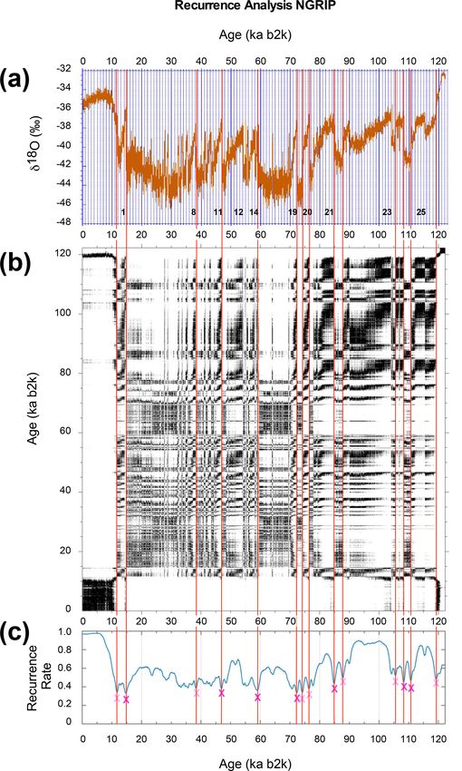
250                           D.-D. Rousseau et al.: Abrupt climate changes and the astronomical theory: are they related?

Although it is presently well acknowledged in the climate           the results of these estimates, he found that the summer in-
community, this mechanism underwent a long journey to               solation at 65◦ N is best correlated with glacial–interglacial
reach such general acceptance (Imbrie and Imbrie, 1979).            transitions, as determined by the study by Penck and Brück-
   In the 1840s, while visiting Scotland, Agassiz (1842) at-        ner (1909) of Alpine glaciations.
tributed erratic boulders noticed in the local landscape to for-       Milankovitch’s astronomical theory of climate was
mer ice age glaciers in the area, recalling his former obser-       severely criticized by contemporary physicists and rejected
vations in Switzerland (Agassiz, 1838). Meanwhile, Adhé-            by most Quaternary geologists, as isotopic C14 dating threw
mar (1842) proposed that glaciations, like those inferred by        the Günz–Mindel–Riss–Würm classification out the window
Agassiz from field observations, occurred every 22 000 years        (e.g., Flint, 1971, and references therein). Interest in this the-
due to the Earth’s evolving on an elliptic orbit with its ro-       ory was restored, however, as the pace of Quaternary cli-
tation axis tilted with respect to the orbital plane. Adhémar       mate changes – defined now by δ 18 O records from benthic
also concluded that, as the Southern Hemisphere receives            foraminifera (Emiliani, 1955) – was connected on a much
less solar radiation per year than the Northern Hemisphere          sounder basis with orbital variations in the seminal paper of
(Adhemar was relying on the number of the nights at the bo-         Hays et al. (1976). At the same time, Berger (1977, 1978), us-
real pole versus the number of nights at the austral pole), this    ing the much more accurate orbital calculations of Chapront
contributed to keeping temperatures cold enough to allow ice        et al. (1975), more reliably linked the insolation variations to
sheets to build up.                                                 the waxing and waning of the huge Northern Hemisphere ice
   It was 5 decades later that Croll (1890) presented his the-      sheets over North America, Greenland, Iceland, and Europe,
ory of the ice ages being driven by the changing distance           including the British Isles and Fennoscandia. The Quaternary
between the Earth and the Sun as measured on 21 Decem-              period, however, also shows an intriguing transition between
ber, which is due to the eccentricity of the Earth’s orbit and      the 40 kyr cycles that is dominant during the Early (or Lower)
the precession of the equinoxes. He used formulae for orbital       Pleistocene, i.e., from 2.6 up to 1.25 Ma, and the dominant
variations developed by Le Verrier (1858) and also stated           100 kyr cycles of the Middle Pleistocene and Late (or Up-
that, above a particular threshold, Northern Hemisphere win-        per) Pleistocene, i.e., the last 800 kyr, which show longer
ters would trigger an ice age, while below another thresh-          glacials that imply much larger continental ice sheets. The
old an ice age would develop in the Southern Hemisphere.            transition interval between 1.25 and 0.8 Ma, named the mid-
According to Croll’s theory, it is the slowly evolving eccen-       Pleistocene transition (MPT; Pisias and Moore, 1981; Ruddi-
tricity of the Earth’s orbit that is the key driver, with glacia-   man et al., 1989), experienced variability that does not appear
tions occurring only when eccentricity is high. He concluded,       to be directly linked to insolation changes at high latitudes. In
therefore, that eccentricity can impact the annual amount of        fact, the processes involved are not fully understood and are
heat received from the sun and also leads to differences in         still a matter of debate (Ghil and Childress, 1987, Sect. 12.7;
seasonal temperatures.                                              Ghil, 1994; Saltzman, 2002; Clark et al., 2021).
   Parallel to these physical calculations, observations of            Although the broad astronomic framework for past climate
frontal moraines in the Alpine valleys led to the identifi-         changes seems to be widely accepted, high-resolution inves-
cation of numerous glacial events in the past. Considering          tigations over the past decades in ice, marine, and terrestrial
the geometry and position of the terrace systems resulting          records revealed much shorter periodicities than the orbital
from these moraines in Alpine valleys, Penck and Brück-             ones, as well as abrupt changes that do not match the transi-
ner (1909) identified four main glaciations, determined from        tions attributed to variations in eccentricity, obliquity, or pre-
ice advances in the Alpine foreland: Günz, Mindel, Riss, and        cession of the equinoxes. This millennial variability, identi-
Würm. This sequence became the paleoclimate framework               fied initially during the last climate cycle (Dansgaard et al.,
for many decades, until the development of marine and ice           1982), has been described in older records, indicating that
coring programs.                                                    it prevailed during at least the past 0.5 Ma, as recorded in
   A total of 30 years after Croll, Milankovitch (1920, 1941),      marine records (McManus et al., 1999). The increased res-
inspired by his exchanges with Wladimir Peter Köppen and            olution of these records has shown that millennial climate
Alfred Wegener, provided a crucial step in advancing the            variability can be observed in all types of records, includ-
theory that major past climate changes had an astronomi-            ing in ice (Johnsen et al., 2001; Buizert et al., 2015a), ma-
cal origin resulting from the interaction between the eccen-        rine (Broecker, 2000; Shackleton et al., 2000), and terres-
tricity of the Earth’s orbit around the sun, the precession of      trial (Sanchez-Goni et al., 2000, 2002; Cheng et al., 2016)
the equinoxes, and the tilt of the Earth’s rotation axis. This      records associated with abrupt warmings or with strong (and
theory, often given his name today, implies a fairly regular,       massive) iceberg discharges into the North Atlantic Ocean
multi-thousand-year variability. Based on this crucial idea         (Ruddiman, 1977; Bond et al., 1992, 1993; Andrews and
and on using the recent orbital calculations of Pilgrim (1904),     Voelker, 2018) that correspond to particular cooling events.
among others, Milankovitch was able to estimate tempera-            Both hemispheres have been impacted by this millennial
tures and insolation at various latitudes at the top of the at-     variability through a mechanism described as the bipolar see-
mosphere and follow their variations through time. Among            saw (Stocker and Johnsen, 2003).

Clim. Past, 18, 249–271, 2022                                                            https://doi.org/10.5194/cp-18-249-2022
D.-D. Rousseau et al.: Abrupt climate changes and the astronomical theory: are they related? 251
In this paper, we show that abrupt climate changes are still to track the numerous glacial–interglacial cycles of the past
affected, albeit indirectly, by changes in insolation and hence 2.75 Myr with the help of variations in Earth’s orbital param-
in overall ice sheet volume. In this sense, the Milankovitch eters (Fig. S1). Besides these relatively slow variations, ev-
framework is shown herein to be quite relevant to the study of idence of millennial-scale variability can be observed since
abrupt and large climate changes. The paper is organized as the appearance of IRD in the North Atlantic at about 1.5 Ma.
follows. In Sect. 2, we describe the records and the methods This much faster variability is superposed upon the classical
used to identify the major transitions. In Sect. 3, major transi- orbital periodicities; see Fig. 3.
tions for the last 3.2 Myr of Northern Hemisphere climate are Observations of such abrupt variations have been reported
described. In Sect. 4, we concentrate on the millennial-scale in some detail for the last glacial period by the North Green-
variability revealed by these records. In Sect. 5, we establish land Ice Core Project at 75.1◦ N, 42.32◦ W (Barbante et al.,
a connection between Dansgaard–Oeschger (DO) events and 2006). The δ 18 O record best describes the more or less regu-
amended Bond cycles, and outline how global ice sheet vol- lar recurrence of cold and warm events that we are analyzing;
ume affects the latter. Concluding remarks follow in Sect. 6. see Fig. 1c.
2 Material and methods 2.2 The methods
2.1 The records
The increase in resolution of the Greenland ice cores (Fis-
cher et al., 2015; Schupbach et al., 2018; Svensson et al.,
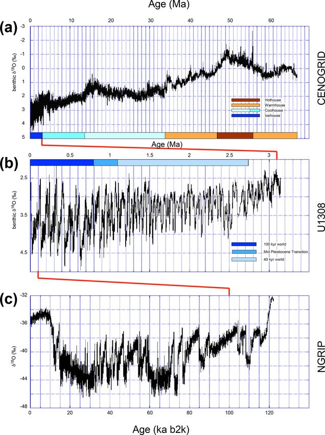
Over the past 66 Myr, corresponding to the Cenozoic Era, 2020) and of several speleothems (Cheng et al., 2016) al-
Earth’s climate has experienced four main states, from lowed much more detailed analyses not only of the δ 18 O
“Warmhouse” and “Hothouse” between 66 and 34 Ma to but also of other proxies, such as dust content, leading to
“Coolhouse” and “Icehouse” from 34 Ma until the present the identification of sub-events, as compiled by Rasmussen
time; see Fig. 1a. Although the first two states alternated et al. (2014). It is these high-resolution analyses that led to
in a warm–hot–warm sequence, the last two succeeded each defining the Greenland interstadials (GIs), followed by the
other, thus generating the classical climate trend towards the associated Greenland stadials (GSs). To gain further insight
recent ice age conditions (Zachos et al., 2001; Westerhold et into the climate story the records tell us, we performed a
al., 2020; Scotese et al., 2021). The last 3.3 Myr have been quantitative, objective analysis of these time series of proxy
defined as an Icehouse climate state, with the appearance variables based on two methods: the Kolmogorov–Smirnov
of the Northern Hemisphere ice sheets and their variations (KS) augmented test of Bagniewski et al. (2021) and the re-
through time (Westerhold et al., 2020). This Icehouse state is currence plots (RPs) of Marwan et al. (2007, 2013).
characterized by a change of the interplay between benthic Bagniewski et al. (2021) proposed a method based on an
δ 13 C and δ 18 O, which corresponds to a new relationship be- augmented nonparametric Kolmogorov–Smirnov (KS) test
tween the carbon cycle and climate. Indeed, the negative ex- to efficiently and robustly detect abrupt transitions in paleo-
cursions in δ 13 C were associated with negative ones in δ 18 O records. The classical KS test consists of quantifying and
during most of the Cenozoic since 66 Ma. A shift occurred, comparing the empirical distribution functions of two sam-
however, in the Plio-Pleistocene at about 5 Ma, with negative ples from a time series both before and after a potential jump.
δ 13 C excursions being associated with positive δ 18 O excur- In the present case, the test is augmented by varying window
sions (Turner, 2014). Such a shift appears to be related to a sizes and by evaluating the rate of change and the trend in
dichotomy in the response of the marine and terrestrial car- maxima and minima of the time series. This method allows
bon reservoirs to orbital forcings. one to reliably establish the main transitions in a record, such
The past 3.2 Myr of Northern Hemisphere climate are par- as the marine isotope stages in the U 1308 benthic δ 18 O or the
ticularly well described in North Atlantic core U1308 at GS–GI boundaries in the North Greenland Ice Core Project
49.87◦ N, 24.24◦ W (Hodell and Channell, 2016a). This core (Barbante et al., 2006) δ 18 O.
is located in the ice-rafted debris (IRD) of continental detri- The recurrence plots (RPs) were introduced by Eckmann
tal material eroded by the ice sheets (Ruddiman, 1977), and et al. (1987) into the study of dynamical systems and popu-
it yields a more complete record than U1313 (Naafs et al., larized in the climate sciences by Marwan et al. (2007, 2013).
2013); see Fig. 1b. The variations in the benthic δ 18 O mostly The purpose of RPs is to identify recurring patterns in a time
indicate varying periodicities through time that correspond series in general and in a paleoclimate time series in particu-
to periodicities in the orbital parameters of Earth’s climate lar.
(Hodell and Channell, 2016a; see Fig. S1 in the Supplement), The RP for a time series xi : i = 1, . . . , N is constructed as
as confirmed by Lisiecki and Raymo (2005) from the stack a square matrix in a Cartesian plane with the abscissa and or-
oxygen isotope record that they produced using 57 marine dinate both corresponding to a time-like axis, with one copy
records from the world’s oceans. xi of the series on the abscissa and another copy xj on the
The behavior of the U1308 proxy records on the timescale ordinate. A dot is entered into a position (i, j ) of the matrix
of many tens and hundreds of thousands of years allows us when xj is sufficiently close to xi . For more details – such
https://doi.org/10.5194/cp-18-249-2022 Clim. Past, 18, 249–271, 2022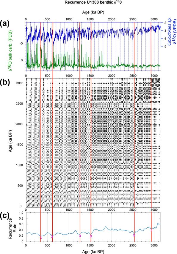
252                            D.-D. Rousseau et al.: Abrupt climate changes and the astronomical theory: are they related?

Figure 1. Earth climate history represented by two marine records and an ice core one. (a) Record of benthic δ 18 O of the CENOGRID stack
for the last 66 Myr; the hothouse, warmhouse, coolhouse, and icehouse intervals, following Westerhold et al. (2020), are indicated along
the abscissa. (b) Benthic δ 18 O record of the U1308 marine core (Hodell and Channell, 2016a) for the last 3.2 Myr; the 40 kyr, 100 kyr, and
mid-Pleistocene transition (MPT) intervals are indicated along the top of the diagram. (c) Record of 122 ka b2k δ 18 O of the NGRIP ice core
(Rasmussen et al., 2014) for the last 122 kyr b2k. Here “b2k” means before 2000 CE.

as how “sufficiently close” is determined – we refer to Eck-            xi than xi is to xj (Eckmann et al., 1987). An important ad-
mann et al. (1987) and to Marwan et al. (2013). Clearly, all            vantage of the RP method is that it does apply to dynamical
the points on the diagonal i = j have dots and the matrix is in         systems that are not autonomous, i.e., that may be subject to
general rather symmetric, although one does not always de-              time-dependent forcing. The latter is certainly the case for
fine closeness symmetrically; to wit, xj may be “closer to”

Clim. Past, 18, 249–271, 2022                                                                 https://doi.org/10.5194/cp-18-249-2022
D.-D. Rousseau et al.: Abrupt climate changes and the astronomical theory: are they related?                                   253

the climate system on timescales of 10–100 kyr and longer,          ternary, when the North American ice sheets were consider-
which are affected strongly by orbital forcing.                     ably larger.
   Eckmann et al. (1987) distinguished between large-scale             The second date corresponds to an increase in amplitude
“typology” and small-scale “texture” in the interpretation of       in ice volume variations between glacial maxima and inter-
square matrix of dots that is the visual result of RP. Thus,        glacial optima. This second step shows the permanent oc-
if all the characteristic times of an autonomous dynamical          currence of ice-rafted events during glacial intervals in the
system are short compared to the length of the time series,         record. The latter behavior signals a stronger relationship
the RP’s typology will be homogeneous and thus not very             between climate variations and Northern Hemisphere ice
interesting. In the presence of an imposed drift, a more inter-     sheets.
esting typology will appear. The most interesting typology in          The third date, close to the MIS22–24 δ 18 O optima, shows
RP applications so far is associated with recurrent patterns        increased continental ice volume in the Northern Hemisphere
that are not quite (but are close to being) periodic. Hence,        (Batchelor et al., 2019) but also more stability in the East
such patterns are not easily detectable by purely spectral ap-      Antarctic ice sheet in Southern Hemisphere (Jakob et al.,
proaches to time series analysis. Marwan et al. (2013) dis-         2020). In parallel, evidence of a major glacial pulse recorded
cuss how to render the purely visual RP typologies studied          in Italy’s Po Plain, as well as in 10 Be-dated boulders in
up to that point in a more objectively quantifiable way via         Switzerland, is interpreted as marking the onset of the first
recurrence quantification analysis and bootstrapping (Efron,        major glaciation in the Alps (Muttoni et al., 2003; Knudsen
1981; Efron and Tibshirani, 1986).                                  et al., 2020). At about the same time, the synthetic Green-
   The selection of the major transitions in the RPs was            land δ 18 O reconstruction of Barker et al. (2011), which starts
achieved by performing a recurrence rate (RR) analysis. The         at 800 ka, indicates the occurrence of millennial variability
values obtained for every record correspond to the mean for         expressed by DO-like events.
different window lengths ranging from 1 to 15 kyr. The selec-          The last date at 0.65 Ma marks the end of the transition
tion of the transitions of interest thus relies on the definition   from the Lower Pleistocene and Middle Pleistocene inter-
of a threshold that we choose to be the standard deviation          val – characterized by 41 kyr dominated cycles and smaller
of RR prominence, which is 0.089 for the U1308 benthic              23 kyr ones – to the Upper Pleistocene, with its 100 kyr
δ 18 O, 0.127 for the U1308 bulk carbonate δ 18 O, and 0.173        dominated cycles; see Fig. 1b. The sawtooth pattern of the
for NGRIP δ 18 O. The results were plotted along with the           interglacial–glacial cycles (Broecker and van Donk, 1970),
original recurrence plot (Table 1). Please see further details      which first becomes noticeable at 0.9 Ma, is well established
in Bagniewski et al. (2021).                                        during this final interval, in contradistinction with the pre-
                                                                    vious, more smoothly shaped pattern that appears to follow
                                                                    the obliquity variations. The global ice volume is maximal,
                                                                    exceeding the values observed earlier in the record, due in
3   The past 3.2 Myr history of the Northern                        large part to the larger contribution of the Northern Ameri-
    Hemisphere climate                                              can ice sheets. The latter now have a bigger impact on North-
                                                                    ern Hemisphere climate than the Eurasian ice sheets (Batch-
Analyzing the U1308 benthic δ 18 O record allows one to iden-       elor et al., 2019). The IRD event intensity and frequency of
tify the various transitions between the marine isotope stages      occurrence increased (McManus et al., 1999) as well, lead-
that covered the last 3.2 Ma and that were driven by varia-         ing to the major iceberg discharges into the North Atlantic
tions in the orbital parameters (Fig. S1). However, the RPs         named Heinrich events (HEs); see Heinrich (1988), Bond
reveal several key features that appear in the U1308 records        et al. (1992, 1993), and Obrochta et al. (2014). The inter-
during this time interval that are much more plausibly re-          val of 1–0.4 Ma is also the interval during which Northern
lated to processes other than the orbital forcing. Hoddell and      Hemisphere ice sheets reached a southernmost extent during
Channell (2016a) identified four major steps in their climate       MIS16 and MIS12, similar to the one reached during MIS6
record. These four steps are linked to thresholds in the ben-       (Batchelor et al., 2019).
thic and bulk carbonate δ 18 O variations, and they occur at           The benthic δ 18 O record of the U1308 marine-sediment
2.75, 1.5, 0.9, and 0.65 Ma.                                        core is interpreted in terms of global ice volume and deep-
   The first date is interpreted as corresponding to the earli-     ocean temperatures (Chappell and Shackleton, 1986; Shack-
est occurrence of IRD in the North Atlantic. This occurrence        leton, 2000; Elderfield et al., 2012). Its recurrence analysis
characterizes the presence of Northern Hemisphere coastal           shows a drift topology (Marwan et al., 2007, 2013) that char-
glaciers large enough to calve icebergs into the ocean, and         acterizes a monotonic trend in time, associated with nonsta-
the melting of these icebergs is likely to have impacted the        tionary systems with slowly varying parameters. Moreover,
oceanic circulation. Naafs et al. (2013) reported the occur-        the RP exhibits a characteristic texture given by the pat-
rence of minor IRD events, attributed mainly to Greenland           tern of vertical and horizontal lines that mark recurrences.
and Fennoscandian glaciers. These events indicate a greater         These lines sometimes form recurrence clusters that corre-
size of ice sheets over these regions than during the later Qua-    spond to specific periodic patterns. We thus identify five steps

https://doi.org/10.5194/cp-18-249-2022                                                            Clim. Past, 18, 249–271, 2022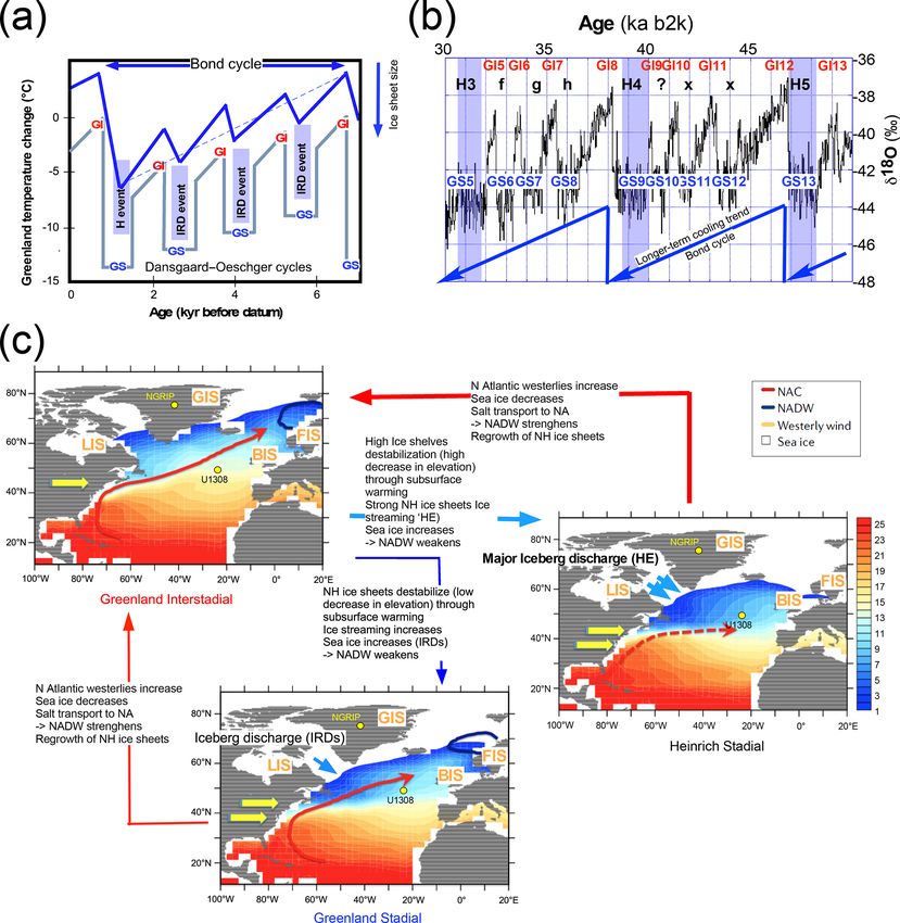
254 D.-D. Rousseau et al.: Abrupt climate changes and the astronomical theory: are they related?
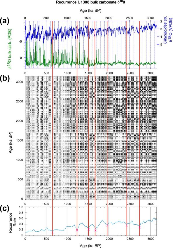
Table 1. Statistics of the recurrence rate analysis for U1308 benthic δ 18 O, U1308 bulk carbonate δ 18 O (Hodell and Channell, 2016a),
and NGRIP δ 18 O (Rasmussen et al., 2014). Dates where the recurrence rate (RR) prominence is higher than the RR standard deviation are
considered major transitions and are labeled with a red cross in Figs. 2c, 3c, and 4c. Periods with an RR prominence that is slightly lower than
the RR standard deviation are taken into account and labeled with a pink cross in the same figures. RR prominence significance is represented
in this table as follows: a shows prominence significance above the standard deviation (SD), and b shows prominence significance slightly
lower than the standard deviation.
U1308 δ 18 O U1308 bulk carbonate δ 18 O NGRIP δ 18 O
window: 60–250 ka window: 60–250 ka window: 1–15 ka
ka BP RR prominence Signif. ka BP RR prominence Signif. ka BP RR prominence Signif.
2524 0.238 a 2732 0.204 a 14.8 0.568 a
1510 0.142 a 1681 0.197 a 108.3 0.395 a
354 0.124 a 1510 0.135 a 72.3 0.361 a
614 0.112 a 1234 0.128 a 84.9 0.323 a
1248 0.087 a 1966 0.125 b 58.9 0.257 a
2925 0.071 b 653 0.122 b 47 0.238 a
879 0.071 2421 0.118 b 110.7 0.207 a
2741 0.070 2095 0.088 87.8 0.169 b
1736 0.066 856 0.072 119.3 0.152 b
1428 0.061 303 0.071 74.2 0.131 b
2430 0.060 3026 0.070 38.3 0.129 b
1975 0.057 2865 0.064 76.4 0.125 b
2141 0.051 447 0.061 105.5 0.102 b
132 0.040 2304 0.044 11.7 0.099 b
3041 0.037 2605 0.032 115.5 0.096
2054 0.037 1112 0.028 55.4 0.093
2984 0.030 2802 0.023 43.5 0.089
1073 0.024 28.4 0.086
64.3 0.082
23.6 0.080
35.6 0.079
77.8 0.068
104.2 0.059
33.3 0.047
51.6 0.046
70.7 0.045
89.9 0.045
95.3 0.042
48.6 0.039
41.5 0.028
54.5 0.022
in the δ 18 O variability; see Fig. 2a and c and Tables 1 and North Atlantic Ocean, with the most negative δ 18 O values
2. Two are roughly similar to those determined by Hoddell representing the largest iceberg calvings (Hodell and Chan-
and Channell (2016a), i.e., at 1.5 and 0.65 Ma, and three dif- nell, 2016a). The recurrence analysis of this record also dis-
fer, i.e., at 2.55, 1.25, and 0.35 Ma. Interestingly, the inter- plays the evolutionary trend represented by a drift topology,
val 1.25 to 0.65 Ma corresponds roughly to the previously and it yields one of the two Hodell and Channell (2016a)
mentioned MPT, during which a shift from climate cycles steps at 1.5 Ma, while the transition at 0.65 Ma is slightly
dominated by a 40 kyr periodicity to 100 kyr dominated ones below our threshold (Fig. 3a, c, Tables 1 and 2). Our anal-
occurred (Shackleton and Opdyke, 1977; Pisias and Moore, ysis further identifies the steps at 1.25, 1.65 and 2.75 Ma,
1981; Ruddiman et al., 1989; Clark and Pollard, 1998; Clark with the 1.25 step also noticed in the δ 18 O. Two other transi-
et al., 2006). A sixth transition at 2.95 Ma is close to the se- tions show a recurrence prominence close to our threshold at
lected threshold, as described at the end of Sect. 2.2. 1.95 and 2.45 Ma. Table 2, comparing the Hodell and Chan-
The δ 18 O bulk carbonate record in the U1308 core is nell (2016a) steps with the thresholds detected by the RP,
in turn interpreted as characterizing IRD released into the
Clim. Past, 18, 249–271, 2022 https://doi.org/10.5194/cp-18-249-2022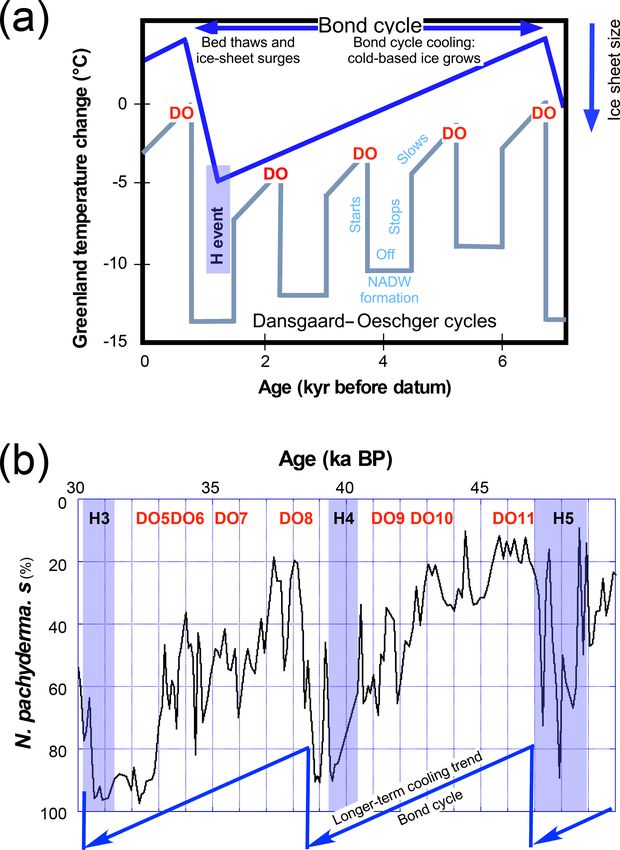
D.-D. Rousseau et al.: Abrupt climate changes and the astronomical theory: are they related?                                            255

Table 2. Comparison of the main steps detected by Hodell and Channell (2016a) from the U1308 marine record with those deduced from
the recurrence plot of the benthic δ 18 O and bulk carbonate δ 18 O data of the same record. RR prominence significance is defined the same
way as in Table 1.

    Hodell and Channell    Benthic δ 18 O   Benthic δ 18 O   Signif. benthic      Bulk carbonate      Bulk carbonate     Signif. bulk
    (2016a) main steps       thresholds       thresholds     δ 18 O thresholds   δ 18 O thresholds   δ 18 O thresholds   carbonate δ 18 O
    in Ma                         in Ma                RR    RR                              in Ma                 RR    thresholds RR
                                     2.93          0.0707    a
    2.75                                                                                     2.73             0.2036     a
                                     2.52          0.2380    a                               2.42             0.1176
                                                                                             1.97             0.1250     b
                                                                                             1.68             0.1975     a
    1.5                              1.51          0.1417    a                               1.51             0.1349     a
                                     1.25          0.0869    b                               1.23             0.1275     a
    0.9
    0.65                             0.61          0.1115    a                               0.65             0.1222     b
                                     0.35          0.1240    a

                           SD = 0.0890                                           SD = 0.1272

shows that the former are mainly related to the IRD history             briefly in the previous section, and it allowed us to track
of the past 3.3 Ma.                                                     the numerous glacial–interglacial cycles of the past 2.75 Myr
   The 1.25 Ma date is particularly significant, since it is fol-       with the help of variations in Earth’s orbital parameters; see
lowed by an increase in the amplitude of glacial–interglacial           Fig. S1 in the Supplement. Besides these relatively slow vari-
fluctuations (Fig. 2a). The interval 2.8 to 1.2 Ma shows                ations, evidence of millennial-scale variability can be ob-
glacial–interglacial sea level variations of about 25–70 m              served since the appearance of IRD in the North Atlantic at
below the present-day value (van de Wal et al., 2011).                  about 1.5 Ma; this much faster variability is superposed upon
The reconstructed CO2 concentrations varied between 270                 the classical orbital periodicities (Fig. 3).
and 280 ppmv during interglacials and between 210 and                      Detailed observations of such abrupt variations have been
240 ppmv during glacials, with a decreasing trend of about              reported for the last glacial period, with the more or less reg-
23 ppmv over this 1.4 Myr long interval (van de Wal et                  ular recurrence of cold and warm events; see Fig. 1c. The for-
al., 2011). After 1.25 Ma, the sea level changes increased              mer are represented by IRD events, some of which are signif-
to about 70–120 m below the present-day value, while                    icantly stronger and represent the previously mentioned HEs
the reconstructed CO2 concentrations varied between 250                 that correspond to massive discharges of icebergs into the
and 320 ppmv during interglacials and between 170 and                   North Atlantic (Heinrich, 1988; Bond et al., 1992; McManus
210 ppmv during glacials (Berends et al., 2021). Similar vari-          et al., 1994; Hemming, 2004).
ations were determined by Seki et al. (2010), although pCO2                Abrupt warmings happening over as little as a few decades
changes that occurred before the time reached by ice core               each have been inferred from Greenland ice cores (Dans-
records are associated with high uncertainties in both dating           gaard et al., 1993; Clark et al., 1999) and labeled DOs or
and values. The “Milankovitch glacials”, which correspond               Greenland interstadials (GIs: Rasmussen et al., 2014); see
to the odd marine isotope stages determined in the U1308                Fig. 4a. These warm events are followed by a return to
core and in many others, have maxima that are characterized             glacial conditions, called Greenland stadials (GSs). This re-
by low eccentricity and obliquity, and a boreal summer that             turn generally happens in two steps, thus forming DO cycles
coincides with aphelion and leads and, therefore, to mini-              of variable duration that do not exceed a millennial timescale
mum values of summer insolation. The increase in IRD vari-              (Broecker, 1994; Boers et al., 2018; Boers, 2018, and refer-
ability and magnitude since 1.5 Ma (Hodell and Channell,                ences therein). Broecker (1994) does not provide any precise
2016a), however, shows that distinct, faster processes have             DO timescale but indicates that “climate cycles [average] a
to be considered due to slow changes in Earth’s orbital pa-             few thousands of years in duration”. Boers et al. (2018) do
rameters; see again Figs. 2 and 3.                                      not yield any exact value for the DO timescales either, but
                                                                        Fig. S1 in their appendix does indicate the durations of the
                                                                        stadials and interstadials in the NGRIP record varying be-
4   Millennial-scale variability                                        tween 340 and 8365 years and between 190 and 16 440 years
                                                                        respectively.
The behavior of the U1308 proxy records on the timescale of
many tens and hundreds of thousands of years was described

https://doi.org/10.5194/cp-18-249-2022                                                                  Clim. Past, 18, 249–271, 2022
256 D.-D. Rousseau et al.: Abrupt climate changes and the astronomical theory: are they related? Figure 2. Recurrence analysis of the δ 18 O record in U1308 Cibicidoides sp. (Hodell and Channell, 2016a). (a) Time series of the Cibicidoides sp. δ 18 O (blue curve, top) and of the bulk carbonate δ 18 O (magenta curve, bottom). (b) Recurrence plot (RP) where the proximity threshold is 1(δ 18 O) = 0.2 ‰. (c) Recurrence rate (RR) with significant values labeled with a red cross; RR close to the threshold is marked in pink. Vertical bars represent the major transitions (5 + 1) determined by the analysis. The RP website is http://www.recurrence-plot.tk/ (last access: 8 February 2022). Numerous DO timescales have been published by Ras- as estimated by Rasmussen et al. (2014). It shows that the av- mussen et al. (2014), Wolff et al. (2010), Rousseau et erage duration of a DO cycle is of 4045 ± 3179 years. As the al. (2017a, b), and most recently Capron et al. (2021). How- periodicity of the events is at millennial and sub-millennial ever, no DO cycle timescale has been published as of yet. scale (Broecker, 1994; Clark et al., 1999; Ganopolski and Table 3 reports the duration of the DO cycles as expressed Rahmstorf, 2001; Rahmstorf, 2002; Schulz, 2002; Menviel by the interval between the start of a GI and the end of a GS et al., 2014; Lohmann and Ditlevsen, 2018, 2019) it corre- Clim. Past, 18, 249–271, 2022 https://doi.org/10.5194/cp-18-249-2022
D.-D. Rousseau et al.: Abrupt climate changes and the astronomical theory: are they related?                                             257

Figure 3. Recurrence analysis of U1308 bulk carbonate δ 18 O (Hodell and Channell, 2016a). Panel (a) is the same as Fig. 2a.(b) RP of the
bulk carbonate δ 18 O, with the same proximity threshold as in Fig. 2a. Panel (c) is the same as in Fig. 2c, except that the vertical bars now
represent the major thresholds (4 + 3) determined by the RR analysis in panel (c). The RP website is http://www.recurrence-plot.tk/.

sponds to processes that cannot be related to any orbital forc-          Zagwijn, 1989). The existence and dating of the DOs was
ing (Lohmann et al., 2020) but rather to factors that are in-            initially questioned as they had not been observed in marine
trinsic to the Earth system.                                             cores in the 1970s and 1980s (Broecker et al., 1988; Broecker
   DO events were first observed in the various ice cores                and Denton, 1989). However, Dansgaard et al. (1993) clearly
retrieved from the Greenland ice sheet (Dansgaard et al.,                identified 23 rapid warming events during the last climate
1969; Johnsen et al., 1972). Some of these DOs were cor-                 cycle from the Greenland GRIP ice core.
related to European warm interstadials, which had been de-                  These 23 DO events were later confirmed in other Green-
scribed from pollen records (Woillard, 1978; Behre, 1989;                land ice cores (Johnsen et al., 2001), following the initial

https://doi.org/10.5194/cp-18-249-2022                                                                    Clim. Past, 18, 249–271, 2022
258                             D.-D. Rousseau et al.: Abrupt climate changes and the astronomical theory: are they related?

Figure 4. Recurrence analysis of NGRIP δ 18 O. (a) NGRIP δ 18 O variations over the last 122 kyr b2k (Rasmussen et al., 2014); selected
canonical Dansgaard-Oeschger (DO) events are indicated on the abscissa by the numbers assigned by Dansgaard et al. (1993). (b) RP of the
time series in panel (a) above; the proximity threshold here is 1(δ 18 O) = 1.3 ‰. (c) Recurrence rate analysis showing the selected thresholds
(7 + 7) indicated by the vertical bars. The RP web site is http://www.recurrence-plot.tk/.

correlation of rapid changes between Camp Century and                     Fig. 4a. Moreover, the 23 canonical DOs were described later
Dye3 ice cores (Dansgaard et al., 1982), and they are con-                using various types of records in marine sediments (Bond
sidered the “canonical” DOs. They were assigned numbers                   et al., 1992; Henry et al., 2016) and in terrestrial sediments
that increase sequentially downcore, with no. 1 allocated to              (Allen et al., 1999; Sanchez-Goni et al., 2000, 2002; Müller
the Bølling pollen oscillation (Dansgaard et al., 1993); see              et al., 2003; Fletcher et al., 2010; Rousseau et al., 2017a,

Clim. Past, 18, 249–271, 2022                                                                   https://doi.org/10.5194/cp-18-249-2022
D.-D. Rousseau et al.: Abrupt climate changes and the astronomical theory: are they related?                                          259

Table 3. Thresholds identified in the recurrence plot of NGRIP δ 18 O record and their correspondence in the marine isotope stratigraphy of
the last climate cycle stratigraphy (Bassinot et al., 1994; Lisiecki and Raymo, 2005). RR prominence significance as in Table 1.

                              NGRIP δ 18 O     NGRIP δ 18 O    Signif.    Marine isotope    LR04     Bassinot
                              thresholds in      thresholds               stratigraphy        age         age
                              ka (b2k)                  RR                boundaries         (ka)        (ka)
                              14.8                   0.5683    a          1/2                  14          11
                              38.3                   0.1293               2/3                  29          24
                              47.0                   0.2379    a          3/4                  57          57
                              58.9                   0.2571    a          4/5                  71          71
                              72.3                   0.3610    a          5.1 (peak)           82          79
                              74.2                   0.1308               5/5a               84.5        82.5
                              76.4                   0.1249               5.2 (peak)           87          86
                              84.9                   0.3229    a          5a/5b              91.5        91.5
                              87.8                   0.1689    b          5.3 (peak)           96          97
                              105.5                  0.1020               5b/5c             102.5       101.5
                              108.3                  0.3953    a          5.4 (peak)          109         106
                              110.7                  0.2068    a          5c/5d               116         114
                              119.3                  0.1520    b          5.5 (peak)          123         122
                                                                          5/6                 130         127
                              SD = 0.1732

b, 2021), including speleothems (Wang et al., 2001; Genty                Henry et al., 2016), with the Greenland climate leading
et al., 2003; Fleitmann et al., 2009; Boch et al., 2011). The            Antarctica by approximately 200 years. On the other hand,
transitions identified by a KS test in the NGRIP δ 18 O include          Knorr and Lohmann (2003) suggest a true south to north di-
all the canonical events described by Dansgaard et al. (1993)            rection of climate change propagation. At this point, one can
and identified in Rasmussen et al. (2014), although a few                only state that the latter observational studies do not contra-
other DOs or sub-events are not detected by it even after                dict the earlier modeling studies but also do not directly con-
changing the test window size; see Fig. S2.                              firm them either.
   Using a global climate indicator like methane (CH4 ) Blu-                Many DO models – e.g., Buizert and Schmittner (2015),
nier and Brook (2001), EPICA Community Members (Bar-                     Dokken et al. (2013), Ganopolski and Rahmstorf (2001),
bante et al., 2006) and the WAIS Consortium (Buizert et al.,             Lohman and Ditlevsen (2018, 2019), Peltier and Vet-
2015a, b) demonstrated that the millennial-scale variations              toretti (2014), Shaffer et al. (2004), Klockmann et al. (2018),
observed during the last 130 kyr in Greenland are observed               Menviel et al. (2014, 2021), and Timmermann et al. (2003) –
in Antarctica as well and that they are thus a global phe-               have not specifically addressed the issue of the interhemi-
nomenon. Hinnov et al. (2002) also carried out an investi-               spheric signal’s direction. To address this issue, Boers et
gation on the methane-linked GISP2 and Byrd ice cores, in-               al. (2018) recently developed a simple model to reconstruct
cluding a statistically constrained spectral coherency anal-             the millennial variability in δ 18 O of the past 60 kyr b2k,
ysis demonstrating the global reach of the DO cycles. The                as observed in the high-resolution ice cores from NGRIP
δ 18 O variations in the two hemispheres are in opposite phases          in Greenland and the West Antarctic ice sheet (WAIS) in
though, with the Southern Hemisphere warmings occurring                  Antarctica. This simple model, based on the bipolar seesaw
prior to the Northern Hemisphere ones.                                   mechanism (Stocker and Johnsen, 2003), combines the inter-
   Several hypotheses have been proposed to determine                    actions between ice shelves and sea ice extents, subsurface
whether the climatic signal propagated between the two                   water temperatures in the North Atlantic Ocean, atmospheric
hemispheres is in a southward or northward direction. Vari-              temperature in Greenland, AMOC strength, and δ 18 O in both
ations in the Atlantic meridional overturning circulation                Greenland and Antarctica. The interplay of the feedbacks in-
(AMOC) play a key role in this teleconnection, as AMOC                   volved allowed the authors to reproduce the millennial-scale
slowdown during GSs corresponds to reduced oceanic north-                variability observed in both hemispheres despite the lack of
ward heat transport (Sarnthein et al., 2001; Ganopolski and              any time-dependent forcing that would involve orbital pa-
Rahmstorf, 2001; McManus et al., 2004). This reduction                   rameters.
does not contradict the southward propagation direction of
the climate signal, as documented by detailed high-resolution
marine-sediment and ice core studies (Buizert et al., 2015b;

https://doi.org/10.5194/cp-18-249-2022                                                                   Clim. Past, 18, 249–271, 2022
260 D.-D. Rousseau et al.: Abrupt climate changes and the astronomical theory: are they related?
5 DO events and bond cycles DO event (Bond et al., 1992; Alley, 1998; Alley et al., 1999;
Clark et al., 2007). This cooling trend ends with a final and
The results outlined in the previous section have led us to coldest GS that coincides with an HE. These groupings have
concentrate on the canonical DOs for which the tempera- been named Bond cycles (Broecker, 1994; Alley, 1998), and
ture reconstruction has been proposed based on 15 N mea- they have mainly been observed in North Atlantic marine
surements from the Greenland ice (Guillevic et al., 2014). records of the last climate cycle with a rough periodicity of
These estimates indicate that the 21 warming events during 7 kyr (Clark et al., 2007); see Fig. 6a, b. These Bond cycles,
the last climate cycle, between 12 and 87 ka b2k, had a range like the DO cycles, have no relationship with the periodicity
of 10–12 ◦ C on average (Kindler et al., 2014), with each tran- of the orbital parameters (Table S1), but they are in excellent
sition lasting between 50 and 100 years on average (Wolff et agreement with the robust 6–7 kyr periodicity of a natural, in-
al., 2010; Rousseau et al., 2017a, b, 2021), as found at least trinsic paleoclimate oscillator (Källèn et al., 1979; Ghil and
near the top of the Greenland ice sheet at the coring site. Not Le Treut, 1981).
only does the change in temperature over such a short time This oscillator is based on the countervailing effects of the
imply a drastic reorganization of the atmospheric and associ- positive ice–albedo feedback on Earth’s radiation balance –
ated marine circulations (Boers et al., 2018), but the timing with temperatures drops that are enhanced by the increas-
does not correspond to any periodicity of the orbital param- ing extent of sea ice (Budyko, 1969; Sellers, 1969) – and of
eters, either in the average duration of the events or in the the negative precipitation–temperature feedback on the mass
average interval between two such events; see Fig. S2. balance of ice sheets, with temperature increases that con-
The recurrence analysis performed on the high-resolution tribute to increased accumulation of the ice (Källèn et al.,
NGRIP δ 18 O record and illustrated in Figs. 4b and 5b sug- 1979; Miller and De Vernal, 1992; Ghil, 1994; Tziperman
gests looking for other mechanisms that might cause the and Gildor, 2003). Ghil and Tavantzis (1983) showed that the
abrupt changes mentioned previously. As for the δ 18 O record oscillator’s 6–7 kyr periodicity is quite stable over a substan-
analysis in core U1308 displayed in Figs. 2 and 3, the NGRIP tial range of parameter values, and Ghil (1994) noted that
study shows a drift topology with a non-uniform pattern. The this periodicity was predicted by Källén et al. (1979), well
RP shows changes in the system’s regime of behavior, as before the HEs were discovered by Heinrich (1988). More
identified by transitions detected by analyzing the RR values. recently, the HEs’ approximate recurrence time was found
The RR analysis of the NGRIP δ 18 O values identified seven to be roughly equal to this periodicity by Clark et al. (2007,
major transitions. Seven more indicate an RR close to the se- and references therein), in spite of the fact that these authors
lected threshold; see Tables 1 and 3. Numerous thresholds were not aware of its theoretical prediction by Michael Ghil
identified correspond to key dates of the last climate cycle and colleagues (Källèn et al., 1979; Ghil and Le Treut, 1981;
stratigraphy (Bassinot et al., 1994; McManus et al., 1994; Ghil, 1994).
Kukla et al., 1997; Lisiecki and Raymo, 2005; Clark et al., The HEs are believed to first occur at about 0.65 Ma, as
2009); see Table 3. can be deduced from the U1308 bulk carbonate δ 18 O records.
When plotted in Fig. 5c against the variations in global The GSs’ duration has sometimes been incorrectly linked
sea level deduced from North Atlantic and equatorial Pacific with the occurrence of an HE, leading to the misinterpreta-
δ 18 O benthic records by Waelbroeck et al. (2002), the length tion of HEs as being equivalent to GSs. A detailed study of a
of the GIs appears to be related to the mean sea level; see subset of GSs has demonstrated that HEs did not last the en-
Fig. S3. The long GIs occurred between 120 and 80 ka b2k tire duration of a GS (Guillevic et al., 2014), indicating much
and between 59 and 40 ka b2k. During these two intervals, more complex dynamics in the cold stadials themselves than
the global sea level exhibited relatively slight variations be- had initially been considered. Such complex climate behav-
tween about −15 and −45 m and about −50 and −75 m, ior, by extension, may have prevailed since the first occur-
respectively. Conversely, after 80 and after 32 ka b2k, GIs rence of HEs in the North Atlantic at about 0.65 Ma. More-
were shorter and occurred during the most abrupt drops in over, Bond and Lotti (1995) demonstrated that although an
sea level of the last climate cycle, from −15 to −85 m and HE was embedded into the final GS of the Bond cycles, ad-
from −75 m down to a minimum of about −120 m during the ditional IRD events of lower magnitude than an HE were also
Last Glacial Maximum. The agreement between the results embedded in the previous and intermediary GSs.
of the recurrence analysis and the NGRIP δ 18 O transitions, Therefore, the previous definition of the Bond cycles given
as well as the link between the length of GIs and the global by Lehman (1993), Broecker (1994), and Alley (1998) could
sea level variations, seems to establish a relation between the be revisited by including the IRD events embedded in ev-
variation in GI length and the spatial extent and elevation of ery stadial (Fig. 7a, b). Thus, Bond cycles should be inter-
the largest continental ice sheets, especially in the Northern preted as a sequence of DO cycles that starts with a distinctly
Hemisphere, with the latter expanding further inland and out warm GI that is followed by a cooling trend with increasingly
onto the continental shelf during the last climate cycle. colder GSs that include as many IRD events as the stadials
The DO cycles have been grouped together following an being identified, the latest of which is an HE; see Fig. 6a, b.
overall cooling trend of the GSs and subsequent to a strong
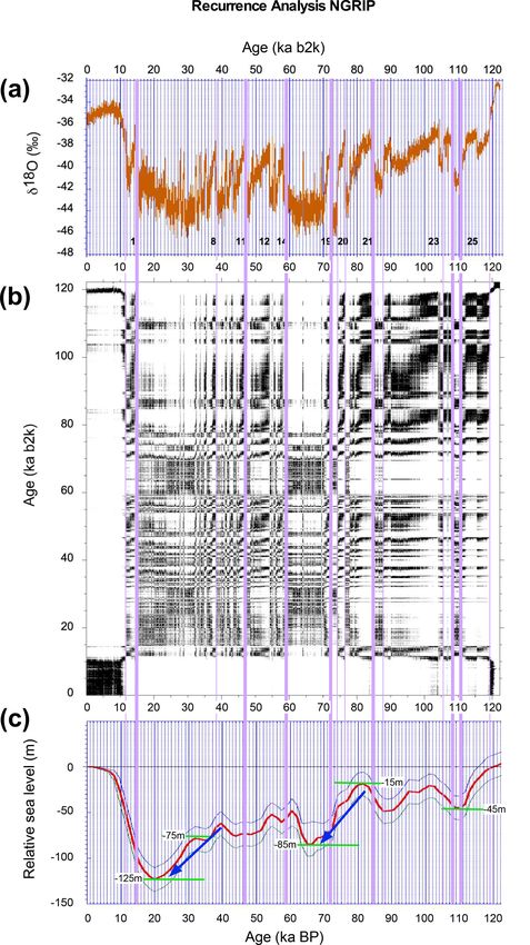
Clim. Past, 18, 249–271, 2022 https://doi.org/10.5194/cp-18-249-2022D.-D. Rousseau et al.: Abrupt climate changes and the astronomical theory: are they related? 261 Figure 5. Recurrence analysis of NGRIP δ 18 O. (a) NGRIP δ 18 O variations over the last 122 kyr b2k (Rasmussen et al., 2014); same as in Fig. 4a. Panel (b) is the same as Fig. 4b. (c) Variation of the sea level over the last 122 kyr BP as reconstructed from benthic δ 18 O foraminifera by Waelbroeck et al. (2002). The bold red line is the global mean sea level (m) below present, and the light blue lines are the minimum and maximum global mean sea level values (m) below present. The horizontal green line segments indicate some key sea levels. The RP web site is http://www.recurrence-plot.tk/. https://doi.org/10.5194/cp-18-249-2022 Clim. Past, 18, 249–271, 2022
262                            D.-D. Rousseau et al.: Abrupt climate changes and the astronomical theory: are they related?

                                                                       ing the much older time interval 1235–1220 ka, i.e., MIS41–
                                                                       37, from a marine record on the Iberian Margin. Although de-
                                                                       tecting variations in planktonic δ 18 O that are comparable to
                                                                       the MIS3 DO events in intensity and sawtooth shape, Birner
                                                                       et al. (2016) indicate that
                                                                            identifying further Bond-like cycles in MIS38 and
                                                                            40 is ambiguous. Although the lack of additional
                                                                            cycles might be due to the short duration of glacials
                                                                            in the 41 ka world, the occurrence of Bond-like cy-
                                                                            cles in the Early Pleistocene would not necessarily
                                                                            be expected, owing to their intrinsic relationship to
                                                                            Heinrich events (Bond et al., 1993) that have not
                                                                            been observed in the Early Pleistocene (Hodell et
                                                                            al., 2008).
                                                                       Specifically, the closing stadial of these cycles does not show
                                                                       a massive IRD discharge or HE as described during the last
                                                                       climate cycle.
                                                                          However, since IRD delivery to the North Atlantic requires
                                                                       ice sheets to reach the ocean, and since the first IRDs are
                                                                       recorded in the North Atlantic at about 1.5 Ma (Hodell and
                                                                       Channell, 2016a), one could assume that the start of this type
                                                                       of millennial variability occurred as early as this older thresh-
                                                                       old. Whether a younger start date of 0.9 Ma or an older one of
                                                                       1.5 Ma is posited, these dates show that the Northern Hemi-
                                                                       sphere ice sheets played a significant role in the onset of mil-
                                                                       lennial and sub-millennial climate variability that prevailed
                                                                       during the Middle Pleistocene and Late Pleistocene.
                                                                          Ziemen et al. (2019) simulated HEs following the binge–
Figure 6. Description of a Bond cycle. (a) Idealized Bond cycle
                                                                       purge model of MacAyeal (1993) and reported a two-step
as illustrated following Alley (1998). DO stands for Dansgaard–
                                                                       mechanism. The first step is a surge phase with enhanced
Oeschger event, H event stands for Heinrich event, and NADW
stands for North Atlantic Deep Water. (b) Variations in the percent-   fresh water discharge weakening the deep water formation
age of Neogloboquadrina pachyderma (s.), a species indicative of       due to the stratification of the surface water, increased sea
cold surface water, from DSDP 609 (Bond et al., 1992), illustrat-      ice cover, and leading to reduced North Atlantic sea sur-
ing two Bond cycles. These cycles show a series of Dansgaard–          face temperature due to a weakened AMOC, reduced evap-
Oeschger (DO) cycles composed of an abrupt warming that is fol-        oration, and precipitation. The second step corresponds to a
lowed by a return to glacial conditions represented by “stadials”.     post-surge phase with a much-lowered elevation of the Lau-
Every Bond cycle corresponds to a long-term cooling trend that         rentide ice sheet that may have lost several hundreds of me-
starts with a strong warming and ends with a stadial that includes a   ters or more during the massive iceberg discharges. During
massive iceberg discharge into the North Atlantic; Heinrich events     the post-surge phase described by Ziemen et al. (2019), a
are marked by a letter “H” followed by a number assigned by Bond
                                                                       higher sea level associated with the lower elevation of the
et al. (1992).
                                                                       ice sheet favors the northern polar jet moving northwards,
                                                                       which leads to more precipitation over Hudson Bay, speeds
                                                                       up the regrowth of the Laurentide ice sheet, and results in
   The synthetic Greenland δ 18 O record reconstructed from            the start of a new Bond cycle. A similar mechanism, albeit
the EPICA data over the last 800 kyr by applying the bipo-             of lower magnitude, could be considered for the other ice-
lar seesaw model (Barker et al., 2011) indicates that DO               berg discharges occurring during the GS, which did not yield
cycles have occurred at least during this time interval. Fur-          HEs. Such a mechanism may apply, with reduced amplitude,
thermore, this synthetic record is well correlated with δ 18 O         to the smaller Eurasian ice sheets that were also involved in
variations observed from Chinese speleothems (Cheng et                 the release of icebergs during HEs. The Ziemen et al. (2019)
al., 2016). Hence, the millennial variability associated with          mechanism appears, moreover, to be in agreement with the
the DO cycles is likely to have existed since 0.8 Ma, or               Mg / Ca data on benthic foraminifera studied by Marcott et
even since 0.9 Ma, when the global ice volume strongly in-             al. (2011). These authors found that warming of the subsur-
creased, as indicated by MIS22 δ 18 O and sea level values.            face temperature of the high-latitude North Atlantic led to
Birner et al. (2016) report millennial variability already dur-        increased basal melting under ice shelves, accelerated their

Clim. Past, 18, 249–271, 2022                                                              https://doi.org/10.5194/cp-18-249-2022
D.-D. Rousseau et al.: Abrupt climate changes and the astronomical theory: are they related? 263 Figure 7. Schematic diagram of the proposed updated Bond cycle. (a) The amended scheme here differs from the one in Fig. 6a by adding the IRD event associated to every Greenland stadials (GS). The canonical DO are labeled here Greenland interstadials (GI). (b) The revised cycle here differs from the one in Fig. 6a by using the NGRIP δ 18 O data (Rasmussen et al., 2014) to mark the GSs and GIs. IRD events observed in contemporaneous marine records by Bond and Lotti (1995), are indicated by the letters “f” to “h”, while IRD events that were observed but not assigned a number also by Bond and Lotti (1995), are indicated by a letter “x”. HE numbers are the same as in Fig. 5. (c) Maps illustrating the climate evolution associated with the “long-term cooling trend” that corresponds to a Bond cycle in panel (a). The last DO cycle, named a Heinrich stadial, is characterized by a massive release of icebergs. Annual mean sea surface temperature (◦ C) for a GI (here 47 ka), a GS (here 44.4 ka), and a Heinrich stadial (at 48 ka), as simulated in a transient experiment of MIS3 (Menviel et al., 2014, 2021). GIS stands for Greenland ice sheet, LIS stands for Laurentide ice sheet, BIS stands for British Isles ice sheet, and FIS stands for Fennoscandian ice sheet. https://doi.org/10.5194/cp-18-249-2022 Clim. Past, 18, 249–271, 2022
264                          D.-D. Rousseau et al.: Abrupt climate changes and the astronomical theory: are they related?

collapse as suggested by Boers et al. (2018), and drove the        Saltzman (2002) and Crucifix (2012) – while Hodell and
Hudson Strait Ice Stream of the Laurentide ice sheet to re-        Channell (2016a) only considered it as noise superimposed
lease IRD deposited as HEs (Alvarez-Solas and Ramstein,            on the orbital variability deduced from their wavelet analy-
2011); see Fig. 7c.                                                sis of the benthic δ 18 O record of U1308. Substantial, nonlin-
   Guillevic et al. (2014) studied 17 O excess variations in       ear interactions between internal oscillatory variability and
Greenland ice cores, which characterize changes in the             orbital forcing are actively being explored by Riechers et
lower-latitude hydrological cycle, and reported that, at least     al. (2021) in this special issue.
for HE4 and HE5, iceberg delivery to the North Atlantic did
not last the whole GS duration. Instead, this delivery oc-         6    Concluding remarks
curred about a hundred years after the start of the GS. This
short interval seems to correspond to the time during which        Our quick overview of millennial-scale climate variability
the subsurface warming of the ocean was linked to an ex-           over the last 3.2 Myr suggests the following conclusions.
pansion of the sea ice and the ice shelves, as initially men-
tioned by Marcott et al. (2011) and Boers et al. (2018), and           – The key phenomena that characterize this millennial-
it also corresponds to “pre-surge” conditions. According to              scale variability are Heinrich events (HEs), Dansgaard–
the Ziemen et al. (2019) model, increasing the flow of ice be-           Oeschger (DO) events, and Bond cycles. Abrupt
yond a certain threshold leads to the massive calving of ice-            changes are intimately interwoven with these phenom-
bergs (surge phase). Furthermore, Guillevic et al. (2014) in-            ena.
dicate that the HE4 post-surge started during GS9, hundreds
                                                                       – Present investigations – including both recurrence plot
of years prior to the start of the warming corresponding to
                                                                         (RP) analysis and Kolmogorov–Smirnov (KS) method-
GI8.
                                                                         ology – point to internal mechanisms being responsi-
   These sequences – starting with a strong GI, followed by
                                                                         ble for these millennial-scale events and for the associ-
intermediary GSs that include IRD events, and ending with
                                                                         ated abrupt changes. These mechanisms include internal
a colder GS that includes an HE (see Fig. 7a,b) must have
                                                                         oscillations of the ice sheet–ocean–atmosphere system
repeated throughout the last climate cycle, most likely dur-
                                                                         and episodic calving of ice sheets.
ing the glacial interval from 116 ka b2k covered in Bond and
Lotti (1995). In fact, HEs are believed to have first occurred         – The Bond cycles are linked to the dynamics of the
at about 0.65 Ma, although DO events may have occurred in-               Northern Hemisphere ice sheets, specifically to varia-
dependently since about 0.8 or even 0.9 Ma. It thus appears              tions in their spatial extent and their elevation. The clas-
that the millennial and sub-millennial variability correspond-           sical Bond cycles end with massive iceberg discharges
ing to the Bond cycles involves variations in size and ele-              into the North Atlantic Ocean mainly from the Lauren-
vation of the Northern Hemisphere ice sheets that give rise              tide ice sheet but also from the Fennoscandian, Green-
to the iceberg release events into the North Atlantic; see               land, Iceland, and British ice sheets. IRD releases to the
Fig. 7c. This mechanism may have played a key role dur-                  North Atlantic have also been documented during every
ing the past 0.8–0.9 Myr, when the Northern Hemisphere ice               stadial. Therefore, a link with the Northern Hemisphere
sheets were at their maximum size and extended out over the              ice sheet extents appears evident in order to allow ice-
continental shelf. This combination of size and contact with             berg calving into the North Atlantic, whatever the mag-
the much warmer ocean is likely to have destabilized the ice             nitude of the calving event, i.e., either IRD events or
sheets around the North Atlantic and have led to massive IRD             HEs. These Bond cycles in their new interpretation il-
events. The appearance of IRD in the North Atlantic Ocean,               lustrate a much more complex millennial variability
however, might have occurred as early as 1.5 Ma (Hodell and              than initially contemplated by not considering the DO
Channell, 2016a), a fact that might suggest the prevalence of            and HE individually but instead linking them into a uni-
the variability over short periods discussed herein over the             fied story.
last 1.5 Myr.
   In any case, a time interval of the most recent 0.8 or              – Millennial-scale variability is observed in proxy records
1.5 Myr seems to have witnessed millennial-scale climate                 from the very beginning of the last glacial period and
variability with an amplitude that exceeded the one due to the           during previous glacial periods, at least since 0.8–
direct forcing by the orbital periodicities (Ghil and Childress,         0.9 Ma, when HEs first appear in the records. This tim-
1987; Ghil, 1994; Riechers et al., 2021). This fairly agreed-            ing seems to coincide roughly with the MPT that has
upon fact lends support to the interpretation of the enhanced            been associated with a global increase in ice volume on
millennial variability during glacial times as arising from an           Earth. This coincidence does not exclude the possibility
internal oscillation of the climate system – which could well            of an even earlier appearance of millennial variability
be consistent with the amended Bond cycle that we have pro-              (Birner et al., 2016), given the first appearance of IRD
posed – as well as with the mechanisms proposed by several               events as early as 1.5 Ma.
authors, such as Källèn et al. (1979), Le Treut et al. (1988),

Clim. Past, 18, 249–271, 2022                                                            https://doi.org/10.5194/cp-18-249-2022
You can also read