Long-term magnetic anomalies and their possible relationship to the latest greater Chilean earthquakes in the context of the ...
←
→
Page content transcription
If your browser does not render page correctly, please read the page content below
Nat. Hazards Earth Syst. Sci., 21, 1785–1806, 2021
https://doi.org/10.5194/nhess-21-1785-2021
© Author(s) 2021. This work is distributed under
the Creative Commons Attribution 4.0 License.

Long-term magnetic anomalies and their possible relationship to the
latest greater Chilean earthquakes in the context of the
seismo-electromagnetic theory
Enrique Guillermo Cordaro1,2 , Patricio Venegas-Aravena1,3,4 , and David Laroze5
1 Observatorios  de Radiación Cósmica y Geomagnetismo, Departamento de Física, FCFM,
Universidad de Chile, Casilla 487-3, Santiago, Chile
2 Facultad de Ingeniería, Universidad Autónoma de Chile, Pedro de Valdivia 425, Santiago, Chile
3 Department of Structural and Geotechnical Engineering, School of Engineering, Pontificia Universidad Católica de Chile,

Vicuña Mackenna 4860, Macul, Santiago, Chile
4 Research Center for Integrated Disaster Risk Management (CIGIDEN), Santiago, Chile
5 Instituto de Alta Investigación, Universidad de Tarapacá, Casilla 7D, Arica, Chile

Correspondence: Patricio Venegas-Aravena (plvenegas@uc.cl)

Received: 24 October 2020 – Discussion started: 26 November 2020
Revised: 29 April 2021 – Accepted: 10 May 2021 – Published: 11 June 2021

Abstract. Several magnetic measurements and theoretical           in order to filter space influence. The FFT method confirms
developments from different research groups have shown            the rise in the power spectral density in the millihertz range
certain relationships with worldwide geological processes.        1 month before each earthquake, which decreases to lower
Secular variation in geomagnetic cutoff rigidity, magnetic        values some months after earthquake occurrence. The cumu-
frequencies, or magnetic anomalies have been linked with          lative anomaly method exhibited an increase prior to each
spatial properties of active convergent tectonic margins or       Chilean earthquake (50–90 d prior to earthquakes) similar to
earthquake occurrences during recent years. These include         those found for Nepal 2015 and Mexico 2017. The wavelet
the rise in similar fundamental frequencies in the range of mi-   analyses also show similar properties to FFT analysis. How-
crohertz before the Maule 2010, Tōhoku 2011, and Sumatra–        ever, the lack of physics-based constraints in the wavelet
Andaman 2004 earthquakes and the dramatic rise in the cu-         analysis does not allow conclusions that are as strong as those
mulative number of magnetic anomalous peaks before sev-           made by FFT and cumulative methods. By using these re-
eral earthquakes such as Nepal 2015 and Mexico (Puebla)           sults and previous research, it could be stated that these mag-
2017. Currently, all of these measurements have been physi-       netic features could give seismic information about impend-
cally explained by the microcrack generation due to uniaxial      ing events. Additionally, these results could be related to the
stress change in rock experiments. The basic physics of these     lithosphere–atmosphere–ionosphere coupling (LAIC effect)
experiments have been used to describe the lithospheric be-       and the growth of microcracks and electrification in rocks
havior in the context of the seismo-electromagnetic theory.       described by the seismo-electromagnetic theory.
Due to the dramatic increase in experimental evidence, phys-
ical mechanisms, and the theoretical framework, this paper
analyzes vertical magnetic behavior close to the three latest
main earthquakes in Chile: Maule 2010 (Mw 8.8), Iquique           1   Introduction
2014 (Mw 8.2), and Illapel 2015 (Mw 8.3). The fast Fourier
transform (FFT), wavelet transform, and daily cumulative          As earthquakes are geological events that might cause great
number of anomalies methods were used during quiet space          destruction, studies about their preparation stage and gener-
weather time during 1 year before and after each earthquake       ation mechanism are a matter of concern. That is why scien-
                                                                  tific studies offering new information, evidence, or insights

Published by Copernicus Publications on behalf of the European Geosciences Union.
1786                                                              E. Guillermo Cordaro et al.: Long-term magnetic anomalies

about different physical mechanisms or activation insights           of magnetic anomalies prior to (1–3 months before) the oc-
gained during the seismic cycle improve our understanding            currence of these earthquakes and a decrease after each earth-
of earthquake occurrences. Currently, one of the most con-           quake (De Santis et al., 2017; Marchetti and Akhoondzadeh,
troversial physical mechanisms that is being studied is the          2018; Marchetti et al., 2019a, b; De Santis et al., 2019b).
lithospheric electromagnetic variations as earthquakes’ pre-            Other methodologies also support certain statistical corre-
cursory signals. Nevertheless, the study of magnetic and ge-         lations to the earthquake’s preparation phase. For instance,
ological relationships is not something new. For example, the        the rise in magnetic signals characterized by a wide range
decadal variations in the geomagnetic field have been associ-        of ultra-low frequencies (5–100 mHz and 5.68–3.51 µHz) or
ated with an irregular flow of the outer core (Prutkin, 2008).       the ionospheric disturbances before several earthquakes have
Thus, the secular variation in the magnetic field can be inter-      been widely and intensively reported in the last couple of
preted as the response of the movement of the fluid outer core       decades (Hayakawa and Molchanov, 2002; Pulinets and Bo-
interacting with the topography of the lower mantle. Then, as        yarchuk, 2004; Varotsos, 2005; Balasis and Mandea, 2007;
that topography in the core–mantle boundary corresponds to           Foppiano et al., 2008; Molchanov and Hayakawa, 2008; Liu,
a projection of the topography of the Earth’s surface (Soldati       2009; Hayakawa et al., 2015; Contoyiannis et al., 2016;
et al., 2012), it was not surprising that Cordaro et al. (2018)      Potirakis et al., 2016; Villalobos et al., 2016; De Santis et
and Cordaro et al. (2019) found significant variations in ge-        al., 2017; Oikonomou et al., 2017; Cordaro et al., 2018;
omagnetic cutoff rigidity Rc at relevant geological places in        Marchetti and Akhoondzadeh, 2018; Potirakis et al., 2018;
the Chilean margin.                                                  Ippolito, et al., 2020; Varotsos et al., 2019; Florios, et al.,
   Regarding earthquakes, many attempts to determine the             2020; Pulinets et al., 2021; among others).
location, date, and magnitude of seismic movements have                 The magnetic phenomena rise not only during the decadal
been made in the past (e.g., Jordan et al., 2011), but these         or preparation state but also during the fast coseismic
historical efforts have failed to conclude that it is possible       stage. For example, small magnetic variations (∼ 0.8 nT) at
to use seismological data as a predictive tool (Geller, 1997).       ∼ 100 km were measured during the Tōhoku 2011 Mw 9.0
Besides, less classical methods (e.g., electromagnetic meth-         earthquake (Utada et al., 2011). Similar findings were shown
ods) have been used for some decades. First attempts to              by Johnston et al. (2006) during the Parkfield 2004 Mw 6.0
address this topic can be found in the work of Varotsos–             earthquake (∼ 0.3 nT) at ∼ 2.5 km. In addition, peaks of
Alexopoulos–Nomicos (VAN) (see Varotsos et al., 1984,                ∼ 0.9 nT were measured at ∼ 7 km during the Loma Prieta
and the references therein). Techniques for seismic–electrical       1989 Mw 7.1 earthquake (Fenoglio et al., 1995; Karakeliana
signals associated with the VAN method have been consider-           et al., 2002). The abovementioned reports have shown strong
ably improved and applied in several contexts (see Varotsos          evidence of the presence of magnetic signals during the seis-
et al., 2019; Christopoulos et al., 2020, and the references         mic preparation stage and during the rupture process itself.
therein). Also, some debates about this method can be found          Up to this date, there have been several experiments and the-
in the work of Hough (2010). Recently, electromagnetic               oretical models that identify and explain the physical mech-
methods have become more popular with relevant and con-              anism of different magnetic variations related to geologi-
clusive evidence. Specifically, it is because a physical mech-       cal properties (e.g., Freund, 2010; Scoville et al., 2015; Ya-
anism, based on the Zener–Stroh mechanism, links microc-             manaka et al., 2016; Venegas-Aravena et al., 2019; Vogel et
racks to magnetic anomalies and because a fault’s friction is        al., 2020; Yu et al., 2021). According to experiments, the rise
currently available (e.g., Stroh, 1955; Slifkin, 1993; Venegas-      in electrical current flux within rocks is due to the movement
Aravena et al., 2019, 2020) that wide frameworks are being           of imperfections and the sudden growth of microcracks when
studied (holistic interaction between the lithosphere, iono-         rock samples are being uniaxially stressed in the semi-brittle
sphere, and atmosphere, e.g., De Santis et al., 2019a; Yu et         regime (Anastasiadis et al., 2004; Stavrakas et al., 2004; Ma
al., 2021). Moreover, different electromagnetic theories re-         et al., 2011; Cartwright-Taylor et al., 2014; among others).
lated to earthquakes have been implemented. For example,             The applied external stress generates the internal collapse of
De Santis et al. (2017, 2019b) have shown the method of              rock, which implies the fast growth of microcracks and an
magnetic anomalies in which long-term magnetic data from             increase in electrical currents that flow throughout the crack
different satellites (ionosphere level) are considered during        immediately before the failure of rock samples (e.g., Tri-
quiet or non-disturbed periods in terms of the space weather.        antis et al., 2008; Pasiou and Triantis, 2017; Stavrakas et al.,
After removing a known magnetospheric process from data              2019). These currents created by this mechanism are known
such as daily variation, the remaining magnetic perturbation         as pressure-stimulated currents (PSCs), and their rise occurs
or anomaly could be considered of lithospherical origin. This        mainly when the rock samples abandon linearity (see Triantis
method allowed the authors to study magnetic measurements            et al., 2020, and references therein for further details). This
mostly free of external perturbation prior to and after 16           pre-failure indicator has been used as the experimental base
worldwide earthquakes of magnitude greater than approxi-             for theoretical descriptions of impending earthquakes at a
mately Mw 6.5. When satellites covered areas close to each           lithospheric scale (Tzanis and Vallianatos, 2002; Vallianatos
earthquake’s location, they found an increase in the number          and Tzanis, 2003; Venegas-Aravena et al., 2019, 2020). This

Nat. Hazards Earth Syst. Sci., 21, 1785–1806, 2021                                  https://doi.org/10.5194/nhess-21-1785-2021
E. Guillermo Cordaro et al.: Long-term magnetic anomalies                                                                        1787

seismo-electromagnetic theory has explained the frequency                  the ionosphere. Experiments and theory show that elec-
range, the cumulative number of anomalies, the coseismic                   trification of rocks prior to failure occurs mainly in the
signals, friction states at fault, and the b-value time evolution          millihertz range (e.g., Triantis et al., 2012). Thus, mov-
by considering fast stress changes in the fault surrounding                ing averages filter the lower frequencies by using resid-
area. This area of fast stress changes was theorized by Do-                uals methods to contain error propagation, that is, the
brovolsky et al. (1979), and it can cover thousands of kilome-             difference between the signal and its smoothed signal.
ters. Similarly, Venegas-Aravena et al. (2019) also found that
the growth of microcracks and magnetic signals is caused by            4. Recurrence filter. This filter controls the failure of the
these stress conditions within this large area. Recently, large           other three filters, specifically, by using the definition
areas of fast stress and strain changes, which surround the               of anomalous residuals which implies that any mag-
impending earthquakes, have also been confirmed by GPS                    netic anomaly must be uncommon. Thus, the probabil-
analysis (Bedford et al., 2020).                                          ity of finding an anomalous residual within a given pe-
   Despite the abovementioned evidence, there are still no re-            riod should tend to zero. In other words, few anoma-
ports of cumulative anomalies in one the most active mar-                 lies should be measured in the period. This indicates
gins: the Chilean margin (e.g., Vigny et al., 2011; Pedrera               that if the number of detected anomalies dramatically
et al., 2014; Carvajal et al., 2017; Zhang et al., 2017; Abad             increases, they are more common, and thus, not all of
et al., 2020; Satake et al., 2020). In Fig. 1 one can observe             them can be considered anomalous. This contradiction
the strong historical earthquakes across the Chilean margin.              could arise in two scenarios: (a) if a large number of
Their occurrence is why this work presents a wide study of                anomalies occur during the entire period, the thresh-
magnetic signals which include spectral (Fourier and wavelet              old should increase. (b) If a large number of anomalies
analysis), cumulative, and space weather analysis 1 year be-              occurs during a short period of time, let us say during
fore and after the three latest main megathrust earthquakes               1 single day out of several months or years, then filters
in Chile: Maule 2010 (Mw 8.8), Iquique 2014 (Mw 8.2), and                 1, 2, and 3 were insufficient to filter that specific day
Illapel 2015 (Mw 8.3). The space weather and general mag-                 which implies that day cannot be considered.
netic conditions are found in Sect. 2. The main magnetic and            Finally, the resulting filtered variations are potentially gen-
frequency analysis is defined and performed in Sect. 3. The          erated in the lithosphere, not in the space or ionospheric en-
relation between results and the physical mechanism from             vironment. It is important to note that the remaining data are
the seismo-electromagnetic theory is in Sect. 4. Finally, dis-       almost unchanged since the analysis studies the applicable
cussions and conclusions are in Sect. 5.                             periods. With this added to records of several years, we elim-
                                                                     inate some of the most significant concerns of the scientific
                                                                     community: the origin of disturbances, propagation of errors,
2    Data processing consideration regarding the space
                                                                     and false positives. After this process, spectrograms or other
     weather and magnetic conditions
                                                                     methods can be used. That is, it requires very sophisticated
In order to perform a clear interpretation of the results, any       preparation to discern and identify problematic disturbances
methods and data processing must answer the classic ques-            in the records. This sophisticated filter process will be de-
tions: (1) what is actually being measured? (2) Where do the         tailed in the following sections.
disturbances come from? (3) How should the disturbing data
                                                                     2.1   External magnetic disturbances
be removed? Here, the proper way to answer the abovemen-
tioned questions is by recognition of the physical process that      Before going into the study of the magnetic field and its tem-
generate external disturbances in measurements. Then, the            poral variations, it should be remembered that the rate of
standard index convention that identifies disturbed times and        change in the magnetic field is influenced by the rate of vari-
statistical analysis are used. This led us to implement four         ation in the spatial particle count. These are different cases of
filters before working. These filters are as follows:                irregular and regular phenomena of the nearby space climate.
    1. Disturbance storm time (Dst) filter. This filter eliminates   Regular magnetic variation creates periodic fluctuations in
       periods of high solar magnetic activity. That is, the data    the interplanetary magnetic field in a wide range of periods,
       within these periods are useless since the terrestrial can-   from few-day periods up to seasonal variations (Moldwin,
       not be distinguished from the solar.                          2008; Blagoveshchensky et al., 2018; Yeeram, 2019). Irreg-
                                                                     ular variations occur when sudden increases in incoming so-
    2. Daytime filter (or quiet time). This filter eliminates day-   lar particles are recorded across the geomagnetic field. This
       time data as they reflect the interaction of the solar wind   particle disturbance induces a 10 % to 20 % decrease in mag-
       with the magnetosphere.                                       netic field intensity because of the change in pressure that
                                                                     extraterrestrial particles exert on the magnetosphere, an ef-
    3. Stochastic filter. Moving averages eliminate the low-         fect that can last from a couple of hours to several days (Rus-
       frequency variations associated with the usual flow of        sel et al., 1999). One explication for the abovementioned ef-

https://doi.org/10.5194/nhess-21-1785-2021                                  Nat. Hazards Earth Syst. Sci., 21, 1785–1806, 2021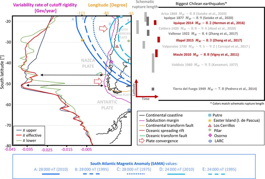
1788                                                                  E. Guillermo Cordaro et al.: Long-term magnetic anomalies

Figure 1. Left side: latitudinal effect of the geomagnetic cutoff rigidity projected over the Chilean convergent margin close to the 70◦ W
meridian. The solid pink lines indicate the edges of tectonic plates. The Nazca Plate is from 18◦ N to 45◦ S in latitude. The South American
continent is on the South American Plate. The Antarctic Plate is from 45 to 79◦ S. The black lines indicate the coastline. In blue are the
iso-values of magnetic intensity due to SAMA proximity. The symbols indicate the stations’ locations. Right: history of Chilean earthquakes.

fect comes from those particles that follow the magnetic field           netic features from disturbances that spread throughout in-
lines, in the turbulent magnetic reconnection that is present            terplanetary magnetic fields. One of those features corre-
in the diurnal variation and the regular variations (Priest and          sponds to the magnetic shielding against incoming turbulent
Forbes, 2000; Kulsrud, 2004; Cordaro et al., 2016; Lazarian              particles which is known as geomagnetic cutoff rigidity Rc
et al., 2020). Other minor irregular magnetic fields such as             (Pomerantz, 1971). The rigidity Rc is defined as the product
auroral events and electric current in the ionosphere are not            of the force of the magnetic field and the curvature radius
considered for this paper (see Diego et al., 2005, for detailed          of the incident particle rg , and it can be estimated globally
description of these phenomena).                                         by using the Tsyganenko magnetic field model (for details
   Some indices are used in order to measure the space dis-              see Smart et al., 2000; Smart and Shea, 2001; Tsyganenko,
turbances and their manifestation in the geomagnetic field.              2002a, b). The Rc variations describe geomagnetic secu-
For example, the Kp index measures the influence of geo-                 lar variations which could be related to geological features
magnetic storms in the horizontal magnetic field (Dieminger              in the Chilean margin (Pomerantz, 1971; Shea and Smart,
et al., 1996), while the Dst index is interpreted as a measure           2001; Smart and Shea, 2005; Herbst et al., 2013; Cordaro et
of the magnetospheric ring-current strength which is propor-             al., 2018, 2019). For example, regarding the latitudinal ef-
tional to the particle’s kinetic energy (e.g., Silva et al., 2017).      fect (Pomerantz, 1971), Cordaro et al. (2019) found that the
Usually, the Dst index can increase by dozens or hundreds of             highest variation rate of effective Rc values were obtained at
nanoteslas during magnetic storms (Kp), which is why it is               46.5◦ S, 76◦ W and at 52◦ S, 76.5◦ W (Fig. 1). The first one
important to incorporate these indices to create reliable mag-           is in the Taitao Peninsula, Chile, which corresponds to the
netic models.                                                            triple junction point of three tectonic plates: Nazca, South
                                                                         American, and Antarctic. The second one is close to Puerto
2.2    Secular variation in the Chilean convergent margin                Natales in the Strait of Magellan area, also a triple junction
                                                                         point of three tectonic plates: South American, Antarctic, and
                                                                         Scotia (Fig. 1). There are other geological and geomagnetic
The magnetic response to these disturbances requires a ref-
                                                                         links such as the flat slab in the Chilean convergent margin
erence model that allows the discrimination of Earth’s mag-

Nat. Hazards Earth Syst. Sci., 21, 1785–1806, 2021                                       https://doi.org/10.5194/nhess-21-1785-2021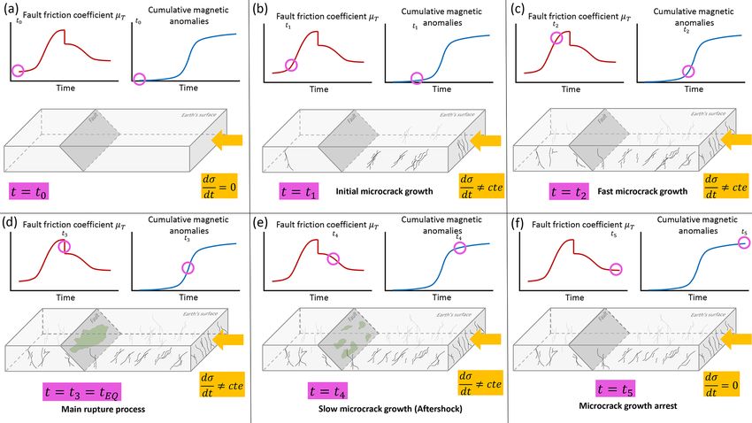
E. Guillermo Cordaro et al.: Long-term magnetic anomalies                                                                      1789

(Cordaro et al., 2018, 2019). However, these results are not         more earthquake-related. The stages correspond to the long-
surprising because changes in Rc represent secular variations        term magnetic evolution, the simple frequency analysis, and
that represent magnetic secular variations created at the outer      wavelet and anomaly analysis. Stations used here are Putre
core (Bloxham et al., 2002; McFadden and Merrill, 2007;              (PUT), Easter Island (IPM, also known as Isla de Pascua),
Sarson, 2007; Finlay, 2007; Herbst et al., 2013). Specifically,      Los Cerrillos (CER), Pilar (PIL), Osorno (OSO), and Labo-
3D models of core mantle boundary (CMB) topology based               ratorio Antártico de Radiación Cósmica (LARC). See Fig. 1
on the velocities of seismic waves (Simmons et al., 2010)            for their locations, and information on PUT, CER, and LARC
show the existence of positive topography in upthrust regions        is in Table 1. In the case of PUT and IPM, the Dobrovolsky
and negative topography in subduction zones (Yoshida, 2008;          area and the earthquake distances will be used in the follow-
Lassak et al., 2010; Soldati et al., 2012). Let us remark that       ing subsections (Table 2).
the intensity of the geomagnetic field within the outer core
is estimated to be of the order of 2–4 mT (rms) (Olson et al.,       3.1   Long-term magnetic records
1999; Olson, 2015), while at the Earth’s surface it varies be-
tween 20 000 and 60 000 nT.                                          A high correlation between the vertical component of the
    The most relevant magnetic feature in the Chilean sector         Earth’s magnetic field and seismic activity at the Putre sta-
is the low magnetic intensity values that correspond to the          tion was found (Cordaro et al., 2018). That is why we seek
influence of the South Atlantic Magnetic Anomaly (SAMA)              to specify this behavior in a shorter time window than the
(e.g., Cordaro et al., 2016). Recently, Tarduno et al. (2015)        period studied previously (1975–2010). In addition, the Bz
argued that SAMA is being created by a topography struc-             component in the Easter Island (IPM) station is also used
ture in the CMB beneath southern Africa. Not only is SAMA            because it has not been thoroughly investigated (note that
linked with global magnetic features such as a geomagnetic           the IPM station was closed in 1968 and subsequently re-
dipole moment (e.g., Heirtzler, 2002; Gubbins et al., 2006),         activated in 2008 by the French INTERMAGNET group
it also corresponds to the closer area between the Earth’s sur-      and the Meteorological Service of Chile) (Chulliat et al.,
face and radiation belt. This proximity allows more charged          2009; Soloviev et al., 2012). The Putre observatory is at
particles and more disturbances in the magnetic field near           18◦ 110 47.8 S, 69◦ 330 10.9 W, 3598 m a.s.l. (meters above sea
the Chilean margin (e.g., Kivelson and Russell, 1995). That          level); and it is located on the western edge of the South
is why a proper magnetic response to external disturbances           American Plate. This zone includes the South Atlantic Mag-
is required before and after earthquake occurrences.                 netic Anomaly (SAMA), the center of which is 1700 km east
                                                                     of this observatory. The measurements confirm low Bz val-
2.3    Magnetic perturbation during seismic events of 27             ues at the station of Putre. The instrument error in the ge-
       February 2010 in Maule, 1 April 2014 in Iquique,              omagnetic measurements is of the order of 5 nT (Cordaro et
       and 16 September 2015 in Illapel                              al., 2012). IPM is located at 27.1◦ S, 109.2◦ W, 82.83 m a.s.l.,
                                                                     on the western edge of the Nazca Plate, characterized as a
The manifestation of a space climate in the geomagnetic field        hotspot (e.g., Vezzoli and Acoocella, 2009). OSO is located
during the periods concerned is defined by the Kp magnetic           at the coordinates 40◦ 200 2400 S, 74◦ 460 6400 W, and PIL is at
activity index as shown in Fig. 2 for the months prior to            31◦ 400 00.000 S, 63◦ 530 00.000 W (Fig. 1).
the three earthquakes: Maule 2010 (12 December 2009 to                  In Putre, a diminution in the values of the whole magnetic
15 March 2010), Iquique 2014 (1 January 2014 to 15 April             field and each of its components is found. This can be at-
2014), and Illapel 2015 (1 July 2015 to 30 September 2015).          tributed to the fact that the Putre observatory is influenced by
For Maule 2010 the magnetic activity reached a Kp index              the South Atlantic Magnetic Anomaly, while on Easter Is-
equal to or greater than 4 on only three isolated occasions,         land the influence of SAMA is weaker (Storini et al., 1999).
and it is therefore considered a calm period; for Iquique            These magnetic influences are also found at the Los Cerril-
2014, activity was concentrated around 19 February 2014,             los observatory. The scientific and technical characteristics
while for Illapel 2015 the maximum activity was recorded             of the Putre (PUT) and Los Cerrillos observatories, i.e., loca-
between 8 and 10 September 2015. In all three cases, activity        tion, altitude, atmospheric depth, type of detectors, geomag-
did not persist in time. In fact, according to Fig. 2, there is no   netic cutoff rigidities, and operating times, may be found in
evidence of an increase in the number of external magnetic           Cordaro et al. (2012, 2016), while for Easter Island (IPM) the
perturbations prior to each earthquake.                              information is available in the SuperMAG network (Chulliat
                                                                     et al., 2009; Gjerloev, 2012). The main characteristics for the
                                                                     observatories, i.e., location, altitude, atmospheric depth, type
3     Main magnetic evolution and frequency analysis                 of detector, and operation time, are shown in Table 1.
                                                                        Measurements of the Bz component are represented in
Magnetic measurements and analysis are presented in this             Fig. 3. We observe similar gradients in Iquique 2014 and Il-
section. The main aim of this section is to use different mag-       lapel 2015 to those found in Maule 2010, giving rise to a
netic methodologies and figure out which of them seems               jump in each case. It is known that these magnetic signals

https://doi.org/10.5194/nhess-21-1785-2021                                  Nat. Hazards Earth Syst. Sci., 21, 1785–1806, 2021
1790                                                              E. Guillermo Cordaro et al.: Long-term magnetic anomalies

Figure 2. The Kp magnetic activity index for the periods prior to the Maule 2010 (a), Iquique 2014 (b), and Illapel 2015 (c) earthquakes
(NOAA SPIDR) (WDCFG, Kyoto University).

are generated by the Earth’s core and disseminated through               For Iquique 2014 the jump recorded in Putre (Fig. 3b) oc-
the mantle, implying changes in the mantle’s electrical con-          curred on 27 December 2013 (solid purple line), a time lapse
ductivity (Stewart et al., 1995).                                     of 96 d before the earthquake (red solid line). A change ap-
   The jump in the Bz component for Maule 2010 was                    pears in the gradient on this date from a diminution of 123 nT
recorded in the Putre station on 23 January 2010 (solid pur-          in the period 14 November 2013 to 27 December 2013 to
ple line in Fig. 3a), a time lapse of 36 d before the earth-          a diminution of 113 nT between 27 December 2013 and
quake (solid red line) and the moment at which a change               15 April 2014; the jump presents a change from −7355 to
appears in the gradient or trend. It alters from a diminu-            −7235 nT, 1 = 120 nT, as shown in Fig. 3. For Iquique 2014
tion of 225 nT in the period of 31 October 2009 to 23 Jan-            the jump measured at IPM occurred on 31 December 2013, a
uary 2010 to a less abrupt diminution of 30 nT between                time lapse of 91 d before the earthquake (Fig. 3c). The trend
23 January 2010 and 3 April 2010; prior to the jump on                shows a slight increase between 30 September 2013 and 3
16 January 2010, there is a small, abrupt diminution from             January 2014, from −19 116 to −19 104 nT, while a further
−5048 to −4927 nT. Discounting this small, abrupt diminu-             slight increase occurs in the period of 3 January 2014 to 6
tion, the 1Bz value between the gradients falls from −4960            May 2014, from −19 101 to −19 099 nT. Note that the size
to −4926 nT, 1 = 34 nT, as shown in Fig. 3a.                          of the jump was −3 nT, as shown in Fig. 4. For Illapel 2015

Nat. Hazards Earth Syst. Sci., 21, 1785–1806, 2021                                    https://doi.org/10.5194/nhess-21-1785-2021

E. Guillermo Cordaro et al.: Long-term magnetic anomalies                                                                               1791

Table 1. The main characteristics for the detectors of Chilean network of cosmic rays and geomagnetic observatories: location, altitude,
atmospheric depth, and types of detector (Cordaro et al., 2012).

   Observatory   Location          Geographical        Altitude     Atmospheric       Instruments (Cordaro et al., 2012)        Time
                                   coordinates         [m a.s.l.]   depth [g/cm2 ]
   Putre         Andes             18◦ 110 47.800 S,   3600         666               Magnetometer, UCLA vectorial flux-        2003–2017
   (PUT)         Mountains,        69◦ 330 10.900 W                                   gate. Muon telescope, three channels.
                 Chile                                                                IGY neutron monitor, three channels,
                                                                                      3 He. UTC by GPS receiver.

   Los Cerril-   Santiago de       33◦ 290 42.200 S,   570          955               Magnetometer, UCLA vectorial flux-        1958–2017
   los (OLC)     Chile, Chile      70◦ 420 59.8100 W                                  gate. Multi-directional muon telescope,
                                                                                      seven channels. Neutron monitor
                                                                                      6NM64, three channels, BF3 . UTC by
                                                                                      GPS receiver.
   LARC          King George       62◦ 120 900 S,      40           980               Magnetometer, UCLA vectorial flux-        1990–2017
                 Island,           58◦ 570 4200 W                                     gate. Neutron monitor 6NM64, six
                 Antarctica                                                           channels, BF3 . Neutron monitor
                                                                                      3NM64, three channels, 3 He. UTC by
                                                                                      GPS receiver.

Figure 3. Vertical component Bz as a function of time at Putre and IPM stations: (a) Maule 2010 at the Putre station, (b) Iquique 2014 at the
Putre station, (c) Iquique 2014 at the Easter Island station, and (d) Illapel 2015 at Easter island station. Trend changes are observed in the
four cases.

the jump measured at IPM occurred on 31 August 2015, a                    ponent at PUT and IPM stations. Fundamental frequencies
time lapse of 16 d before the earthquake. The trend shows a               before these earthquakes ranged from 5.606 to 3.481 µHz or
slight diminution between 31 August 2015 and 20 Septem-                   from one cycle/48.9 h to one cycle/79.13 h (Fig. 4a). The in-
ber 2015, from −19 054 to −19 072 nT, a jump of −11 nT, as                crease in one frequency or a group of frequencies reflects the
one can observe in Fig. 3d.                                               oscillations of the radial magnetic field whose oscillation pe-
                                                                          riod takes from ∼ 2 to ∼ 4 d. Specifically, in the Maule event,
3.2 Simple Fourier analysis                                               peaks for the frequencies 4.747, 5.064, and 5.154 µHz were
                                                                          recorded (blue squares in Fig. 4a). In Iquique peaks of 4.611,
Regarding the frequency analysis, the frequency spectrum                  4.882, and 5.154 µHz were recorded (black dots in Fig. 4a),
values were analyzed for the Maule, Iquique, and Illapel                  and for Illapel, 3.739, 4.630, and 5.520 µHz were recorded
earthquakes using the second derivative of the vertical com-              (red rhombuses in Fig. 4a).

https://doi.org/10.5194/nhess-21-1785-2021                                       Nat. Hazards Earth Syst. Sci., 21, 1785–1806, 2021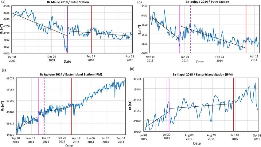
1792                                                                 E. Guillermo Cordaro et al.: Long-term magnetic anomalies

Figure 4. (a) Fast Fourier transformation (FFT) of the second derivative Bz component at Putre station for different events: Maule 2010 and
Iquique 2014. The rise in frequencies in the range of microhertz are compared to the FFT of the second derivative at IPM station for Illapel
2015. (b) FFT every 15 d for Iquique 2015 at the Putre magnetometer. (c) FFT every 8 d for Illapel 2015 at the Easter Island magnetometer.

Table 2. The maximum radius where the ionosphere–lithosphere–           tributed to space weather in the daily average measurements.
atmosphere coupling may affect magnetic measurements corre-             According to Cordaro et al. (2018), the magnetic field’s ver-
sponding to each earthquake studied at the stations of Putre and        tical component showed variations related to the Maule 2010
IPM (Dobrovolsky et al., 1979; Pulinets and Boyarchuk, 2004).           earthquake. That is why values of the vertical component of
The preparation area or Dobrovolsky area is defined by the ra-          the geomagnetic measurements at the OSO station were con-
dius r = 100.43M , where M is the earthquake magnitude. This table
                                                                        sidered. Note that the OSO station is the closest station to the
shows that the Putre and IPM stations are within the earthquake
preparation stage for Maule, Iquique, and Illapel.
                                                                        main earthquake. In order to avoid space weather influence,
                                                                        the highest variations were not considered. One way to con-
 Event           Magnitude     Radius r    Station distance
                                                                        sider these two restrictions is by using statistical analysis.
                     [Mw ]        [km]     from earthquake [km]         For example, a lower and upper threshold could be defined
                                                                        by using the standard deviation. Consider the higher mag-
 Maule 2010              8.8     ∼ 6100    Putre ∼ 2030                 netic peaks, but they are not too meaningful because they
 Iquique 2014            8.2     ∼ 3360    Putre ∼ 300
                                                                        could be related to space weather conditions. An example of
 Illapel 2015            8.3     ∼ 3700    IPM ∼ 3700
                                                                        this statistical analysis when an upper threshold of 2 standard
                                                                        deviations is used can be found in Fig. 5, in which panels
                                                                        (a), (b), and (c) represent the Maule 2010, Iquique 2014, and
   In order to identify a temporal domain where these fre-              Illapel 2015 earthquakes, respectively. For Maule 2010, the
quencies arise, FFT is applied every 20 d as a first approx-            spectral analysis shows a dramatic increase 30 d before the
imation (Fig. 4b, c). Before the Iquique 2014 event a jump              Maule earthquake and a decrease 10 d after the earthquake
in intensity was observed that was associated with the fre-             occurrence (yellow and green arrows in Fig. 5a). The fre-
quency of 5.154 µHz for the period 27 December 2013 to                  quencies that rise comprise a range close to 3–5 µHz. Note
11 January 2014, i.e., after the jump (Figs. 3b, 4b). Similar           that no other significant increase is seen during the 2 years of
frequencies (3.739 µHz) rise during 1 to 8 September 2015               measurements between days −365 up to −30, and between
before the Illapel 2015 event (Fig. 4c). These findings imply           days 10 and 365 it is clear that there is no significant rise
a more detailed methodology is required in order to study the           in frequencies (blue shading in Fig. 5a). Panel (b) of Fig. 5
origin of these frequencies.                                            shows the results for Iquique 2014, which is characterized
                                                                        by two peaks. The first one rises 89 d before the earthquake
3.3    Wavelet analysis
                                                                        (yellow arrow in Fig. 5b), while the second one occurs af-
We have used the wavelet transformation to analyze local-               ter the Iquique earthquake (after the red line, which indicates
ized versions of power within a geomagnetic time series. In             the earthquake day). The Illapel case is also characterized by
this way, it can break down a time series into time–frequency           two peaks, as shown in panel (c) of Fig. 5. The first rise oc-
space and determine the dominant modes of variability and               curs ∼ 159 d before the earthquake (yellow arrow in Fig. 5c),
how they vary over time (Torrence and Compo, 1998). Here,               while the second rise is 52 d before the main earthquake (grey
the goal is to look for the rare variations that could not be at-       arrow in Fig. 5c). Despite this promising methodology that

Nat. Hazards Earth Syst. Sci., 21, 1785–1806, 2021                                       https://doi.org/10.5194/nhess-21-1785-2021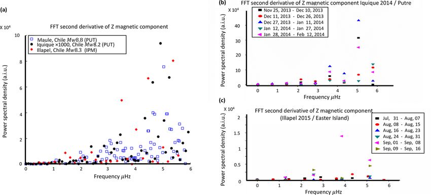
E. Guillermo Cordaro et al.: Long-term magnetic anomalies                                                                           1793

Table 3. Days before and after each frequency or anomaly rise for each earthquake considered (Maule 2010, Iquique 2014, Illapel 2015, and
Mexico (Puebla) 2017 for anomalies).

                                                      Rise in frequencies
                                         Wavelet                            Spectrogram
              Event               Days before       Days after       Days before       Days after           Rise in cumulative
                                   earthquake      earthquake         earthquake      earthquake         anomalies, days before
                              (secondary rise)                   (secondary rise)                   earthquake (secondary rise)
              Maule 2010               ∼ 30              ∼ 10             ∼ 48              ∼ 64                   ∼ 46 (∼ 21)
              Iquique 2014             ∼ 89              ∼ 44      ∼ 191 (∼ 95)             ∼ 32                         ∼ 83
              Illapel 2015      ∼ 159 (∼ 52)              ∼2              ∼ 41              ∼ 41                         ∼ 60
              Mexico 2017                  –                –                 –                –                   ∼ 67 (∼ 42)

considers the daily average and the upper threshold, an im-                 other researchers have used cubic splines instead of mov-
proved implementation of physical (i.e., space weather con-                 ing averages (e.g., De Santis et al., 2017). In our case we
ditions) and statistical (adequate definition of anomalies and              use a = 0.07, b = 0.25, and c = 0.5–2a. The uncertainty in
frequency considerations) analysis is required.                             the fluxgate magnetometers (SuperMAG) from OSO and PIL
   Finally, let us point out that more profound and sophisti-               stations is δBi = ±0.1 nT, while the error in the moving av-
cated multiresolution wavelet analysis on time series related               erage implementation is δ B̄i = ±0.1 nT. As residual values
to earthquakes has been performed by Telesca et al. (2004,                  are defined as the difference between real and smoothed data
2007). This kind of study will be considered in future works.               (1Bi = Bi − B̄i ), the total error propagation of the residual
                                                                            is δBi + δ B̄i = ±0.2 nT.
3.4     Anomaly analysis                                                       Let us comment that the error in propagation is used to
                                                                            define a threshold that determines when a residual is con-
In order to identify and discriminate external variations from              sidered anomalous or not. For instance, in statistics 0.6745σ
those that could be considered lithospheric (variations with                represents the 50 % of the data that are closer to the average
lithospheric origin), this subsection handles the definitions               (where σ is the standard deviation). This means that residuals
of anomalous variations. This definition will be obtained                   less than 0.6745σ nT are closer to the average and therefore
considering the external perturbation by using the Dst in-                  are more common. As residuals are considered anomalous
dex (http://wdc.kugi.kyoto-u.ac.jp, last access: 7 June 2021).              when they are unlikely, anomalous data should be defined as
Then spectral analysis will be performed. Additionally, the                 those residuals larger than 0.6745σ nT. By adding the error
data used in this subsection are standard and come from the                 propagation as a condition (0.6745σ + 0.2 nT) and consider-
SuperMAG network (http://supermag.jhuapl.edu/, last ac-                     ing that the standard deviation is similar to σ ∼ 0.1 nT, the
cess: 7 June 2021). The data have a sampling frequency of                   percentage of residuals that meets this condition is consider-
one datum per minute, and a period of 1 year before and                     ably smaller than the 50 % of the data (less common). Thus,
1 year after each earthquake was chosen.                                    residuals 1Bi are considered anomalous (1Bai ) when
                                                                            |1Bi | ≥ 0.6745σ + 0.2 nT.                                 (1)
3.4.1    Magnetic threshold definition
                                                                            The vertical magnetic thresholds found are 0.2246995 nT at
In the method of cumulative magnetic anomalies on the sur-                  OSO (27 February 2009–27 February 2011), 0.2362868 nT
face of Earth, we used statistically atypical or anomalous                  at PIL (1 April 2013–1 April 2015), and 0.2352825 nT at
values, that is, data that are quite far from the average val-              PIL (16 September 2014–16 September 2016). These thresh-
ues of the sample. So, we compare real values of Bi with a                  old are ∼ 6, ∼ 4.5, and ∼ 4.5 times larger than each respec-
more representative value of the sample, its average B̄i . We               tive σ . This means that each anomaly above this threshold
will call the difference between the two the magnetic residual              meets the 3σ criterion (a valid observation). Furthermore,
1Bi . By using the distribution of data, we can define when                 the thresholds are close to the 5σ criterion which corre-
a value is atypical or anomalous in a normal distribution by                sponds to the standard discovery criteria in the physical sci-
statistical definitions of quartiles and outliers.                          ences; for example this criterion was used in the discovery
   On the one hand, we create a filter that eliminates the                  of the Higgs boson (https://home.cern/news/news/physics/
frequencies averaged near Nyquist and establishes a filter                  higgs-within-reach, last access: 7 June 2021).
that eliminates high frequencies (stochastic filter). The op-                  Regarding the external contribution, the data considered
tion was to consider a weighted moving average of five                      are for quiet periods, |Dst|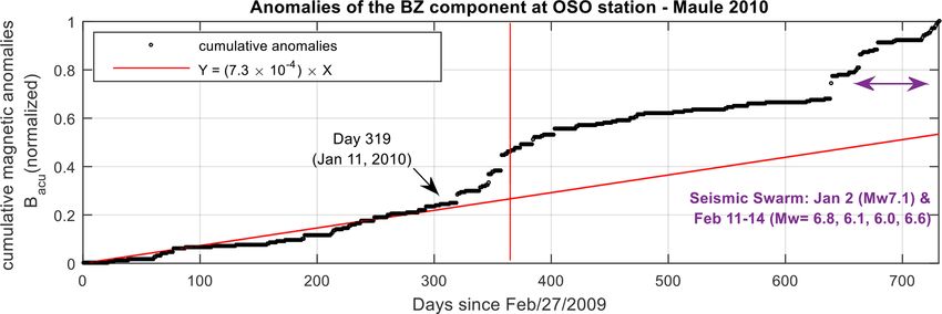
1794 E. Guillermo Cordaro et al.: Long-term magnetic anomalies
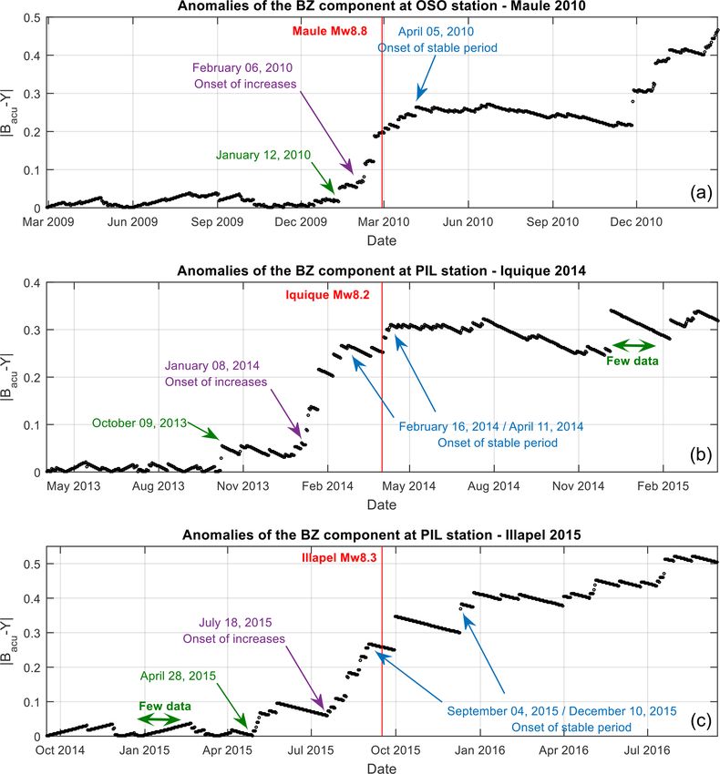
Figure 5. Wavelet for Bz at OSO station is shown. These graphs are obtained by restricting the peaks considered in a band and daily
average values during 2 years of measurements. The wavelet spectrum shows an increase prior to and after the Maule earthquake. Unlike the
spectrogram method where it is enough to consider the anomalous peaks above a threshold, wavelet analysis is more complex to calibrate
than spectrogram analysis (upper limit).
(Hitchmn et al., 1998). Some researchers who have used as Pday ≈ 0.0014. Contrarily, if 1 single day shows, let us
30
satellites consider only the time periods in which the Dst say, 30 anomalies, the probability is P30 = Pday ∼ 10−86 .
index is less than or equal to 20 nT (e.g., Marchetti and This means that the occurrence of 30 anomalies is virtually
Akhoondzadeh, 2018) or equal to 10 nT (e.g., De Santis et zero, and it could imply that the previous filters (anomaly
al., 2017). That means that the space weather conditions definition, Dst, and quiet time) failed during that day. Then,
could invalidate the anomaly condition defined in Eq. (1) it is not possible to consider those days where the number of
if |Dst|>10 nT. Then, the proper application of Eq. (1) is anomalies per day is considerably larger than 2. That is why
linked to those times where space weather activity is low. days with more than 10 anomalies are not considered valid.
That is when |Dst|E. Guillermo Cordaro et al.: Long-term magnetic anomalies 1795
lap, which corresponds to a reasonable spectral and time res-
olution (see Rabiner and Schafer, 1980, and Oppenheim et
al., 1999, for spectrogram theory and application). The OSO
and PIL spectrograms for Maule 2010, Iquique 2014, and Il-
lapel 2015 are shown in Fig. 6.
In the Maule 2010 event, the spectrogram of the vertical
magnetic component at the OSO station is shown in Fig. 6a.
There is no significant rise in frequencies during the period
before the Maule event (before ∼ 10 January 2010). Never-
theless, a dramatic increase during the period 10 January–2
May 2010 occurs. Specifically, the rise in frequencies lies in
the range ∼ 1–2.2 mHz. The onset of this rise (10 January)
occurs more than 1 month before the Maule earthquake (27
February) and lasts almost 4 months. That means that the
spectral density reduces their activity after ∼ 2 months of the
earthquake.
The spectrogram for Iquique 2014 is characterized by two
peaks (Fig. 6b). The first one corresponds to 22 September
2013, and the second one corresponds to ∼ 8 March 2014.
Here, the frequency range comprises between ∼ 1.2 and
2.7 mHz, which is similar to that found in the Maule spectro-
gram. However, the main peak occurred during March, which
is characterized by a dominant frequency close to 2.5 mHz,
while the dominant frequencies in Maule 2010 are close to
1.2 and 2.2 mHz. There is an additional difference compared
to the Maule event: the rise in frequencies in Iquique 2014
comprises a significant decrease (or “valley”) in the spec-
tral density, which lasts almost 2 months (∼ 9 November–27
December 2013). It means that the second rise in frequen-
cies lasts more than 4 months (∼ 27 December 2013–3 May
2014), which is a similar duration compared to the frequency
rise of Maule 2010.
The final spectrogram is found in Fig. 6c, which corre-
sponds to the Illapel 2015 event. Here, it can be seen that al-
most the entire period was characterized by close-to-zero fre-
quency variations. Nevertheless, the frequency rise is similar
to that obtained in Maule 2010. That is, significant frequen-
cies rise only on dates close to the earthquake event. The rise
lasts almost 3 months (∼ 6 August–27 October 2015). It is
important to note that the gap in September 2015 is due to the
strong spatial weather activity. Despite this, it is clear that the
earthquake occurrence is during periods of high-frequency
activity, which is a similar feature compared to Maule 2010
and Iquique 2014. Figure 6. Spectrogram analysis of vertical magnetic components
Panels (a)–(c) of Fig. 6 show that three strong earthquakes after the external influence is filtered. (a) The rise in a range of fre-
(Maule 2010, Iquique 2015, and Illapel 2015, respectively) quencies (1–2.5 mHz) appears prior to and after the Maule 2010
occurred during the rise in ultra-low frequencies of the ver- earthquake (OSO station). The active frequencies last less than
tical magnetic component. It is important to highlight that 3 months. (b) The rise in similar frequencies appears prior to the
these frequencies (mainly 1–2.5 mHz) vanish or reduce their Iquique 2014 earthquake in the vertical component of the PIL sta-
intensity values during other time periods. This is in agree- tion. This frequency activity lasts more than 5 months. (c) The solar
ment with other authors who have claimed that accompany- events are intense during September 2015. Nevertheless, this can be
seen as an increase in the spectrum since August 2015. This fre-
ing ultra-low frequencies (e.g., Contoyiannis, et al., 2016;
quency activity lasts close to 3 months. Three earthquakes hit when
Han et al., 2020) and the increases in the number of magnetic the rise in ultra-low frequencies (mHz) exists. Note that Iquique is
anomalies are related to the earthquake preparation process not filtered by Dst as Maule and Illapel are.
(e.g., De Santis et al., 2017). It means that anomalous peaks
https://doi.org/10.5194/nhess-21-1785-2021 Nat. Hazards Earth Syst. Sci., 21, 1785–1806, 20211796 E. Guillermo Cordaro et al.: Long-term magnetic anomalies
produce the magnetic oscillations in the magnetic records. in Maule, Iquique, and Illapel, which is similar behavior to
By following the Venegas-Aravena et al. (2019) findings, the that recorded in the Mexico earthquake (Fig. 9; Marchetti
number of these peaks should also increase (decrease) in time and Akhoondzadeh, 2018). This indicates that anomaly be-
before (after) earthquake occurrences. havior could correspond to a lithospheric origin. Currently,
it has been shown that the origin of these anomalies is as-
3.4.3 Cumulative daily anomalies sociated with the cracking (or microcracking) of the semi-
fragile–ductile part of the lithosphere (crust) due to changes
By following the anomaly definition (Sect. 3.4.1), it is pos- in stress (Venegas-Aravena et al., 2019). Typically, strain
sible to find the daily number of anomalies. For example, appears when solids undergo loads or stress accumulation.
in Fig. 7 the case of the OSO station is shown. Black dots However, microcracks rise specifically when solids cannot
follow a stable linear increase in the number of cumulative contain more deformation and prior to the main failure (e.g.,
anomalies (red line). Nevertheless, this tendency breaks close Stavrakas et al., 2019; Li et al., 2020). Experimentally, it
to 11–12 January 2010. From those days up to the first week has been shown that these conditions break the electrical
of April, the numbers of anomalies experiences a dramatic neutrality within materials and generate an electrical flux
increase. In the middle of this increase, the Maule earthquake through rocks in a process known as pressure-stimulated cur-
hits (27 February 2010). By subtracting the initial linear ten- rents or PSCs (e.g., Anastasiadis et al., 2004). Furthermore,
dency and comparing it to the PIL station (Iquique 2014 and it has been shown that PSCs can explain that the fractal na-
Illapel 2015), the sigmoidal feature is clearer (Fig. 8). The ture of cracks is sufficient to generate the frequency spec-
anomalies start to increase prior to each earthquake. For ex- trum, co-seismic variations, anomalies and their behavior,
ample, this increase started ∼ 47 d before the Maule 2010 and variation in the ionosphere in a theory known as seismo-
earthquake, ∼ 90 d before the Iquique 2014 earthquake, and electromagnetic theory (Venegas-Aravena et al., 2019). Re-
∼ 60 d before the Illapel 2015 earthquake (Fig. 8). garding the time evolution of magnetic anomalies, De Santis
Other researchers have used very different implemen- et al. (2011) have shown that the sigmoidal shape is due to
tations, definitions, methodologies, and data in order a manifestation of the stress changes when it reaches a criti-
to find these anomalies. For example, Marchetti and cal point. Nowadays, theoretical development, geodynamical
Akhoondzadeh (2018) have also found a sigmoidal signature measurements, and experimental studies have shown that the
in the anomalies of the Y components recorded by different sigmoidal shape appears as a consequence of the dramatic
satellites for the Mexico (Puebla) 2017 earthquake. In order increase in the number of microcracks (at a depth of a few
to compare Mexico 2017 with Maule 2010, Iquique 2014, tens of kilometers) prior to the main earthquake ruptures (De
and Illapel 2015, the initial linear trend has been removed Santis et al., 2015; Stavrakas et al., 2019; Venegas-Aravena,
(Fig. 9). The initial onset of anomalies increased close to 60 d et al., 2019).
prior to the Mexico 2017 earthquake. Note that in the four A schematic representation of the crack generation in the
cases, the sigmoidal features are almost the same: a linear geodynamical context can be seen in Fig. 10. At the ini-
stable number of anomalies characterize the initial period. tial time t = t0 , the intact lithosphere undergoes a uniaxial
Then a dramatic increase in the number of daily anomalies non-constant stress σ (Fig. 10a). Then the first signs of mi-
is followed by the main earthquake. This time is different in crocracks appear at t = t1 due to the increase in the stress
each earthquake but it lies between 50–90 d after the initial (Fig. 10b). When the lithosphere cannot withstand more de-
anomalies increase. After the seismic events happen, the cu- formation, a dramatic increase in the crack generation ap-
mulative numbers do not behave similarly. For example, in pears throughout the lithosphere (t = t2 in Fig. 10c). At
the Mexico 2017 earthquake, the anomalies remain stable, this point (t = t3 in Fig. 10d), the crack generation is not
while in the Maule 2010 earthquake they still increase but sufficient to release the excess of uniaxial stress. Then the
in a less dramatic manner. At the end of the OSO measure- lithosphere cannot release energy by either deformation or
ments, several anomalies appear, but it is not clear whether the crack generation mechanism. That is why the rupture
these events could be related to other seismic events. In order (earthquake) occurs (green area in Fig. 10d) at t = t4 . After
to understand the physics that lies in these events, a theoreti- the main rupture, another aftershock occurs (smaller green
cal mechanism is required. patches within the fault in Fig. 10e). Nevertheless, the num-
ber of anomalies starts to decrease. Finally, the microcrack
generation stops because the deformation is sufficient to han-
4 Magnetic anomalies and fracture mechanics by dle the lithospheric response to non-constant uniaxial stress
considering the seismo-electromagnetic theory (Fig. 10f).
Additionally, Venegas-Aravena et al. (2019) found that
The frequency analysis (Figs. 5, 6) and cumulative number the increase in the number of anomalies is controlled by
of magnetic anomalies (Figs. 7, 8, 9) show an increase (spec- the same fractal nature that drives the microcrack genera-
tral intensity and anomalies number) before each earthquake tion. This means that the frequency of the electrical flux
occurs. In the anomalies case, a clear sigmoidal feature rises could cover several magnitude orders. For example, Figs. 4,
Nat. Hazards Earth Syst. Sci., 21, 1785–1806, 2021 https://doi.org/10.5194/nhess-21-1785-2021E. Guillermo Cordaro et al.: Long-term magnetic anomalies 1797 Figure 7. Accumulated magnetic anomalies of Bz and a linear interpolation in the period of 2 years starting on 27 February 2009. The data were taken at the OSO station. Close to the main earthquake, the linear trend breaks and the number of anomalies increases. Other important seismic events hit near the stations during the last period. Nevertheless, it is not clear that the anomaly increases are due to these specific events. Figure 8. Variation in the accumulated diary of magnetic anomalies of Bz during 2 years close to the three earthquakes: (a) Maule, (b) Iquique, and (c) Illapel. The data were taken at OSO station (a) and PIL station (b, c), respectively. Is clear that the sigmoidal shape is similar in all of the earthquakes. This means that these stations recorded a dramatic increase in the number of magnetic anomalies between 50 and 90 d prior to each earthquake. https://doi.org/10.5194/nhess-21-1785-2021 Nat. Hazards Earth Syst. Sci., 21, 1785–1806, 2021
1798                                                                E. Guillermo Cordaro et al.: Long-term magnetic anomalies

Figure 9. (a) Accumulated diary of magnetic anomalies during 2 years, in component Y from 1 April to 15 October 2017 for the Mexico
earthquake of 8 September 2017, Mw 8.2. (b) Residual behavior of Mexico earthquake. The data are open source and were taken from
the swarm project (https://swarm-diss.eo.esa.int/, last access: 7 June 2021). Methodology was developed by Marchetti and Akhoondzadeh
(2018).

Figure 10. Schematic representation of the seismo-electromagnetic theory. The anomalies generation are owing the creation of several
microcracks. The number of cracks increase because the internal collapse of the lithosphere when a non-constant uniaxial stress is applied.

Nat. Hazards Earth Syst. Sci., 21, 1785–1806, 2021                                      https://doi.org/10.5194/nhess-21-1785-2021
E. Guillermo Cordaro et al.: Long-term magnetic anomalies                                                                  1799

5, and 6 are characterized by the rise in different frequen-     are notorious, which is why a first approach using frequency
cies (micro- to millihertz), which are known as ultra-low        analysis was made.
frequency (ULF), prior to the main earthquakes. These fre-          Specifically, significant frequency data obtained for the
quency ranges were also found and described in other re-         Maule 2010 earthquake, Chile; the Tōhoku 2011 earthquake,
search such as that of Fenoglio et al. (1995), Vallianatos and   Japan; and the Sumatra–Andaman 2004 earthquake, Indone-
Tzanis (2003), Fraser-Smith (2008), De Santis et al. (2017),     sia, range from 4.747 to 5.154 µHz, from 4.747 to 5.606 µHz,
and Cordaro et al. (2018).                                       and from 3.481 to 5.425 µHz, respectively (Cordaro et al.,
   Finally, it has been concluded that there must be precur-     2018). These fundamental frequencies were detected before
sory magnetic anomalies of the order of 0.1 nT related to        the earthquakes in the areas of the Pacific Ocean in the
earthquakes on the Earth’s surface (e.g., De Santis et al.,      Southern Hemisphere and the Eurasian (2011) and Philippine
2017; Chernogor, 2019; Venegas-Aravena et al., 2019). In         (2004) areas in the Northern Hemisphere. Now these signifi-
the previous section, it was found that the minimum value to     cant frequencies have been obtained again in different places
define an anomaly was close to 0.2 nT. Therefore, this exper-    and at different times on Earth: for Iquique 2014, peaks of
imental result is in agreement with the theoretical value ob-    4.611, 4.882, and 5.154 µHz and for Illapel 2015, peaks of
tained. Consequently, as the seismo-electromagnetic theory       3.739, 4.630, and 5.520 µHz (Fig. 4). Up to this point, the
indicates, those magnetic anomalies may have a lithospheric      rise in these frequencies could be thought of as normal mag-
origin. Furthermore, the behavior of all these anomalies fea-    netic behavior with a high degree of coincidence. That is why
tures a preceding increase similar to that of other seismic      other methodologies were used in order to clarify the origin
events that use different data and methods (e.g., De Santis      of these frequencies.
et al., 2019a, 2019b, and references therein).                      In order to avoid bias or technical malfunction, we have
                                                                 decided to use different stations that belong to an interna-
                                                                 tional network with open-source data (SuperMAG). These
5   Discussions and conclusions                                  stations (OSO and PIL) were the closest to the three earth-
                                                                 quakes that had continuous measurements. The time period
The most significant characteristics of the magnetic field and   was 1 year before each earthquake and 1 year after, giv-
its variations are found in the z component, which we have       ing 6 years of combined measurements where the frequency
observed and recorded at the Putre and IPM observatories.        sample was one datum per minute.
The previous measurements show that there is evidence of a          The first approach was performed by using wavelet anal-
progressive increase in the phenomenon known as the South        ysis at the OSO station. Here, in order to avoid normal vari-
Atlantic Magnetic Anomaly (SAMA) (Cordaro et al., 2019).         ations and external perturbation, daily average values were
As expected, it generates a significant deviation in the in-     performed by imposing a lower and upper restriction be-
tensities present in the OP station as shown in the magnetic     fore applying wavelet analysis. Fig. 5a shows the increase in
iso-values (Fig. 1). Combining this information with data        the frequency range (>2 µHz) ∼ 30 d before the Maule 2010
from the IPM station, the behavior of the radial component of    earthquake. These frequency activities last for up to ∼ 10 d
the geomagnetic field for the three most significant seismic     after the earthquake. Similar frequency results were obtained
events in the Chilean Pacific sector during the period 2010–     for Iquique 2014 (Fig. 5b) and Illapel 2015 (Fig. 5c). De-
2015 was recorded, and it corroborates the magnetic relation     spite the abovementioned results, the previous restrictions
with seismology shown in Potirakis et al. (2016), Contoyian-     might be seen as arbitrary. That is why we moved to a
nis et al. (2016), and De Santis et al. (2017), who used other   stricter, stronger, and bias-free methodology. Besides, three
methods.                                                         facts should be taken into account. The first one is consid-
   The normal magnetic trend showed some long-term varia-        ering the physics-based filter processes, which remove most
tions. For example, there were breaks in the trend or a jump     of the noise and external disturbances. Thus, this allows per-
in Bz , followed by a time lapse and seismic movement as         forming more simple frequency analysis such as the moving
one can observe in Fig. 3. These jumps occur in different        Fourier transform (spectrogram). The second one is the tridi-
forms: in Putre they are significant, reaching values of tens    mensional representation. This is important because it is pos-
of nanoteslas, while in IPM the jump is barely 10 nT. The        sible to observe the relative frequency intensity differences in
time lapse between each jump and the seismic event differs       a reliable way. Furthermore, the third one is that this spectro-
in each event. For Maule 2010 it was 36 d; for Iquique 2014      gram and its tridimensional representation allow us to com-
it was 96 d, and for Illapel it was 16 d. This time difference   pare our results to previous works in the field (for example,
may be due to an important factor: it appears that the jump is   Cordaro et al., 2018).
not equally strong in the three events, since the jump before       The definition of magnetic anomalies was given in
the Iquique 2014 event was considerably weaker than the          Sect. 3.4.1. There the anomalous magnetic variations were
one before Illapel 2015 and preceded the event by a longer       defined by using statistical analysis. That is, one variation or
time lapse (96 d). The more abrupt jump recorded in Illapel      peak will be considered anomalous if it reaches values be-
was followed by a shorter time lapse (16 d). These changes       yond a certain threshold, a threshold that is defined by the

https://doi.org/10.5194/nhess-21-1785-2021                              Nat. Hazards Earth Syst. Sci., 21, 1785–1806, 2021
You can also read