The regional impact of urban emissions on air quality in Europe: the role of the urban canopy effects
←
→
Page content transcription
If your browser does not render page correctly, please read the page content below

Atmos. Chem. Phys., 21, 14309–14332, 2021
https://doi.org/10.5194/acp-21-14309-2021
© Author(s) 2021. This work is distributed under
the Creative Commons Attribution 4.0 License.

The regional impact of urban emissions on air quality in Europe:
the role of the urban canopy effects
Peter Huszar1 , Jan Karlický1,3 , Jana Marková1,2 , Tereza Nováková1 , Marina Liaskoni1 , and Lukáš Bartík1
1 Department   of Atmospheric Physics, Faculty of Mathematics and Physics, Charles University, Prague,
V Holešovičkách 2, 18000, Prague 8, Czech Republic
2 Czech Hydrometeorological Institute (CHMI), Na Šabatce 17, 14306, Prague 4, Czech Republic
3 Institute of Meteorology and Climatology, Department of Water, Atmosphere and Environment, University of Natural

Resources and Life Sciences, Vienna, Gregor-Mendel-Straße 33, 1180 Vienna, Austria

Correspondence: Peter Huszar (peter.huszar@mff.cuni.cz)

Received: 28 April 2021 – Discussion started: 3 June 2021
Revised: 2 September 2021 – Accepted: 7 September 2021 – Published: 27 September 2021

Abstract. Urban areas are hot spots of intense emissions, and   showed that if UCMF is included, the UEI of these pollu-
they influence air quality not only locally but on a regional   tants is about 40 %–60 % smaller, or in other words, the ur-
or even global scale. The impact of urban emissions over        ban emission impact is overestimated if urban canopy effects
different scales depends on the dilution and chemical trans-    are not taken into account. In case of ozone, models due
formation of the urban plumes which are governed by the         to UEI usually predict decreases of around −2 to −4 ppbv
local- and regional-scale meteorological conditions. These      (about 10 %–20 %), which is again smaller if UCMF is con-
are influenced by the presence of urbanized land surface via    sidered (by about 60 %). We further showed that the impact
the so-called urban canopy meteorological forcing (UCMF).       on extreme (95th percentile) air pollution is much stronger,
In this study, we investigate for selected central European     and the modulation of UEI is also larger for such situations.
cities (Berlin, Budapest, Munich, Prague, Vienna and War-       Finally, we evaluated the contribution of the urbanization-
saw) how the urban emission impact (UEI) is modulated           induced modifications of vertical eddy diffusion to the mod-
by the UCMF for present-day climate conditions (2015–           ulation of UEI and found that it alone is able to explain the
2016) using two regional climate models, the regional cli-      modeled decrease in the urban emission impact if the effects
mate models RegCM and Weather Research and Forecasting          of UCMF are considered. In summary, our results showed
model coupled with Chemistry (WRF-Chem; its meteorolog-         that the meteorological changes resulting from urbanization
ical part), and two chemistry transport models, Comprehen-      have to be included in regional model studies if they intend to
sive Air Quality Model with Extensions (CAMx) coupled to        quantify the regional footprint of urban emissions. Ignoring
either RegCM and WRF and the “chemical” component of            these meteorological changes can lead to the strong overesti-
WRF-Chem. The UCMF was calculated by replacing the ur-          mation of UEI.
banized surface by a rural one, while the UEI was estimated
by removing all anthropogenic emissions from the selected
cities.
   We analyzed the urban-emission-induced changes in near-      1   Introduction
surface concentrations of NO2 , O3 and PM2.5 . We found
increases in NO2 and PM2.5 concentrations over cities by        Already more than 50 % of the human population lives in ur-
4–6 ppbv and 4–6 µg m−3 , respectively, meaning that about      ban areas, and an increase over 60 % during the upcoming
40 %–60 % and 20 %–40 % of urban concentrations of NO2          decades is foreseen (UN, 2018). The consequences of urban-
and PM2.5 are caused by local emissions, and the rest is        ization (i.e., the transition from rural to urban surfaces) on
the result of emissions from the surrounding rural areas. We    atmospheric conditions are evident (Folberth et al., 2015),
                                                                and they affect both the climate (Zhao et al., 2014; Zhu et al.,

Published by Copernicus Publications on behalf of the European Geosciences Union.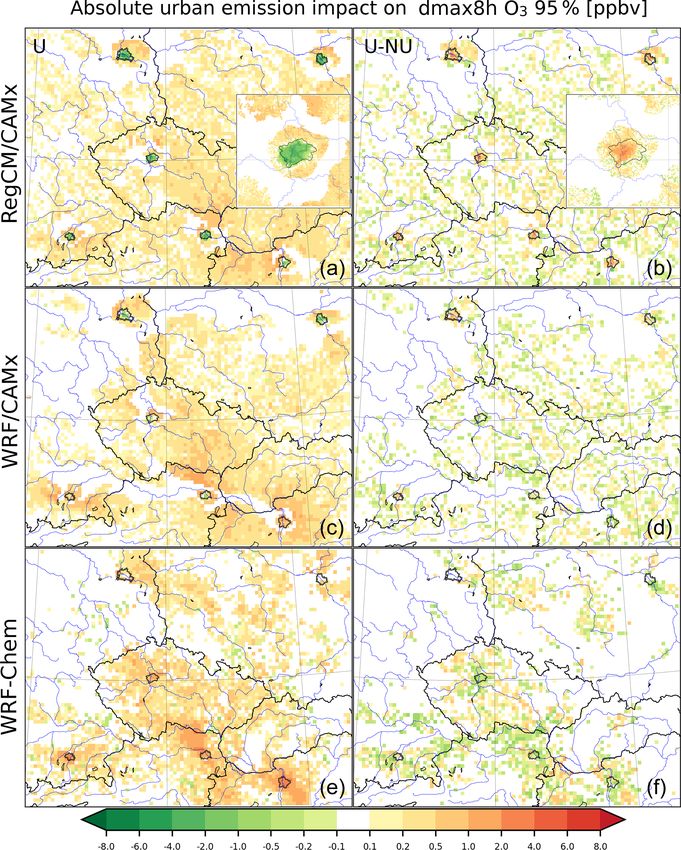
14310                                                               P. Huszar et al.: The regional impact of urban emissions

2017; Huszar et al., 2014; Karlický et al., 2018, 2020) and         precursor for sulfate aerosol (PSO4 ) formation is SO2 . Al-
air pollution (Freney et al., 2014; Timothy and Lawrence,           though SO2 emissions over the last decades have decreased
2009; Butler and Lawrence, 2009; Im and Kanakidou, 2012;            globally (Zhong et al., 2020), the significant perturbation of
Huszar et al., 2016a), as well as the possible interactions be-     aerosol burden is found in many urbanized regions (Gut-
tween them (e.g., Huszar et al., 2018b, 2020a; Han et al.,          tikunda et al., 2003; Yang et al., 2011). Apart from affecting
2020; Fan et al., 2020) that often lead to complex counteract-      photochemistry, emissions of NOx lead to the formation of
ing effects (Yu et al., 2020).                                      nitrate aerosol (PNO3 ). If the meteorological conditions are
   In principle, cities influence the physical and chemical         favorable, NOx from cities can enhance background PNO3
state of the atmosphere via two primary pathways. First of          levels significantly (Lin et al., 2010). Ammonia (NH3 ), al-
all, urban canopies are covered by artificial materials and ob-     though not emitted largely by cities, is an efficient contribu-
jects in a specific geometric layout (building and streets) re-     tor to the formation of sulfate and nitrate aerosol (by form-
sulting in a range of effects on the meteorological conditions      ing ammonium sulfates and ammonium nitrates), and its im-
– i.e., they act via the so-called urban canopy meteorologi-        portance in connection with city emissions is highlighted
cal forcing (UCMF) as defined by Huszar et al. (2020a). In          in many studies (e.g., Behera and Sharma, 2010, and ref-
particular, temperature is increased in cities due to the urban     erences therein). In general, the thermodynamic system of
heat island (UHI) effect (Oke, 1982; Oke et al., 2017). Due to      ammonium-sulfate–nitrate–water solution is rather compli-
enhanced roughness, the city-scale wind speed is decreased          cated, and its equilibrium state is highly dependent on the
(Huszar et al., 2014; Jacobson et al., 2015; Zha et al., 2019),     initial ratio (emission) of SO2 –NOx –NH3 and the prevail-
while for turbulence (especially the vertical eddy diffusivity)     ing meteorological conditions (Martin et al., 2004); thus high
a strong increase is seen (Barnes et al., 2014; Huszar et al.,      variability in the contribution of different cities to aerosol is
2018b, 2020a; Ren et al., 2019). Secondly, due to high pop-         expected. Apart from the SIA, directly emitted organic and
ulation density and thus concentrated human activities and          elemental carbon (OC and EC) can also be a major fraction
energy demand, cities represent an intense source of both           of the urban aerosol impact, as shown, for example, for Paris
greenhouse (Folberth et al., 2012) and short-lived pollutants       by Freney et al. (2014).
that impact not only the local air quality but act on a re-            As the dilution of urban plumes into larger scale includes
gional scale (Freney et al., 2014; Panagi et al., 2020) or even     its mixing with rural emissions and the formation of sec-
a global one (Butler and Lawrence, 2009).                           ondary pollutants, its atmospheric footprint requires com-
   Indeed, cities emit large quantities of different pollutants     plex modeling experiments in which both gas phase and
with various chemical characteristics. They encompass the           aerosol chemistry and transport are simultaneously consid-
emissions of oxides of nitrogen (NOx ) emitted mainly by            ered and coupled to meteorological conditions. Indeed, nu-
road transportation along with non-methane volatile organic         merous modeling studies attempted to evaluate the impact
compounds (NMVOCs). Depending on their ratio, the photo-            of urban emissions at different scales. On a global scale,
chemical regime in and around cities is determined as being         the urban emission impact was estimated by, for example,
either NOx -controlled or VOC-controlled (Xue et al., 2014).        Lawrence et al. (2007), Butler and Lawrence (2009), Fol-
The ratio NOx /VOC is in general high in North American             berth et al. (2010), and Stock et al. (2013), while on re-
urban agglomerations, eastern Asian cities and in European          gional scales, many studies focused on agglomerations in
megacities like Paris, Milan or Athens; ozone is also pre-          southern Europe (e.g., Im et al., 2011a, b; Im and Kanaki-
dominantly titrated over these cities (Beekmann and Vau-            dou, 2012; Finardi et al., 2014) but also on other important
tard, 2010). In such cities, emission controls to reduce pollu-     urban centers like Paris (Skyllakou et al., 2014; Markakis et
tion often face counteracting effects when reduced NOx and          al., 2015) or London (Hodneborg et al., 2011; Hood et al.,
NMVOC emissions lead to ozone increase, as seen recently            2018). Huszar et al. (2016a) showed for multiple cities in
in many urban areas due to the COVID-19 pandemic-induced            central Europe that although air pollution in cities is deter-
traffic reductions (Salma et al., 2021; Lamprecht et al., 2021;     mined mainly by the local sources, a significant (often tens
Putaud et al., 2021; Grange et al., 2021) or shown previously       of percentage points) fraction of the concentration is asso-
also by Huszar et al. (2016b).                                      ciated with other sources from rural areas and minor cities.
   Carbon monoxide (CO) and methane (CH4 ) play a rather            There have also been studies that investigated strongly pol-
minor role in ozone production over and around cities; how-         luted eastern Asian cities (Guttikunda et al., 2003, 2005; Tie
ever, CO remains important for its harmful effect on human          et al., 2013).
health (Bascom et al., 1996) and also turned out to be a good          When investigating the impact of a particular source or
tracer to identify the sources of urban pollution (Panagi et al.,   source region on air quality, many approaches are available,
2020).                                                              while for urban emissions, usually either the annihilation
   Emissions of gaseous pollutants further perturb aerosol          method (Baklanov et al., 2016; Huszar et al., 2016a) was ap-
concentration. In the presence of water droplets, emissions         plied, which means comparing experiments with and with-
of NOx , sulfur dioxide (SO2 ) and ammonia (NH3 ) lead to the       out the source emissions flux, or the tracer approach, which
formation of secondary inorganic aerosol (SIA). The primary         marks the source region with a less reactive or inert tracer

Atmos. Chem. Phys., 21, 14309–14332, 2021                                           https://doi.org/10.5194/acp-21-14309-2021
P. Huszar et al.: The regional impact of urban emissions                                                                    14311

and tracks its dispersion as done, for example, for CO as a        and the impact of the urban emissions. Special attention will
tracer recently in Panagi et al. (2020). In any of the cases,      be paid to the importance of vertical eddy transport as it is
two aspects are important to consider: (i) it has to be en-        believed to be an important or even dominating driver of the
sured that the non-linear chemical effects during dispersion       regional footprint of urban emissions (see, e.g., Huszar et al.,
onto the resolved model scale are taken into account. This         2020a). The analyzed species are ozone (O3 ), nitrogen diox-
was widely considered in the case of emissions from differ-        ide (NO2 ) and particulate matter with a diameter less than
ent transport modes (Huszar et al., 2010, 2013); for emission      2.5 µm (PM2.5 ). These are harmful pollutants of high policy
from urban areas, however, its importance is probably rel-         relevance, and still many European countries, including those
atively minor (Markakis et al., 2015). Furthermore (ii) the        considered in our study, encounter above-limit value concen-
meteorological conditions responsible for the initial dilution     trations (EEA, 2019). Cities considered regarding the urban
and dispersion of the urban plume have to be correctly cap-        emissions they emit are large central European metropoles:
tured. In the case of urban emissions this is especially crucial   Prague, Berlin, Munich, Budapest, Vienna and Warsaw (for
as over urban areas, meteorological conditions are signifi-        the more exact criteria for selection see below).
cantly perturbed by the characteristics of the urban canopy,          The paper consists of four main parts: after the Introduc-
while virtually all meteorological parameters are perturbed        tion, the models, their configuration, the experiments and the
(Karlický et al., 2020). Indeed, many studies looked at urban      data implemented are described in the Methodology section.
air quality from the perspective of the influence of the urban     In the Results section, the results are presented which include
canopy and found large perturbations of the absolute values        the evaluation of the urban emission impact and how this im-
of NOx , O3 and particulate matter (PM), while the impact of       pact is modulated by the UCMF; this also involves the pre-
turbulence, wind and temperature modifications were shown          sentation of the impact on extreme air pollution values, and
to be the most important (Wang et al., 2007; Struzewska and        finally, the impact of the turbulence alone on the total emis-
Kaminski, 2012; Liao et al., 2014; Kim et al., 2015; Zhu           sion impact is analyzed. Finally, the results are discussed, and
et al., 2017; Zhong et al., 2018; Li et al., 2019; Huszar et       conclusions are drawn.
al., 2018a, b, 2020b), leading together to decreases in pri-
mary pollutants and increases in ozone or, for example, sec-
ondary organic aerosol (SOA) (Huszar et al., 2018a; Janssen
et al., 2017). Recently, Ulpiani (2021) argued too that the ur-    2     Methodology
ban heat island (UHI) and the urban pollution island (UPI)
have to be assessed in a common framework as the govern-           2.1    Models used
ing physical and chemical mechanisms are strongly linked.
In other words, the local and regional footprint of urban emis-    Two regional climate models (RCMs) as meteorological
sions is strongly influenced by the weather conditions in and      drivers, RegCM version 4.7 and Weather Research and Fore-
around the particular city.                                        casting model coupled with chemistry (WRF-Chem) version
   It is thus clear that when evaluating the urban emission        4.0.3, and two chemical transport models (CTMs), the Com-
impact (UEI), the effect of the urban canopy meteorological        prehensive Air Quality Model with Extensions (CAMx) ver-
forcing has to be taken into account as it is strongly proba-      sion 6.50 and the online coupled chemical module of the
ble that the UCMF has a significant modulating effect. The         WRF-Chem model, were used in the study. As the models
first family of listed studies that modeled the urban emission     and their parameterizations are identical to those in Huszar
impact in the last decade did not include these canopy ef-         et al. (2020b), here we will provide only the most relevant
fects. On the other hand, studies that dealt with the impact       information.
of the UCMF on air quality had to, in principle, include ur-          RegCM4.7 is a non-hydrostatic limited-area climate
ban meteorological effects; however, they did not explicitly       model described in Giorgi et al. (2012). Boundary layer
focus on the impact of emissions, but they looked at the ab-       physics, cloud and rain microphysics and convection were
solute concentrations influenced by both the background air        treated by the Holtslag planetary boundary layer (PBL)
pollution and the input from the particular urban area. In this    parameterization (HOL; Holtslag et al., 1990), WSM5 5-
study we propose a combination of the two aspects of anthro-       class moisture scheme (Hong et al., 2004) and the Tiedtke
pogenic modifications of urban atmosphere, i.e., the impact        scheme (Tiedtke et al., 1989). The meteorological phe-
of urban emissions and the impact of urban canopy on meteo-        nomenon associated with urbanized surfaces was taken into
rological conditions. The study explicitly asks and evaluates      account using the Community Land Model (CLMU) urban
what the contribution of the UCMF to the urban emission            canopy module implemented in the CLM4.5 (Oleson et al.,
impact (UEI) is or in other words how the magnitude of UEI         2008, 2010, 2013) land surface scheme. CLMU represents
depends on the (non-)inclusion of UCMF. To evaluate this           cities in the classical canyon geometry. To calculate the heat
we will adopt a multi-model approach on regional domain            and momentum fluxes in the urban canyon, Monin–Obukhov
for present-day conditions and perform multiple experiments        similarity theory with roughness lengths and displacement
differing in including or excluding both the effect of UCMF        heights typical for the canyon environment is invoked (Ole-

https://doi.org/10.5194/acp-21-14309-2021                                        Atmos. Chem. Phys., 21, 14309–14332, 2021
14312                                                            P. Huszar et al.: The regional impact of urban emissions

son et al., 2010). Anthropogenic heat flux from air condition-
ing and heating is computed based on Oleson et al. (2008).
   WRF-Chem is a regional weather and climate model in-
cluding chemistry described in Grell et al. (2005). In our
setup, the Purdue Lin scheme (PLIN; Chen and Sun, 2002)
for microphysics, the BouLac PBL scheme (Bougeault and
Lacarrère, 1989), the Grell 3D convection scheme (Grell,
1993) and the Single-Layer Urban Canopy Model (SLUCM;
Kusaka et al., 2001) to account for the urban canopy meteo-
rological effects are used. Being online coupled to the main
meteorological part, the chemical module of WRF-Chem in-
vokes here the gas-phase Regional Acid Deposition Model v.
2 (RADM2; Stockwell et al., 1990, 2011) mechanism and the
Modal Aerosol Dynamics Model for Europe and Secondary
Organic Aerosol Model module (MADE/SORGAM; Schell
et al., 2001) schemes for aerosol.
   Another model for the chemistry simulations is the chem-
istry transport model CAMx version 6.50 (ENVIRON,
2018). CAMx is a photochemical CTM working in a Eule-
rian framework and implements multiple gas-phase chem-
istry schemes (Carbon Bond 5 and 6, SAPRC07TC), with             Figure 1. The resolved model terrain in meters, the nesting struc-
the Carbon Bond 5 (CB5) scheme (Yarwood et al., 2005) be-        ture and the cities analyzed in the study (Prague, Berlin, Munich,
ing used in this study. A static two-mode approach is consid-    Vienna, Budapest and Warsaw).
ered for particle matter. For secondary inorganic aerosol, the
ISORROPIA thermodynamic equilibrium model (Nenes and
Pandis, 1998) is activated. Secondary organic aerosol (SOA)      The model orography including the placement of the three
concentrations are calculated using the SOAP (Secondary          domains and the cities analyzed are presented in Fig. 1. The
Organic Aerosol Partitioning) equilibrium scheme (Strader et     model grid spawns 40 layers in the vertical in both RegCM
al., 1999). Dry and wet deposition are solved with the Zhang     and WRF-Chem. The thickness of the lowermost layer is
et al. (2003) and Seinfeld and Pandis (1998) methods, respec-    about 30 m, and the model top is at 5 hPa (corresponding to
tively.                                                          about 36 km). The simulated time period is December 2014–
   Meteorological driving data for CAMx are taken either         January 2017 with the first month used as spin-up. As for
from the RegCM model or from WRF-Chem (i.e., its atmo-           the resolution, according to Tie et al. (2010), the threshold
spheric part). A meteorological preprocessor is used to trans-   for the ratio of size of the analyzed city to resolution should
late the RegCM and WRF meteorological data into model-           be around 1 : 6, which means 6 km or higher spatial reso-
ready driving data for CAMx: the WRFCAMx preproces-              lution should be used to assess the emission impact of the
sor supplied along with the CAMx code (https://www.camx.         cities we will focus on. For Prague analyzed at 1 km, this is
com/download/support-software/, last access: 24 Septem-          fulfilled; for other cities outsides of the inner 1 km domain
ber 2021) was used for WRF data, while for RegCM, the            and usually outside of the middle 3 km domain, the resolu-
RegCM2CAMx interface originally developed by Huszar et           tion is somewhat coarser, but we will rely on the findings of
al. (2012) was applied. The vertical-eddy-diffusion coeffi-      studies that looked at the impact of resolution on the species
cients (Kv ) are calculated using the Community Multiscale       concentration, and we found that the impact is rather small
Air Quality (CMAQ) diagnostic approach (Byun, 1999).             (Hodneborg et al., 2011; Markakis et al., 2015; Huszar et
Given the fact that the coupling between CAMx and the            al., 2020a). Wang et al. (2021) recently showed for the case
driving models is offline, no feedbacks of the species con-      of Hong Kong that ozone production is reduced if high res-
centrations on WRF and RegCM radiation and microphysi-           olution is applied (large-eddy simulation), but the decrease
cal processes were considered. Indeed, Huszar et al. (2016b)     is small (around 8 % for near-surface ozone concentrations).
showed that their long-term effect is very small.                Even here we will later see that the city-scale impact for
                                                                 Prague is similar between the 9 and 1 km resolutions.
2.2   Model setup, data and simulations                             For the coarse 9 km domain simulations, the ERA-interim
                                                                 reanalysis (Simmons et al., 2010) is used as climate forcer.
Model simulations were performed over the same nested do-        The 3 and 1 km domains are forced by the corresponding
mains and for the same period as in Huszar et al. (2020b)        parent domains with one-way nesting. Chemical boundary
with 9, 3 and 1 km resolution centered over Prague, Czechia      conditions (for the outer domain) are taken from the CAM-
(50.075◦ N, 14.44◦ E; Lambert conic conformal projection).       chem global model data (Buchholz et al., 2019; Emmons et

Atmos. Chem. Phys., 21, 14309–14332, 2021                                         https://doi.org/10.5194/acp-21-14309-2021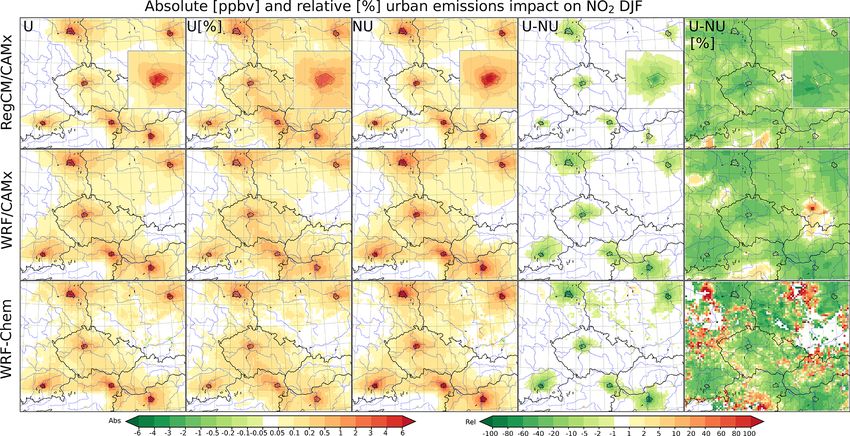
P. Huszar et al.: The regional impact of urban emissions                                                                    14313

al., 2020). Land use information adopted in model simula-                 i ∈ {URBAN, NOURBAN}.                                (2)
tions was derived from the high-resolution (100 m) CORINE
Land Cover (CLC) 2012 data (https://land.copernicus.eu/             The relative impact will be evaluated as
pan-european/corine-land-cover, last access: 24 Septem-
ber 2021) and the United States Geological Survey (USGS)                       Ci (all emissions) − Ci (zero urban emissions)
                                                                  UEIi,rel =
database for grid cells without CORINE information. An im-                                    Ci (all emissions)
portant difference between WRF and RegCM models is that                        × 100 %, i ∈ {URBAN, NOURBAN}                  (3)
the latter one, fractional land use, is considered, while in
WRF, each grid cell is designated the dominant land use.          for NO2 and PM2.5 , i.e., the relative contribution of urban
                                                                  emissions to the total concentration is provided. For O3 ,
2.2.1   Model simulations                                         UEIi,rel is calculated as

To fulfill the goal of the study, several simulations have been                Ci (all emissions) − Ci (zero urban emissions)
                                                                  UEIi,rel =
performed with and without including the effects of both the                             Ci (zero urban emissions)
urban canopy meteorological forcing and the chemical foot-                     × 100 %, i ∈ {URBAN, NOURBAN},                 (4)
print of the urban emissions (i.e., the UEI). Part of the sim-
ulations that are analyzed in this work had been already an-      i.e., this number gives the relative change in the concentra-
alyzed in Huszar et al. (2020b): these included experiments       tion after introducing urban emissions.
with all emissions considered but with or without consider-          The relative 1(UEI) presented throughout the article is
ing the UCMF. As the focus of this paper is to evaluate the       calculated as
impact of urban emissions, we extend these simulations with
those without the inclusion of such emissions (for selected                      UEIURBAN − UEINOURBAN
                                                                  1(UEI)rel =                          .                       (5)
cities). The complete list of simulations performed is in-                            UEINOURBAN
cluded in Table 1. The regional climate simulations included
                                                                  2.2.2   Emission processing
two experiments with the RegCM model, with (“URBAN”)
and without (“NOURBAN”) considering the urban canopy              For Europe, emissions provided by CAMS (Copernicus At-
meteorological effects (simulated by the CLMU urban mod-          mosphere Monitoring Service) version CAMS-REG-APv1.1
ule), and two experiments with the WRF-Chem model, again          inventory (regional–atmospheric pollutants; Granier et al.,
with and without considering urban canopies (simulated by         2019) for the year 2015 were used as anthropogenic emis-
the SLUCM module).                                                sions. For the Czech Republic, the high-resolution national
   The chemistry transport model simulations encompass            Register of Emissions and Air Pollution Sources (REZZO)
CAMx runs based on RegCM and WRF-Chem regional cli-               dataset issued by the Czech Hydrometeorological Institute
mate reconstructions and that corresponding to the chemical       (https://www.chmi.cz, last access: 24 September 2021) along
component of WRF-Chem. For each CTM, in total four sim-           with the ATEM traffic emissions dataset provided by ATEM
ulations are repeated. In two, the default emission data (i.e.,   (Ateliér ekologických modelů – Studio of ecological mod-
all emissions) are considered, while the inclusion of urban       els; https://www.atem.cz, last access: 24 September 2021)
effect is once included and then excluded. In the other two,      was used. These data offer activity-based (SNAP – Selected
urban emissions for selected cities were completely removed       Nomenclature for sources of Air Pollution) annual emission
(see Sect. 2.2.2), i.e., adopting the annihilation method (Bak-   sums of main pollutants, namely oxides of nitrogen (NOx ),
lanov et al., 2016). Finally, two additional simulations with     volatile organic compounds (VOCs), sulfur dioxide (SO2 ),
CAMx driven by RegCM meteorology were performed to an-            carbon monoxide (CO), PM2.5 and PM10 (particles with a
alyze the effect of the UCMF-induced changes in the vertical      diameter less than 2.5 and 10 µm). CAMS’ data are defined
eddy diffusion (Kv) and their contribution to the modeled ur-     on a Cartesian grid. On the other hand, the Czech REZZO
ban emission impact.                                              and ATEM datasets are defined as area, line (for road trans-
   This strategy of experimental design allows us to evaluate     portation) or point sources, while in the case of the first these
the UEI for both the URBAN and NOURBAN cases and an-              are usually irregular shapes that correspond to counties with
alyze their difference or, in other words, to investigate how     resolutions from a few hundred meters to 1–2 km depending
the emission impact is modulated by the UCMF. Thus, the           on the geometry of the particular shape, so they are appropri-
main focus is on the evaluation of                                ate for resolving urban emissions at 1 km domain resolution
                                                                  (in the case of Prague).
1UEI = UEIURBAN − UEINOURBAN ,                             (1)
                                                                     Data from the listed emissions inventories are prepro-
where the UEI for URBAN or NOURBAN cases is evaluated             cessed using the FUME (Flexible Universal Processor for
for a pollutant C as                                              Modeling Emissions) emission model (http://fume-ep.org/,
                                                                  last access: 24 September 2021; Benešová et al., 2018).
UEIi = Ci (all emissions) − Ci (zero urban emissions),            FUME is designed primarily for preparation of CTM-ready

https://doi.org/10.5194/acp-21-14309-2021                                        Atmos. Chem. Phys., 21, 14309–14332, 2021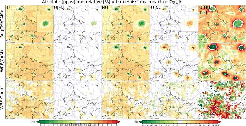
14314 P. Huszar et al.: The regional impact of urban emissions
Table 1. The list of model simulations performed: the first section contains the RCM simulations that cover the whole analyzed period
with the information of whether urban land surface was considered (second column). The second section lists the performed regional CTM
experiments – here the second column provides information on the driving meteorological data (not needed in the case of WRF-Chem).
Regional climate model (RCM) runs
Model Urbanizationa Resolution [km]
RegCM Yes 9/3/1b
RegCM No 9/3/1
WRF-Chem Yes 9
WRF-Chem No 9
Regional chemistry transport model (CTM) runs
Model Emission scenario Driving data Resolution [km]
CAMx All RegCM9U(/3U/1U) 9/3/1
CAMx No urban RegCM9U(/3U/1U) 9/3/1
CAMx All RegCM9NU(/3NU/1U) 9/3/1
CAMx No urban RegCM9NU(/3NU/1U) 9/3/1
WRF-Chem URBAN All –c 9
WRF-Chem URBAN No urban – 9
WRF-Chem NOURBAN All – 9
WRF-Chem NOURBAN No urban – 9
CAMx All WRF-Chem URBAN 9
CAMx No urban WRF-Chem URBAN 9
CAMx All WRF-Chem NOURBAN 9
CAMx No urban WRF-Chem NOURBAN 9
CAMx All RegCM9NKVd (/3NKV/1NKV) 9/3/1
CAMx No urban RegCM9NKV(/3NKV/1NKV) 9/3/1
a Information of whether urban land surface was considered. b Simulation performed in a nested way at 9, 3 and 1 km. c No driving
meteorological data needed as chemistry is online coupled to the parent meteorological model. d NKV – not considering the
urban-induced modifications of the vertical-eddy-diffusion coefficients.
emission files, including preprocessing the raw input files, public database (https://gadm.org, last access: 24 Septem-
the spatial redistribution of the data into the model grid, ber 2021) for the definition of administrative boundaries of
chemical speciation and time disaggregation of input emis- the cities selected in this study. For the second task, the
sions. Category-specific speciation factors (Passant, 2002) masking of inventory emissions based on the GADM shapes
and time disaggregation (van der Gon et al., 2011) are ap- corresponding to cities, we had to ensure correct partition
plied to derive hourly speciated emissions for CAMx and between the “city” and “non-city” portion of those shapes
WRF-Chem models. Biogenic emissions of hydrocarbons which spawn over the city boundaries. For this purpose, the
(BVOCs) for CAMx runs are calculated offline using the masking capability of FUME was used, which allows us to
MEGANv2.1 (Model of Emissions of Gases and Aerosols define an arbitrary mask for subsetting emissions either in-
from Nature version 2.1) emissions model (Guenther et al., side or outside of the mask. To demonstrate the resulting
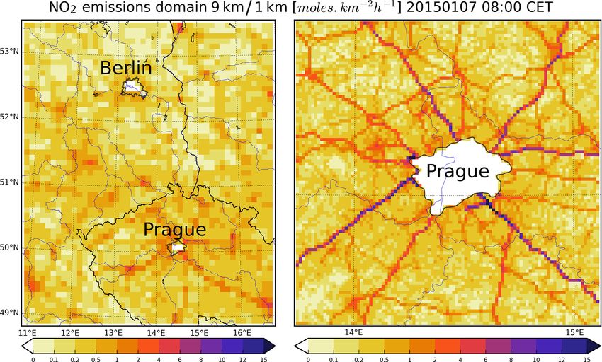
2012) based on RegCM and WRF meteorology. In the case masked emissions for the case of Berlin and Prague at 9 and
of WRF-Chem experiments, they are calculated online based 1 km resolution, we plotted in Fig. 2 the emissions of NO2 for
on the MEGAN approach. The necessary inputs for MEGAN a selected hour. It is seen that (correctly) only those grid cells
(plant functional types, emission factors and leaf-area-index that are entirely encompassed within the city have zero emis-
data) were derived based on Sindelarova et al. (2014). sions. Grid cells that have a part not in the city have non-zero
To isolate the emissions originating from urban areas from emissions. Cities considered are Prague, Berlin, Munich, Bu-
those from elsewhere, various approaches are possible: one dapest, Vienna and Warsaw, selected based on multiple crite-
can select the grid boxes (or other shapes) in the source in- ria: (a) city size should be such that at least a few grid cells in
ventories that lie inside the city’s limits or the same can be the 9 km domain cover the city, (b) cities are sufficiently far
applied for the already redistributed emission on the model from each other to eliminate inter-city influences (see Huszar
grid. Once either approach is selected, first the city bound- et al., 2016a), (c) the terrain of the city should have min-
aries have to be properly defined. For this purpose, we used imal variability to eliminate orographic effects (Ganbat et
the Database of Global Administrative Boundaries (GADM) al., 2015), and (d) cities should be distant from large water
Atmos. Chem. Phys., 21, 14309–14332, 2021 https://doi.org/10.5194/acp-21-14309-2021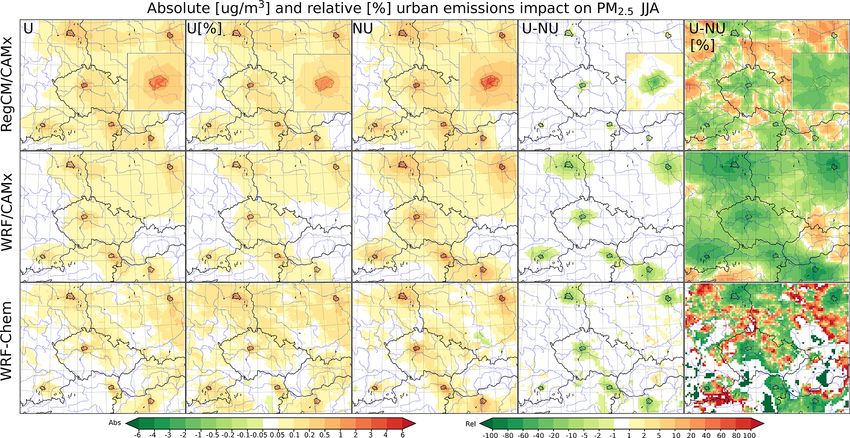
P. Huszar et al.: The regional impact of urban emissions                                                                       14315

Table 2. The list of cities, their population (in million), area (in   mated mainly during summer and is probably connected to
km2 ) and population density (in km−2 ) based on Eurostat (2021)       overestimation riming caused by increased graupel sedimen-
data.                                                                  tation in deep convective clouds. Furthermore, both mod-
                                                                       els show some overestimation of 10 m wind speeds and a
       City        Population     Area    Population density           reasonable reproduction of the maximum daily PBL heights
                    (million)    [km2 ]             [km−2 ]            with WRF performing better than the RegCM model which
       Berlin             3.7      891                  4150           slightly overestimates it, caused probably by the strong ver-
       Budapest           1.8      525                  3430           tical turbulent transport in the Holtslag scheme that RegCM
       Munich             1.5      310                  4840           uses.
       Prague             1.3      298                  4360              The simulated annual variation in monthly mean modeled
       Vienna             1.8      414                  4350           and measured air quality data is shown in Fig. 3, while for
       Warsaw             1.7      517                  3290           each city, the average of all available urban background sta-
                                                                       tions is used. NO2 is systematically underestimated in all
                                                                       models and all cities by about 10–20 µg m−3 , suggesting ei-
bodies and/or sea to eliminate non-symmetric land use ef-              ther low emission values or incorrect NO/NO2 speciation in
fects around the city (e.g., sea breeze effects; Ribeiro et al.,       the FUME emission model, supported also by the fact that
2018). We admit that the selection could follow a more ob-             the diurnal cycles usually are well captured with respect to
jective criteria like number of inhabitants or area; however,          their shape (only the systematic underestimation mentioned
we assumed (and our results showed) that the differences in            earlier persists). In the case of ozone (O3 ), it is strongly
results between cities are qualitatively very small, and the           overestimated (by up to 20–30 µg m−3 in all simulations, be-
choice of the list of cities from the region examined has thus a       ing the largest in the RegCM-driven one). In Huszar et al.
very small effect on the results. Additional information about         (2020b) it was shown that this is given mainly by a night-
cities including population, size and population density is in-        time positive bias reaching 40 µg m−3 which emerges from
cluded in Table 2. It shows that the cities are of very similar        inaccuracies in nighttime chemistry and deficiencies in cap-
size with populations between 1–2 million inhabitants with             turing nocturnal vertical eddy transport (Zanis et al., 2011).
Berlin as an exception of a larger city with a population of           Huszar et al. (2020b) also showed that high-resolution exper-
3.7 million. Most of the emitted polluting material from these         iments are more successful in capturing the day-to-day vari-
cities is in the form of CO and NO2 (Huszar et al., 2016a).            ation in NO2 values probably as a result of the higher reso-
Most of the cities emit primarily in the transport sector, while       lution of emission data and also due to better representation
residential heating and energy production are also important           of the terrain and hence the meteorological conditions. Fi-
(energy production being the primary source for Warsaw).               nally, PM2.5 is usually underestimated in models by around
                                                                       10 µg m−3 throughout the year with the smallest biases en-
                                                                       countered in the WRF-driven CAMx experiment. This nega-
3     Results                                                          tive bias was attributed in Huszar et al. (2020b) to underesti-
                                                                       mated nitrate aerosol formation and also to strongly underes-
3.1    Model validation                                                timated organic aerosol which is an important component of
                                                                       the urban PM2.5 burden. As for the influence of these model
Both the regional climate and chemistry transport model ex-            deficiencies on the results, the underestimation of NO2 and
periments presented here (those considering all emissions;             PM2.5 means that the UEI will be somewhat underestimated
see Table 1) were subject to validation in Huszar et al.               too in our models. In the case of ozone, which is usually over-
(2020b) based on European E-OBS (version 20.0e) mete-                  estimated except summer maximum values, it is expected
orological and AirBase air quality data (https://www.eea.              that the average impact of UEI (decreases, see below) will
europa.eu/data-and-maps/data/aqereporting-8, last access:              be slightly underestimated in the model.
24 September 2021). Here we summarize only the most rel-
evant conclusions for the validation of meteorological fields,
                                                                       3.2   The impact of urban emissions
while for the chemical validation, we provide the compari-
son of the annual cycle of the pollutants in focus for each
analyzed city. Regarding meteorology, it was shown that                In our analysis we will focus on the near-surface concentra-
each model performs reasonably within accepted range of                tions of NO2 , PM2.5 and O3 . First, the impact on seasonal –
biases and is comparable to other studies using very simi-             DJF (winter) and JJA (summer) – averages will be presented.
lar model configurations (Berg et al., 2013; Karlický et al.,          As different emissions and chemical regimes occur during
2017, 2018). In general, RegCM precipitation is well cap-              the day, the diurnal cycles are of interest too. Further, given
tured in all seasons, while the winter temperatures are some-          their high policy relevance, the impact on the extreme values
how larger than measured ones connected probably to re-                will be evaluated as well. Finally, we will look how the ver-
duced thermal cooling. For WRF, precipitation is overesti-             tical turbulent diffusion, as the most important component of

https://doi.org/10.5194/acp-21-14309-2021                                            Atmos. Chem. Phys., 21, 14309–14332, 2021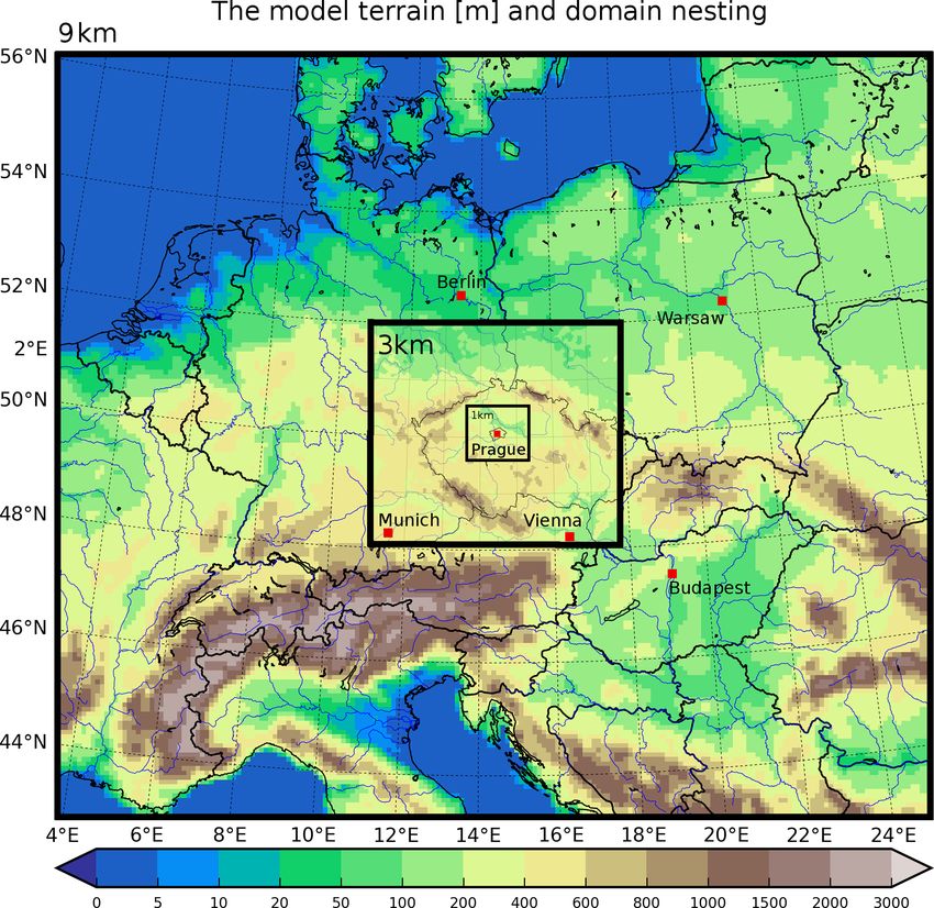
14316                                                                  P. Huszar et al.: The regional impact of urban emissions

Figure 2. Demonstration of the masked NO2 emissions for Prague and Berlin for the 9 and 1 km domains (in mol km−2 h−1 ) (only a part of
the domains is shown).

Figure 3. Comparison of the modeled average annual variation in monthly means with observations for the six selected cities and three
pollutants: NO2 , O3 and PM2.5 (in µg m−3 ). The black line means observations, and red, yellow and sky blue stand for RegCM/CAMx,
WRF-Chem and WRF/CAMx models.

UCMF, alone explains the modeled impact of (not) consider-            urban emissions to the total concentrations is in the second
ing the urban canopy meteorological effects.                          one. Higher values of the impact of up to 4–6 ppbv are seen
                                                                      for each analyzed city, and the similarities between models
3.2.1   Seasonal impact                                               are very large. This corresponds to the contribution of ur-
                                                                      ban emissions of around 40 %–60 % for urban centers. The
                                                                      impact quickly becomes small further from cities with in-
In Fig. 4 the winter UEI for NO2 is presented for the three
                                                                      creases up to 1 ppbv over rural areas corresponding to about
applied modeling systems: RegCM/CAMx (9 and 1 km hor-
                                                                      a 5 %–10 % contribution. The impact is not completely sym-
izontal resolution), WRF/CAMx and WRF-Chem (both with
                                                                      metric around cities owing to the prevailing wind directions.
only 9 km resolution). The first two columns shows the UEI
                                                                      If calculating the UEI on the 1 km domain (case of Prague), it
evaluated from the URBAN experiments, the absolute im-
                                                                      reveals some details of the emission structure of the city with
pact shown in the first one, while the relative contribution of

Atmos. Chem. Phys., 21, 14309–14332, 2021                                              https://doi.org/10.5194/acp-21-14309-2021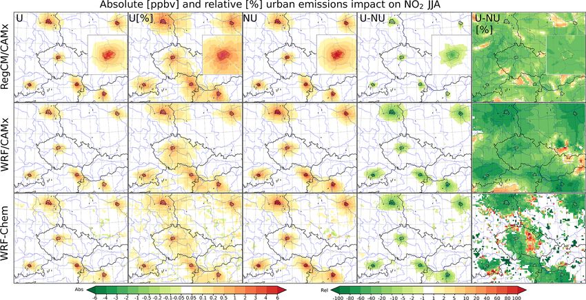
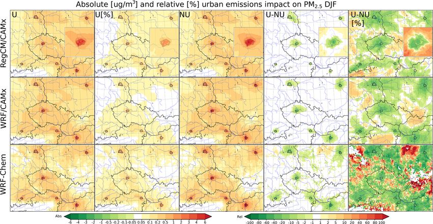
P. Huszar et al.: The regional impact of urban emissions                                                                   14317

a maximum impact of 6 ppbv that corresponds to a 60 %–             and −3 µg m−3 corresponding to about a 40 %–60 % smaller
80 % contribution and so providing a somehow larger rela-          impact in the URBAN case compared to NOURBAN one
tive impact for the city core if a higher resolution is applied.   for the city centers. The difference between the URBAN
The UEI impact evaluated from the NOURBAN is evidently             and NOURBAN UEI can be even positive, e.g., above ru-
larger (third and fourth columns), exceeding 6 ppbv for each       ral Poland or also seen around Prague in the 1 km resolution
analyzed city and model too. In other words, the impact            runs. This can be explained by the fact that UCMF causes
of city emissions is smaller if URBAN effects are consid-          stronger turbulent removal of the urban emissions, but this
ered, and this difference can reach 2–3 ppbv, especially in the    results in enhanced sedimentation further from cities leading
WRF-Chem experiments. The impact over areas surrounding            to higher emission footprint there (especially in the WRF-
cities is larger in the urbanized runs by about 0.1–0.2 ppbv,      Chem experiments).
quickly becoming zero further from cities where the UCMF              During JJA (Fig. 7), the PM2.5 urban-emission-induced
becomes negligible. In relative numbers, the decrease in UEI       concentration changes for both the URBAN and NOURBAN
modeled for the URBAN case is about 20 %–40 % and is               cases resemble the situation in DJF quantitatively, but they
seen for larger areas not limited to the analyzed cities. How-     are smaller, up to 2 µg m−3 in all models and cities. They are
ever, over areas where both the absolute city impact (UEI)         larger, reaching 4 µg m−3 in the high-resolution experiments
and the difference 1UEI is small, this relative decrease is a      for Prague where the concentrated character of sources is
result of the ratio of two very small numbers and should be        better resolved. In relative numbers, the contribution makes
regarded with caution. This holds for areas where the rela-        about 20 %–40 % (except the city core in Prague at high res-
tive change in 1UEI is positive, which means stronger urban        olution reaching 60 %). If the UCMF is considered, the UEI
emission impact for the URBAN compared to NOURBAN                  decreased by about 1–2 µg m−3 with the exception of Prague
case. This is, however, explainable by the fact that in the        in high resolution reaching a −3 µg m−3 decrease.
former case, the stronger urban turbulence removes pollu-             The impact of urban emissions on regional ozone (Fig. 8)
tants more effectively and the deposition occurs at larger dis-    follows a different pattern than for NO2 and PM2.5 . As a sec-
tances leading to concentration increase (see Huszar et al.,       ondary gas, its responses to increased emissions of its precur-
2020b); although these changes are very small in absolute          sors (NOx and NMVOC) depend not only on the magnitude
numbers, so the relative difference between the URBAN- and         of each precursor but also on their ratio. In the case of CAMx
NOURBAN-based UEI should be again treated with caution.            (either driven by RegCM or WRF meteorology), introducing
   For the case of JJA in Fig. 5, the results are qualitatively    urban emissions resulted in a clear O3 decrease above the se-
very similar to DJF. The absolute impact of urban emis-            lected urban areas reaching a −2 to −3 ppbv decrease as JJA
sions is somewhat smaller, usually reaching 4 ppbv and be-         average for the 9 km experiments while exceeding −4 ppbv
ing largest in the RegCM/CAMx model. The spatial extent of         for Prague at 1 km. In relative numbers, this represents a de-
the impact larger than 0.05 ppbv is also smaller than in DJF.      crease by up to 10 %–20 % (but usually between −5 % and
This is an expected consequence of in general lower sum-           −10 %) compared to the background concentrations (that do
mer emissions due to the missing domestic heating source           not consider urban emissions). The UEI over rural areas sur-
and also due to larger mixing into higher model levels allow-      rounding cities manifests itself as a slight increase in ozone
ing transport to distant areas. The relative contribution of ur-   by up to 0.5–1 ppbv (a few percentage points in relative num-
ban emissions to the final concentrations is also smaller than     bers). For the NOURBAN case, the decrease in O3 is stronger
in JJA. The UEI for the NOURBAN case leads again to a              for each city, usually exceeding −4 ppbv or even −6 ppbv
higher emission impact reaching 6 ppbv (slightly higher than       in the high-resolution runs for Prague. This means that the
in the winter case). The spatial extent is, however, smaller       UEI for ozone is weaker in the URBAN case by around 2–
than during DJF. This resulted in a different 1UEI pattern in      3 ppbv. For areas surrounding cities, where ozone increased
JJA: the spatial extent of the decrease for the URBAN case is      due to the urban emissions, the UEI difference between the
smaller; however, for urban cores, the decrease in the impact      URBAN and NOURBAN cases is positive too, meaning that
is larger compared to DJF. The relative change in the UEI is       the ozone increase due to UEI is larger in the URBAN case.
also larger during this season, often exceeding 60 %.              In relative numbers, the change in UEI due to the introduc-
   For PM2.5 , again, the general conclusions are similar to       tion of the UCMF is often larger than −60 % (stronger in
NO2 . The winter UEI (Fig. 6) reaches 4–6 µg m−3 for the           the WRF-driven CAMx runs). For city vicinities, the relative
analyzed cities and reaches 0.5 µg m−3 for rural areas. The        change in UEI reaches high values too, up to 100 % increase.
relative contribution of urban emissions to the PM2.5 con-            A different picture is gained if the UEI is evaluated for
centrations for the city centers and rural areas is about          ozone based on the WRF-Chem model. The addition of urban
20 %–40 % and 1 %–5 %, respectively. The UEI evaluated             emissions leads here to either no change or a little increase
for the NOURBAN case is again stronger, often exceed-              in the average summer ozone, indicating a different ozone
ing 6 µg m−3 ; the rural impact is, however, very similar to       isopleth pattern in the case of the RADM2 mechanism used
the URBAN case. The decrease in UEI due to the inclu-              in the mentioned model (for more details, see the Discus-
sion of urban effects (i.e., the UCMF) is usually between −2       sion). For most of the analyzed cities, the UEI means about

https://doi.org/10.5194/acp-21-14309-2021                                        Atmos. Chem. Phys., 21, 14309–14332, 2021
14318                                                                 P. Huszar et al.: The regional impact of urban emissions

Figure 4. The urban emission impact (UEI) of six selected cities (Berlin, Budapest, Munich, Prague, Vienna and Warsaw) on average DJF
near-surface NO2 concentrations from 2015 to 2016 for the three modeling systems used: CAMx driven by RegCM (first row), CAMx
driven by WRF-Chem meteorology (second row) and WRF-Chem (third row). Individual columns represent the UEI evaluated for the
URBAN experiments as absolute (UEIURBAN ; U; in ppbv) and relative impact (UEIURBAN,rel ; U[%]), the UEI impact for the non-urbanized
(NOURBAN) experiments (UEINOURBAN ; NU), the difference between the two (1UEI; U-NU), and the relative change in the impact
(1(UEI)rel ; in %). The corresponding results for Prague at 1 km resolution from the RegCM-driven CAMx experiments are plotted within
the 9 km figures in the upper row.

Figure 5. Same as Fig. 4 but for JJA.

Atmos. Chem. Phys., 21, 14309–14332, 2021                                            https://doi.org/10.5194/acp-21-14309-2021
P. Huszar et al.: The regional impact of urban emissions                                                              14319

Figure 6. Same as Fig. 4 but for PM2.5 (in µg m−3 ).

Figure 7. Same as Fig. 6 but for JJA.

a 0.5 ppbv increase in ozone, while for Berlin, it is rather    a rather complicated pattern; however, it is a result of the
characterized by a slight decrease (around −0.1 ppbv). These    ratio of very small, almost insignificant changes. What one
slight changes constitute a very small relative change on the   can state for certainty is that in the WRF-Chem model, urban
order of up to 5 %. The UEI is slightly smaller in magni-       emissions lead to a rather slight ozone increase above cities
tude in the NOURBAN case. In relative numbers one obtains

https://doi.org/10.5194/acp-21-14309-2021                                     Atmos. Chem. Phys., 21, 14309–14332, 2021
14320                                                            P. Huszar et al.: The regional impact of urban emissions

Figure 8. Same as Fig. 5 but for O3 .

which is stronger in the URBAN case than in the NOURBAN          ing nighttime and reaches its maximum during early evening
one.                                                             hours. In RegCM-driven CAMx the maximum reaches −3
                                                                 to −4 ppbv for DJF and JJA, respectively, while a much
3.2.2   Impact on diurnal cycles                                 stronger decrease is modeled with WRF meteorology reach-
                                                                 ing −12 ppbv. This is a much greater change in UEI (due
As the UCMF has a different magnitude throughout the day         to the UCMF) than seen for the seasonal means in Figs. 4
(e.g., the urban warming or heat island has a clear peak dur-    and 5. A second, smaller peak during morning hours is also
ing early night hours, while the urban boundary layer is         exhibited by each model that reaches values between −1 to
thickest during the day), one might expect that the differ-      −4 ppbv.
ent impacts of urban emissions between the URBAN and                A qualitatively very similar result is obtained for PM2.5
NOURBAN cases will have a specific diurnal cycle too. We         (Fig. 10). Again, the three models provide comparable re-
therefore calculated the average seasonal diurnal cycles of      sults. The UEI impacts for both the NOURBAN and UR-
concentrations from the analyzed urban centers (averaged         BAN cases follow strongly the typical pattern for the PM2.5
over all city).                                                  emissions exhibiting two peaks during rush hours. It is clear
   Figure 9 shows the DJF and JJA average diurnal cycles for     that the UEIs for the URBAN case are much lower reach-
surface NO2 concentrations from individual simulations and       ing 4–6 and 2–3 ppbv as peaks in DJF and JJA, respectively,
their differences (i.e., the UEIs and the 1UEIs). In general,    while the difference with respect to the NOURBAN UEI case
the three models perform in a very similar manner. The UEI       varies during the day. Its exact diurnal pattern is shown by the
impacts for both the NOURBAN (blue) and URBAN (or-               green line which, again, has a very clear pattern in both sea-
ange) cases follow strongly the typical pattern for the NOx      sons and all models. In absolute sense it is almost zero dur-
emissions exhibiting two peaks during morning and after-         ing nighttime and reaches its maximum during early evening
noon rush hours (the weekends have a somewhat weaker pat-        hours. In RegCM-driven CAMx the peak reaches −1.4 and
tern, but weekdays dominate the average). It is clear that the   −1.2 µg m−3 for DJF and JJA, respectively, while a much
UEI for URBAN case (dashed orange) is much lower, reach-         stronger decrease is modeled with WRF meteorology reach-
ing 10–15 and 5–10 ppbv as peaks in DJF and JJA, respec-         ing −5 µg m−3 in DJF (−3.5 µg m−3 during JJA). Similarly
tively, while the difference with respect to the NOURBAN-        to NO2 , this is a much greater change in UEI (due to the
based UEI (dashed blue) varies during the day. Its exact di-     UCMF) than seen for the seasonal means in Figs. 6 and 7.
urnal pattern is shown by the green line which has a very        A second, usually much smaller peak during morning hours
clear pattern in both seasons and all models (belongs to
right vertical axis). In absolute sense it is almost zero dur-

Atmos. Chem. Phys., 21, 14309–14332, 2021                                        https://doi.org/10.5194/acp-21-14309-2021
P. Huszar et al.: The regional impact of urban emissions 14321
is also exhibited by each model that reaches values between reaches 8 µg m−3 in each model (especially for Prague, Bu-
−1 to −2 µg m−3 . dapest and Warsaw). This is again higher than the impact on
In the case of ozone (Fig. 11), for the CAMx experiments, averages (up to 6 µg m−3 ) and points to the increased role
the UEI shows a strong correlation with the absolute values of urban emissions during extreme PM pollution events. Our
(dashed vs. solid lines) meaning that when urban ozone val- results also suggest a large impact over rural areas reaching
ues are lowest, also the UEI for O3 shows its maximum (in 1–2 µg m−3 , indicating potential for urban emissions to en-
absolute sense). The maximum impact occurs during morn- hance rural concentrations too. The decrease in the UEI of
ing and early evening hours, reaching −12 and −10 ppbv extreme values of PM2.5 if the UCMF is considered can be
for DJF for the NOURBAN and URBAN cases, respectively, as large as −4 to −6 µg m−3 . Again, this is a stronger de-
and reaching minimum values during noon and night. Dur- crease compared to the values obtained for the DJF and JJA
ing JJA, the UEI reaches −10 and −8 ppbv for the NOUR- averages (Figs. 6–7).
BAN and URBAN cases, while the UEI for the URBAN case In the case of ozone (Fig. 14), somehow different be-
is smaller in the WRF-driven CAMx experiment (reaching havior is modeled for CAMx and for WRF-Chem (simi-
−5 ppbv). In conclusion, in CAMx driven either by RegCM larly to the impact on seasonal averages), but differences are
or WRF, the UEI is negative during the whole day. in the case encountered between cities too. The UEI for the 95th per-
of WRF-Chem, the impact is expectedly negative throughout centile of the daily maximum 8 h O3 is usually negative over
the whole day in DJF, but for summer, it becomes positive cities, reaching −4 ppbv over city cores – this is the case of
during daytime, reaching 1.5 ppbv (the URBAN case being RegCM/CAMx and partly in WRF/CAMx too (for Berlin,
slightly higher). During night, the UEI reaches negative val- Warsaw, Prague and Budapest) with smaller decrease up to
ues of up to −1 ppbv for the NOURBAN case and −0.2 ppbv −1 ppbv. These are smaller decreases that those seen for av-
for the URBAN one. The 1UEI (green line) is rather positive erage JJA ozone in Fig. 8. On the other hand, for cities like
in each model and season showing a clear maximum during Budapest and Berlin in WRF/CAMx experiments and for all
late afternoon and evening hours, which reaches a few parts cities in WRF-Chem, the UEI for the 95th percentile ozone
per billion volume in DJF (0.5 in WRF-Chem), while in JJA values is positive with increases up to 2–4 ppbv in WRF-
the maximum can be as high as 10 ppbv. This indicates that Chem. For areas surrounding cities, further from the origin
the urban emission impact for ozone is smaller in absolute of the emissions, there is a clear increase in ozone reach-
sense if the model predicts its decrease due to UEI (CAMx), ing 1 ppbv over large areas. This indicates that during ex-
while it is higher if the model predicts an increase (WRF- treme ozone periods, urban emissions push the balance be-
Chem). tween the ozone production and reduction towards produc-
tion leading to smaller reductions for some cities and models
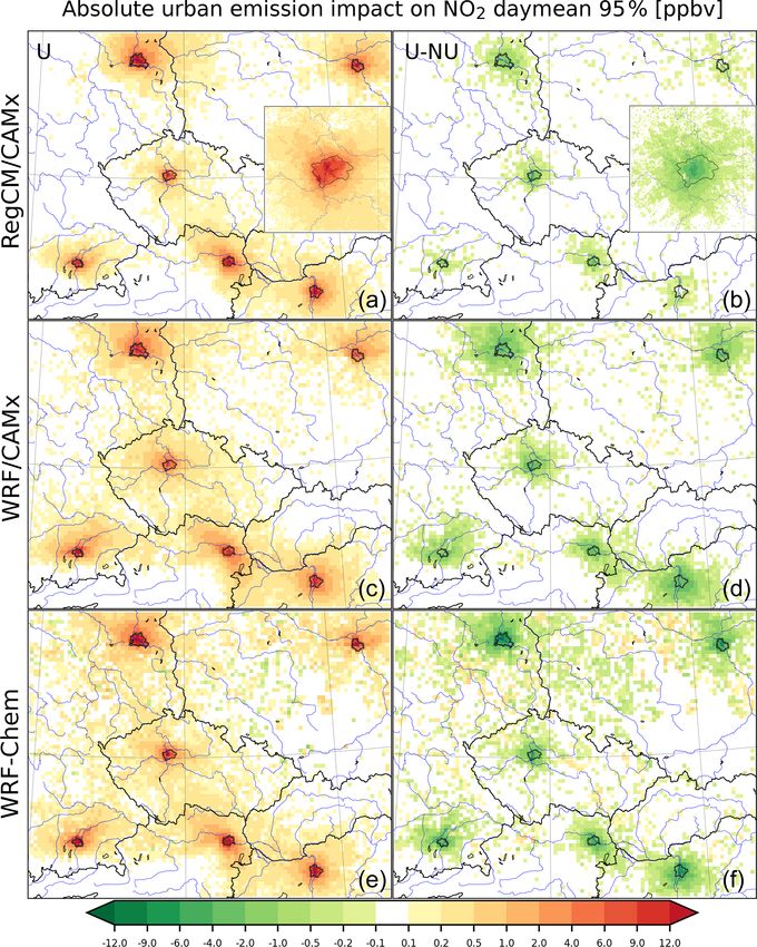
3.2.3 Impact on extreme values and stronger increase for other cities and models. The change
between the URBAN and NOURBAN cases is positive for
Huszar et al. (2020b) showed that the urban canopy mete- RegCM/CAMx similarly to the impact on averages, mean-
orological forcing has a stronger effect on extreme air pol- ing that the reduction of extreme ozone is smaller when the
lution (95th percentile of NO2 , PM2.5 and O3 ) compared to UCMF is considered, but this modification is smaller than
the average one. This motivates us to look also at the UEI that seen for average values. For other models, the modu-
for such situations. We therefore plotted the UEI on the 95th lation of UEI between URBAN and NOURBAN is rather
percentile values of the daily means of the analyzed pollu- small and can be negative or positive with the preference of
tants and were interested also in the associated differences negative change, i.e., enhancement of the UEI in the case of
between the UEI evaluated for the NOURBAN and URBAN the WRF-Chem model. This means that if extreme ozone re-
cases (i.e., 1UEI). In Fig. 12 we see that the UEI for the sponds to urban emissions with an increase, the increase is
95th percentiles of NO2 is much higher compared to the im- smaller if UCMF is considered. On the other hand, if ozone
pact on the average one and reaches 9–12 ppbv, especially in responds with a decrease, then this decrease is smaller in ab-
the WRF-Chem model (left column). It can also be seen that solute values when not considering UCMF.
it reaches 4–6 ppbv (i.e., the values seen for the averages) at
distances roughly twice the city size, indicating the crucial 3.2.4 The role of vertical turbulence
role urban emissions play in extreme air pollution events at
regional scales. Regarding the modulation of the emission As seen in previous sections, the urban emission impact is
impact by the UCMF (the right column), it is seen that it is significantly perturbed if the urban canopy meteorological
also much higher compared to the difference in the case of forcing is considered in its model estimation, and it is usually
averages and can reach −6 ppbv. This means that the UEI on overestimated if UCMF is disregarded. Many previous stud-
extreme air pollution is even more strongly reduced by the ies showed that the most important component of the UCMF
urban effects that the averages seen in Figs. 4–5. influencing the urban air pollution is the vertical eddy diffu-
In the case of PM2.5 in Fig. 13, the UEI for the 95th per- sion (e.g., Zhu et al., 2015; Huszar et al., 2020a). To evalu-
centiles is again higher than calculated for the averages and ate its role and contribution to the changes in UEI between
https://doi.org/10.5194/acp-21-14309-2021 Atmos. Chem. Phys., 21, 14309–14332, 202114322 P. Huszar et al.: The regional impact of urban emissions Figure 9. The average diurnal cycle of the absolute urban NO2 concentrations and their difference between different simulations for DJF (a– c) and JJA (d–f) and for the three models applied as columns: CAMx driven by RegCM, CAMx driven by WRF and WRF-Chem. Blue and orange lines denote the NOURBAN and URBAN cases, respectively. Solid lines stand for the reference values with 100 % urban emissions, dotted lines for the 0 % urban emission runs and dashed ones for the UEI evaluated for both the NOURBAN and URBAN cases. These correspond to the left vertical axis. Finally, the green line denotes the 1UEI (right vertical axis), i.e., the modification of the urban emission impact due to the inclusion of the urban effects (the UCMF). Units in parts per billion volume (ppbv). Figure 10. Same as Fig. 9 but for PM2.5 (in µg m−3 ). Atmos. Chem. Phys., 21, 14309–14332, 2021 https://doi.org/10.5194/acp-21-14309-2021
You can also read