Meteorology-driven variability of air pollution (PM1) revealed with explainable machine learning
←
→
Page content transcription
If your browser does not render page correctly, please read the page content below
Atmos. Chem. Phys., 21, 3919–3948, 2021
https://doi.org/10.5194/acp-21-3919-2021
© Author(s) 2021. This work is distributed under
the Creative Commons Attribution 4.0 License.

Meteorology-driven variability of air pollution (PM1)
revealed with explainable machine learning
Roland Stirnberg1,2 , Jan Cermak1,2 , Simone Kotthaus3 , Martial Haeffelin3 , Hendrik Andersen1,2 , Julia Fuchs1,2 ,
Miae Kim1,2 , Jean-Eudes Petit4 , and Olivier Favez5
1 Institute of Meteorology and Climate Research, Karlsruhe Institute of Technology (KIT), Karlsruhe, Germany
2 Institute of Photogrammetry and Remote Sensing, Karlsruhe Institute of Technology (KIT), Karlsruhe, Germany
3 Institut Pierre Simon Laplace, École Polytechnique, CNRS, Institut Polytechnique de Paris, Palaiseau, France
4 Laboratoire des Sciences du Climat et de l’Environnement, CEA/Orme des Merisiers, Gif sur Yvette, France
5 Institut National de l’Environnement Industriel et des Risques, Parc Technologique ALATA, Verneuil en Halatte, France

Correspondence: Roland Stirnberg (roland.stirnberg@kit.edu)

Received: 13 May 2020 – Discussion started: 27 July 2020
Revised: 4 February 2021 – Accepted: 9 February 2021 – Published: 17 March 2021

Abstract. Air pollution, in particular high concentrations of      related to residential heating, amounting to a contribution
particulate matter smaller than 1 µm in diameter (PM1 ), con-      to predicted PM1 concentrations of as much as ∼ 9 µg/m3 .
tinues to be a major health problem, and meteorology is            Northeasterly winds are found to contribute ∼ 5 µg/m3 to
known to substantially influence atmospheric PM concentra-         predicted PM1 concentrations (combined effects of u- and
tions. However, the scientific understanding of the ways in        v-wind components), by advecting particles from source re-
which complex interactions of meteorological factors lead to       gions, e.g. central Europe or the Paris region. Meteorolog-
high-pollution episodes is inconclusive. In this study, a novel,   ical drivers of unusually high PM1 concentrations in sum-
data-driven approach based on empirical relationships is used      mer are temperatures above ∼ 25 ◦ C (contributions of up to
to characterize and better understand the meteorology-driven       ∼ 2.5 µg/m3 ), dry spells of several days (maximum contribu-
component of PM1 variability. A tree-based machine learn-          tions of ∼ 1.5 µg/m3 ), and wind speeds below ∼ 2 m/s (max-
ing model is set up to reproduce concentrations of speciated       imum contributions of ∼ 3 µg/m3 ), which cause a lack of dis-
PM1 at a suburban site southwest of Paris, France, using me-       persion. High-resolution case studies are conducted showing
teorological variables as input features. The model is able        a large variability of processes that can lead to high-pollution
to capture the majority of occurring variance of mean af-          episodes. The identification of these meteorological condi-
ternoon total PM1 concentrations (coefficient of determina-        tions that increase air pollution could help policy makers to
tion (R 2 ) of 0.58), with model performance depending on          adapt policy measures, issue warnings to the public, or assess
the individual PM1 species predicted. Based on the mod-            the effectiveness of air pollution measures.
els, an isolation and quantification of individual, season-
specific meteorological influences for process understand-
ing at the measurement site is achieved using SHapley Ad-
ditive exPlanation (SHAP) regression values. Model results         1   Introduction
suggest that winter pollution episodes are often driven by
a combination of shallow mixed layer heights (MLHs), low           Air pollution has serious implications on human well-being,
temperatures, low wind speeds, or inflow from northeastern         including deleterious effects on the cardiovascular system
wind directions. Contributions of MLHs to the winter pol-          and the lungs (Hennig et al., 2018; Lelieveld et al., 2019)
lution episodes are quantified to be on average ∼ 5 µg/m3          and an increased number of asthma seizures (Hughes et al.,
for MLHs below < 500 m a.g.l. Temperatures below freez-            2018). This includes particles smaller than 1 µm in diame-
ing initiate formation processes and increase local emissions      ter (PM1 ), which are associated with fits of coughing (Yang
                                                                   et al., 2018) and an increase in emergency hospital visits

Published by Copernicus Publications on behalf of the European Geosciences Union.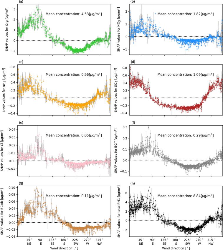
3920                                                        R. Stirnberg et al.: Meteorology-driven variability of air pollution

(Chen et al., 2017). The adverse health effect lead to an in-        2014; Petit et al., 2015, 2017; Dupont et al., 2016; Srivas-
crease in mortality of people exposed to high particle con-          tava et al., 2018). Results indicate that the Paris metropoli-
centrations (Samoli et al., 2008, 2013; Lelieveld et al., 2015).     tan region is often affected by mid-range to long-range
People living in urban areas are particularly affected by poor       transport of pollutants, as due to the city’s flat orogra-
air quality, and with increasing urbanization their number is        phy, an efficient horizontal exchange of air masses is fre-
projected to grow (Baklanov et al., 2016; Li et al., 2019).          quent (Bressi et al., 2013; Petit et al., 2015). High-pollution
These developments have motivated several countermeasures            events commonly occur in late autumn, winter, and early
to improve air quality. Proposed efforts to reduce anthro-           spring. Often, these episodes are characterized by stagnant
pogenic particle emissions include partial traffic bans (Su          atmospheric conditions and a combination of local contri-
et al., 2015; Dey et al., 2018) and the reduction of solid fuel      butions, e.g. traffic emissions, residential emissions, or re-
use for domestic heating (Chafe et al., 2014). Although emis-        gionally transported particles, such as ammonium nitrates
sions play an important role for PM concentrations in the            from manure spreading or sulfates from point sources (Pe-
atmosphere, meteorological conditions related to large-scale         tetin et al., 2014; Petit et al., 2014, 2015; Srivastava et al.,
circulation patterns as well as local-scale boundary layer           2018). High-pressure conditions with air masses originat-
processes and interactions with the land surface are major           ing from continental Europe (Belgium, Netherlands, west-
drivers of PM variability as well (Cermak and Knutti, 2009;          ern Germany) are generally associated with an increase in
Bressi et al., 2013; Megaritis et al., 2014; Dupont et al., 2016;    particle concentrations, especially of secondary inorganic
Petäjä et al., 2016; Yang et al., 2016; Li et al., 2017). Wind       aerosols (SIAs, Bressi et al., 2013; Srivastava et al., 2018).
speed and direction generally have a strong influence on air         The regional contribution has been found to be approxi-
quality as they determine the advection of pollutants (Petetin       mately 70 % for background concentrations in Paris of par-
et al., 2014; Petit et al., 2015; Srivastava et al., 2018). Lim-     ticles with a diameter smaller 2.5 µm (Petetin et al., 2014).
iting the vertical exchange of air masses, the mixed layer           Hence the variability between high-pollution episodes in
height (MLH) governs the volume of air in which particles            terms of timing, sources, and meteorological boundary con-
are typically dispersed. Although some authors indicate that         ditions is considerable (Petit et al., 2017). Previous ap-
mixed layer height cannot be related directly to concentra-          proaches to determine meteorological drivers of air pollution
tions of pollutants and that other meteorological parameters         included, for example, the use of chemical transport mod-
and local sources need to be considered (Geiß et al., 2017),         els (CTMs), which, however, require comprehensive knowl-
a lower MLH can increase PM concentrations as particles              edge on emission sources and secondary particle forma-
are not mixed into higher atmospheric levels and accumulate          tion pathways and are associated with considerable uncer-
near the ground (Gupta and Christopher, 2009; Schäfer et al.,        tainties (Sciare et al., 2010; Petetin et al., 2014; Kiesewet-
2012; Stirnberg et al., 2020).                                       ter et al., 2015). Further methods rely on data exploration,
    Higher MLHs in combination with high wind speeds in-             e.g. the statistical analysis of time series (Dupont et al.,
crease atmospheric ventilation processes, thus decreasing            2016), which can be coupled with positive matrix factoriza-
near-surface particle concentrations (Sujatha et al., 2016;          tion (PMF, Paatero and Tapper, 1994) to derive PM sources
Wang et al., 2018). Air temperature can influence PM con-            (Petit et al., 2014; Srivastava et al., 2018). To take into ac-
centrations in multiple ways, e.g. by modifying the emission         count the interconnected nature of PM drivers, multivariate
of secondary PM precursors such as volatile organic com-             statistical approaches such as principal component analysis
pounds (VOCs) during summer (Fowler et al., 2009; Megari-            (PCA) have been applied (Chen et al., 2014; Leung et al.,
tis et al., 2013; Churkina et al., 2017), and by condensat-          2017). In recent years, machine learning techniques have
ing high saturation vapour pressure compounds such as ni-            been increasingly used to expand the analysis of PM concen-
tric acid and sulfuric acid (Hueglin et al., 2005; Pay et al.,       trations with respect to meteorology, allowing general pat-
2012; Bressi et al., 2013; Megaritis et al., 2014). The wet re-      terns to be retraced (Hu et al., 2017; Grange et al., 2018).
moval of particles by precipitation is known to be an efficient      Here, the multivariate and highly interconnected nature of
atmospheric aerosol sink (Radke et al., 1980; Bressi et al.,         meteorology-dependent atmospheric processes influencing
2013), while moisture in the atmosphere can stimulate sec-           local PM1 concentrations at a suburban site southwest of
ondary particle formation processes (Ervens et al., 2011). Al-       Paris is analysed in a data-driven way. Therefore, a state-of-
though all these atmospheric conditions and processes have           the-art explainable machine learning model is set up to repro-
been identified as drivers of local air quality, it is usually a     duce the variability of PM1 concentrations, thereby capturing
complex combination of meteorological and chemical pro-              empirical relationships between PM1 concentrations and me-
cesses that lead to the formation of high-pollution events (Pe-      teorological parameters. The goal is to separate and quantify
tit et al., 2015; Dupont et al., 2016; Stirnberg et al., 2020).      influences of the meteorological variables on PM1 concen-
    The metropolitan area of Paris is one of the most densely        trations to advance the process understanding of the com-
populated and industrialized areas in Europe. Thus, air qual-        plex mechanisms that govern pollution concentrations at the
ity is a recurring issue and has been at the focus of many           measurement site. Localized (i.e. situation-based) and indi-
studies in recent years (Bressi et al., 2014; Petetin et al.,        vidualized attributions of feature contributions are performed

Atmos. Chem. Phys., 21, 3919–3948, 2021                                                https://doi.org/10.5194/acp-21-3919-2021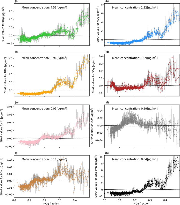
R. Stirnberg et al.: Meteorology-driven variability of air pollution 3921
using SHapley Additive exPlanation regression (SHAP) val-
ues (Lundberg and Lee, 2017; Lundberg et al., 2019, 2020),
allowing the meteorology-dependent processes driving PM
concentrations at high temporal resolution to be inferred.
Typical situations that lead to high PM1 concentrations are
identified, serving as a decision support to policymakers to
issue preventative warnings to the public if these situations
are to be expected. In addition, by directly accounting for me-
teorological effects on PM1 concentrations, such a machine-
learning-based framework could help in assessing the effec-
tiveness of measures towards better air quality. Furthermore,
the proposed ML framework can be viewed as a first step to-
wards a data-driven, prognostic tool in operational air quality
forecasting, complementary to CTM approaches.
2 Data sets
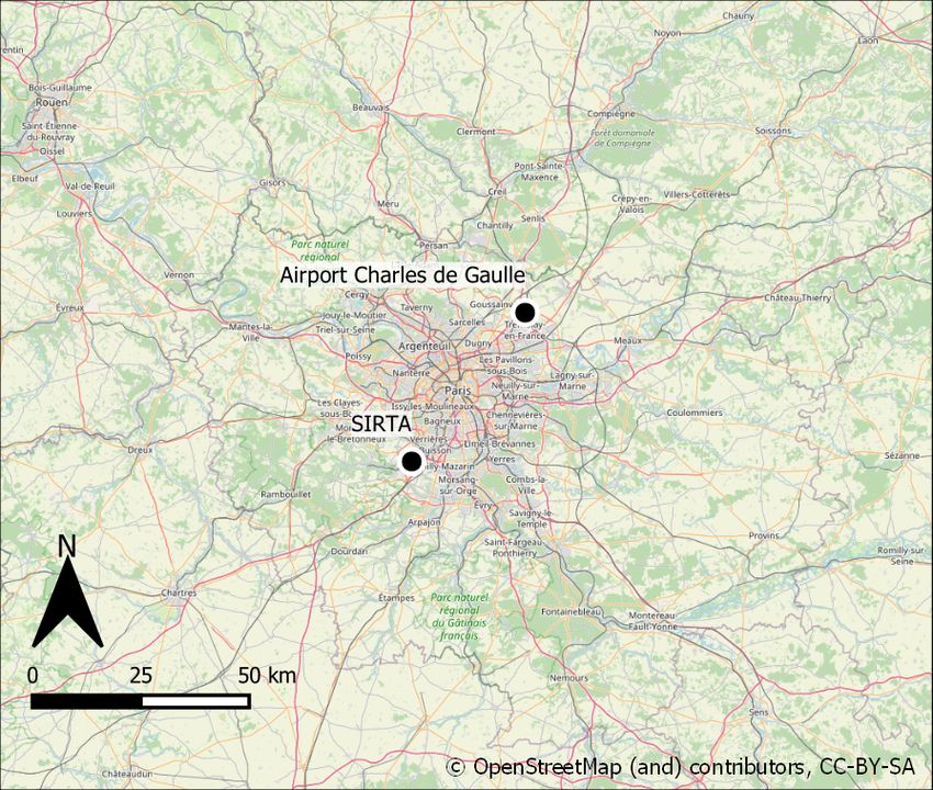
Seven years (2012–2018) of meteorological and air quality Figure 1. Location of the SIRTA supersite southwest of Paris.
data from the Site Instrumental de Recherche par Télédétec- © OpenStreetMap contributors 2020. Distributed under a Creative
tion Atmosphérique (SIRTA; Haeffelin et al., 2005) supersite Commons BY-SA License.
are the basis of this study. The SIRTA Atmospheric Observa-
tory is located about 25 km southwest of Paris (48.713◦ N
and 2.208◦ E; Fig. 1). This study focuses on day-to-day vari- in Petit et al. (2014). Using the multispectral information, a
ations of total and speciated PM1 , a highly health-relevant differentiation into fossil-fuel-based BC (BCff) and BC from
fraction of PM including small particles that can penetrate wood burning (BCwb) is achieved (Sciare et al., 2010; Healy
deep into the lungs (Yang et al., 2018; Chen et al., 2017). To et al., 2012; Petit et al., 2014; Zhang et al., 2019). Here, the
separate diurnal effects, e.g. the development of the bound- sum of all measured species is assumed to represent the to-
ary layer during morning hours (Petit et al., 2014; Dupont tal PM1 content (see Petit et al., 2014, 2015). The consis-
et al., 2016; Kotthaus and Grimmond, 2018a), from day- tency of ACSM and Aethalometer measurements is checked
to-day variations of PM1 , mean concentrations of total and by comparing the sum of all monitored species with measure-
speciated PM1 for the afternoon period 12:00–15:00 UTC ments of a nearby Tapered Element Oscillating Microbal-
are considered, when the boundary layer is fully developed. ance equipped with a Filter Dynamic Measurement System
In Sect. 2.1 and 2.2, the PM1 and meteorological data and (TEOM-FDMS). PM1 measurements are representative of
preprocessing steps before setting up the machine learning suburban background pollution levels of the region of Paris
model are described. The applied machine learning model (Petit et al., 2015). As an additional input to the machine
and data analysis techniques are presented in Sect. 3.1 and learning model, the average fraction of NO− 3 of the previ-
3.2. ous day is added (NO3_frac). Pollution events dominated by
NO− 3 are often linked to regional-scale events, which depend
2.1 Submicron particle measurements on anthropogenically influenced processes in the source re-
gions of NO− 3 precursors (Petit et al., 2017). This is approx-
Aerosol chemical speciation monitor (ACSM; Ng et al., imated by the inclusion of the average fraction of NO− 3 of
2011) measurements are conducted at SIRTA in the frame- the previous day, assuming that a high fraction of NO− 3 indi-
work of the ACTRIS project. The ACSM provides contin- cates the occurrence of such an anthropogenically influenced
uous and near-real-time measurements of the major chem- regime.
ical composition of non-refractory submicron aerosols, i.e.
2−
organics (Org), ammonium (NH+ 4 ), sulfate (SO4 ), nitrate 2.2 Meteorological data
− −
(NO3 ), and chloride (Cl ). A detailed description of its func-
tionality can be found in Ng et al. (2011). The data pro- Following the objective of this study, a set of meteorological
cessing and validation protocol can be found in Petit et al. variables is chosen as inputs for the ML model that either in-
(2015) and Zhang et al. (2019). In addition, black carbon fluence PM concentrations directly via dilution (MLH, wind
(BC) has been monitored by a seven-wavelength Magee Sci- speed (ws), and wet scavenging of particles (precipitation))
entific Aethalometer AE31 from 2011 to mid-2013, and a and particle transport (wind direction as u, v components, air
dual-spot AE33 (Drinovec et al., 2015) from mid-2013 on- pressure, AirPres), as a proxy for emissions (e.g. from resi-
wards. The consistency of both instruments has been checked dential heating: temperature at a height of 2 m (T )), and as a
https://doi.org/10.5194/acp-21-3919-2021 Atmos. Chem. Phys., 21, 3919–3948, 2021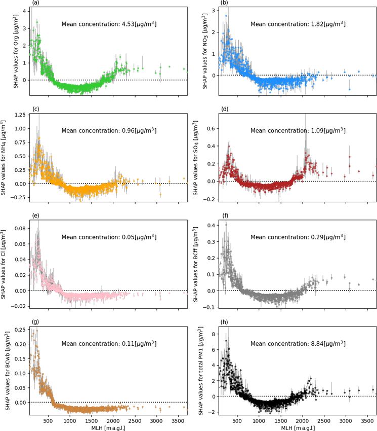
3922                                                      R. Stirnberg et al.: Meteorology-driven variability of air pollution

proxy for transformation processes (total incoming solar ra-       ing gradient descent (Friedman, 2002). This is an advantage
diation (TISR), relative humidity (RH), T ). Data are taken        of GBRT over standard ensemble tree methods (e.g. random
from the quality-controlled and 1 h averaged re-analysed ob-       forests (RF); Just et al., 2018) as trees are built systemat-
servation (ReObs) data set. Further information on the instru-     ically and fewer iterations are required (Elith et al., 2008).
mentation used for the acquisition of these variables is pro-      Characteristics of the meteorological training data set with
vided in Chiriaco et al. (2018). MLH is derived from auto-         respect to observed total and speciated PM1 concentrations
matic lidar and ceilometer (ALC) measurements of a Vaisala         are conveyed to the statistical model. The learned relation-
CL31 ceilometer using the CABAM algorithm (Character-              ships are then used for model interpretation and to produce
ising the Atmospheric Boundary layer based on ALC Mea-             estimates of PM1 based on unseen meteorological data to test
surements; Kotthaus and Grimmond, 2018a, b). Due to an             the model. The architecture of the statistical model is de-
instrument failure, during the period July to mid-November         termined by the hyperparameters, e.g. the number of trees,
2016, SIRTA ALC measurements had to be replaced with               the maximum depth of each tree (i.e. the number of split
measurements conducted at the Paris Charles de Gaulle Air-         nodes on each tree), and the learning rate (i.e. the magni-
port, located northeast of Paris. A comparison of measured         tude of the contribution of each tree to the model outcome,
MLHs at SIRTA and Charles de Gaulle Airport for the avail-         which is basically the step size of the gradient descent). The
able measurements in 2016 (Appendix A) shows generally             hyperparameters are tuned by executing a grid search, sys-
good agreement, which is why only minor uncertainties are          tematically testing previously defined hyperparameter com-
expected due to the replacement.                                   binations and determining the best combination via a three-
   Meteorological factors are chosen as input features for         fold cross-validation. Note that PM1 data are not uniformly
the statistical model based on findings of previous stud-          distributed; i.e. there are more data available for mid-range
ies (see Sect. 1). Meteorological observations are converted       PM1 concentrations. To avoid the model primarily optimiz-
to suitable input information for the statistical model (see       ing its predictions on these values, a least-squares loss func-
Sect. 3.1). Wind speed (ws) is derived from the ReObs u and        tion was chosen. This loss function is more sensitive to
v components [m/s], and the maximum wind speed of the af-          higher PM1 values (i.e. outliers of the PM1 data distribu-
ternoon period (12:00–15:00 UTC) is included in the model.         tion), as it strongly penalizes high absolute differences be-
U and v wind components are then normalized to values              tween predictions and observations. Accordingly, the model
between 0 and 1, thus only depicting the direction informa-        is adjusted to reproduce higher concentrations as well.
tion. To reduce the impact of short-term fluctuation in wind       For each PM species, a specific GBRT model is set up and
direction, the 3 d running mean is calculated based on the         used for the analysis of meteorological influences on individ-
normalized u and v wind components (umean and vmean).              ual PM1 species (see Sect. 4.2). Additionally, a quasi-total
Hours since the last precipitation event (Tprec) are counted       PM1 model is used to reproduce the sum of all species at
and used as input to capture the particle accumulation effect      once, which is used for an analysis of meteorological drivers
between precipitation events (Rost et al., 2009; Petit et al.,     of high-pollution events (see Sect. 4.3 and 4.4). Train and
2017).                                                             test data sets to evaluate each model are created by randomly
                                                                   splitting the full data set. These splits, however, are the same
                                                                   for the species models and the full PM1 model to ensure
3     Methods                                                      comparability between the models. Three-quarters of the data
                                                                   are used for training and hyperparameter tuning with cross-
3.1    Machine learning model: technique and application           validation (n = 1086), and one-quarter for testing (n = 363).
                                                                   In addition, the robustness of the model results is tested by
Gradient boosted regression trees (GBRTs, used here in             repeating this process 10 times, resulting in 10 models with
a Python 3.6.4 environment with the scikit-learn module;           different training–test splits and different hyperparameters.
Friedman, 2002; Pedregosa et al., 2012) are applied to pre-
dict daily total and speciated PM1 concentrations. As a tree-      3.2   Explaining model decisions to infer processes:
based method, GBRTs use a tree regressor, which sets up                  SHapley Additive exPlanation (SHAP) values
decision trees based on a training data set. The trees split
the training data along decision nodes, creating homoge-           While being powerful predictive models, tree-based machine
neous subsamples of the data by minimizing the variance            learning methods also have a high interpretability (Lundberg
of each subsample. For each subsample, regression trees fit        et al., 2020). In order to understand physical mechanisms on
the mean response of the model to the observations (Elith          the basis of model decisions, the contributions of the me-
et al., 2008). To increase confidence in the model outputs,        teorological input features to the model outcome are anal-
decision trees are combined to form an ensemble prediction.        ysed. Feature contributions are attributed using SHAP val-
Trees are sequentially added to the ensemble (Elith et al.,        ues, which allow for an individualized, unique feature at-
2008; Rybarczyk and Zalakeviciute, 2018), and each new             tribution for every prediction (Shapley, 1953; Lundberg and
tree is fitted to the predecessor’s previous residual error us-    Lee, 2017; Lundberg et al., 2019, 2020). SHAP values pro-

Atmos. Chem. Phys., 21, 3919–3948, 2021                                              https://doi.org/10.5194/acp-21-3919-2021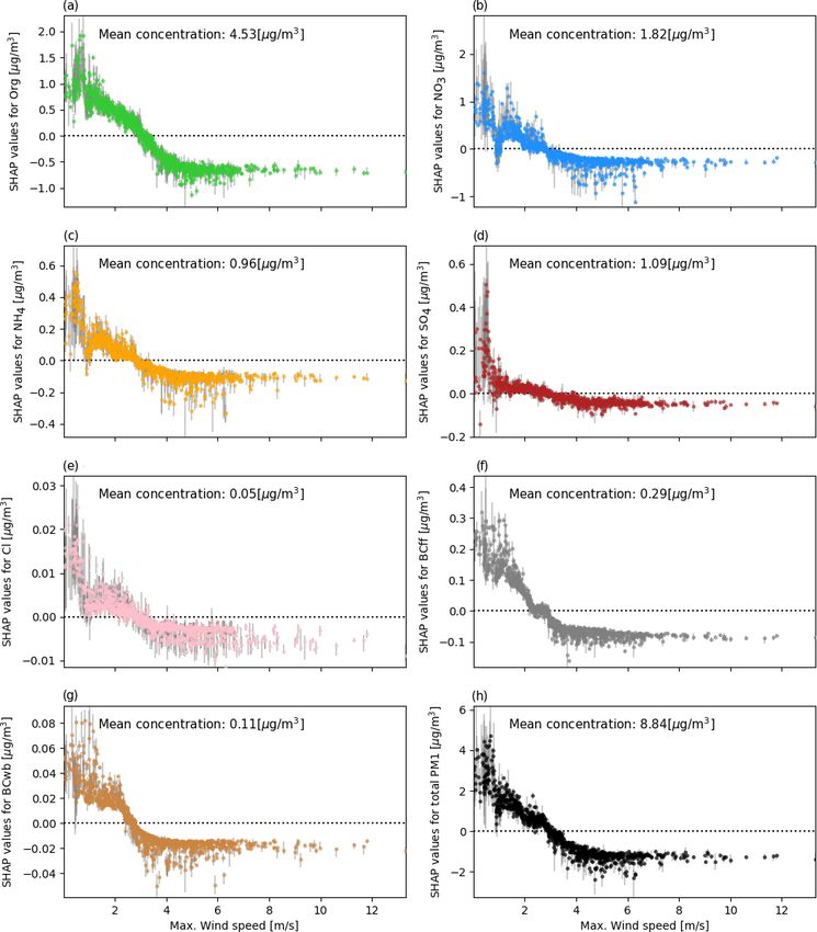
R. Stirnberg et al.: Meteorology-driven variability of air pollution                                                        3923

vide a deeper understanding of model decisions than the rela-     BCwb, BCff, and total PM1 show small spread, Cl− and
tively widely used partial dependence plots (Friedman, 2001;      NO− 3 exhibit larger variations between model runs (indicated
Goldstein et al., 2015; Fuchs et al., 2018; Lundberg et al.,      by horizontal and vertical lines in Fig. 3). This suggests that
2019; McGovern et al., 2019; Stirnberg et al., 2020). Par-        while drivers of variations in BCff concentration are well
tial dependence plots show the global mean effect of an in-       covered by the model, this is less so in the case of Cl− and
put feature to the model outcome, while SHAP values quan-         NO− 3 . Possible reasons for this are that no explicit infor-
tify the feature contribution to each single model output, ac-    mation on anthropogenic emissions or chemical formation
counting for multicollinearity. Feature contributions are cal-    pathways are included in the models. Still, the model perfor-
culated from the difference in model outputs with that fea-       mance indicators highlight that a large fraction of the vari-
ture present, versus outputs for a retrained model without        ations in particle concentrations are explained by the mete-
the feature. Since the effect of withholding a feature depends    orological variables used as model inputs. Performances of
on other features in the model due to interactive effects be-     model iterations of the species-specific and total PM1 are
tween the features, differences are computed for all possible     generally similar, suggesting a robust model outcome.
feature subset combinations of each data instance (Lundberg          The mean input feature importance, ordered from high to
and Lee, 2017).                                                   low, of the total PM1 model run by means of the SHAP fea-
   Summing up SHAP values for each input feature at a sin-        ture attribution values is shown in Fig. 4. The NO− 3 fraction
gle time step yields the final model prediction. SHAP val-        of the previous day has the highest impact on the model,
ues can be negative since SHAP values are added to the base       followed by temperature, wind direction information, and
value, which is the mean prediction when taking into account      MLH. To some extent, NO−     3 fraction can be related to PM1
all possible input feature combinations. Negative (positive)      mass concentrations (Petit et al., 2015; Beekmann et al.,
SHAP values reduce (raise) the prediction below (above) the       2015). This means that the higher the PM1 levels one day, the
base value. The higher the absolute SHAP value of a fea-          greater the chances of having higher PM1 levels the next day
ture, the more distinct is the influence of that feature on the   (see Fig. B1). Lower wind speeds generally lead to higher
model predictions. The sum of all SHAP values at one time         particle concentrations (see Fig. B2) due to a lack of disper-
step yields the final prediction of PM1 concentrations. An        sion (Sujatha et al., 2016). Temperature, MLH, and wind di-
example of breaking down a model prediction into feature          rection require an in-depth analysis, as changes of these vari-
contributions using SHAP values is shown schematically in         ables cause nonlinear responses in PM1 predictions, which
Fig. 2. The computation of traditional Shapley regression val-    also vary between species.
ues is time consuming, since a large number of all possible
feature combinations have to be included. The SHAP frame-         4.2     Influence of meteorological input features on
work for tree-based models allows a faster computation com-               modelled particle species and total PM1
pared to full Shapley regression values while maintaining                 concentrations
a high accuracy (Lundberg and Lee, 2017; Lundberg et al.,
2019) and is therefore used here. The SHAP Python imple-          To gain insights into relevant processes governing particle
mentation is used for the computation of SHAP values (https:      concentrations at SIRTA, the contribution of input features
//github.com/slundberg/shap, last access: 15 March 2021).         on species and total PM1 concentration outcomes from the
   The interactions of input features contribute to the model     statistical model, i.e. the SHAP values, are plotted as a func-
output and thus reflect empirical patterns that are important     tion of absolute feature values (Figs. 5–7). The contribution
to deepen the process understanding. Interactive effects are      of an input feature to each (local) prediction of the species or
defined as the difference between the SHAP values for one         total PM1 concentrations is shown while taking into account
feature when a second feature is present and the SHAP values      intra-model variability. Intra-model variability of SHAP val-
for the one feature when the other feature is absent (Lundberg    ues, i.e. different SHAP value attributions for the same fea-
et al., 2019).                                                    ture value within one model, is shown by the vertical distri-
                                                                  bution of dots for absolute input feature values. Intra-model
                                                                  variability is caused by interactions of the different model
4     Results and discussion                                      input features.

4.1    Model performance                                          4.2.1    Influence of temperature

The performance of the species and total PM1 models, each         The impact of ambient air temperature on modelled species
with 10 model iterations (of which each has different hy-         concentrations is highly non-linear (Fig. 5). All species show
perparameters) is assessed by comparing the coefficient of        increased contributions to model outcomes at temperatures
determination (R 2 ) and normalized root mean square error        below ∼ 4 ◦ C while the contribution of high temperatures on
(NRSME) for the independent test data that were withheld          model outcomes differs substantially between species. The
during the training process (Fig. 3). While the models for        statistical model is able to reproduce well-known character-

https://doi.org/10.5194/acp-21-3919-2021                                            Atmos. Chem. Phys., 21, 3919–3948, 2021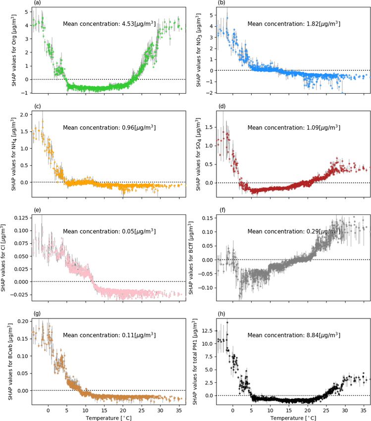
3924                                                           R. Stirnberg et al.: Meteorology-driven variability of air pollution

Figure 2. Conceptual figure illustrating the interaction of SHAP values and model output. Starting with a base value, which is the mean pre-
diction if all data points are considered, positive SHAP values (blue) increase the final prediction of total and speciated PM1 concentrations,
while negative SHAP values (red) decrease the prediction. The sum of all SHAP values for each input feature yields the final prediction.
Depending on whether positive or negative SHAP values dominate, the prediction is higher or lower than the base value (Lundberg et al.,
2018). Adapted from https://github.com/slundberg/shap (last access: 15 March 2021).

Figure 3. Performance indicators for 10 model iterations: coefficient of determination R 2 against normalized root mean squared error
                                                                                 2−
(NRMSE) for the separate species models (Org: organics, NH+                                      −            −
                                                             4 : ammonium, SO4 : sulfate, NO3 : nitrate, Cl : chloride, BCff: black
carbon from fossil fuel combustion, and BCwb: black carbon from wood burning), and the total PM1 model. Vertical and horizontal lines
indicate the maximum spread in R 2 and NRMSE, respectively, between the 10 model iterations.

istics of species concentration variations related to temper-             (Gen et al., 2019). Dawson et al. (2007) reported an increase
ature. For example, sulfate formation is enhanced with in-                of 34 ng/m3 K for PM2.5 concentrations using a CTM. The
creasing temperatures (Fig. 5d) due to an increased oxida-                increase in sulfate at low ambient temperatures as suggested
tion rate of SO2 (see Dawson et al., 2007; Li et al., 2017)               by Fig. 5d is not reported in this study. It is likely linked
and strong solar irradiation due to photochemical oxidation               to increased aqueous-phase particle formation in cold and

Atmos. Chem. Phys., 21, 3919–3948, 2021                                                      https://doi.org/10.5194/acp-21-3919-2021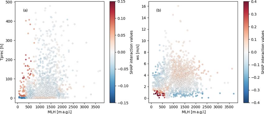
R. Stirnberg et al.: Meteorology-driven variability of air pollution                                                               3925

Figure 4. Ranked median SHAP values of the model input features, i.e. the average absolute value that a feature adds to the final model
outcome, referring to the total PM1 model [µg/m3 ] (Lundberg et al., 2018). Horizontal lines indicate the variability between model runs.

foggy situations (Rengarajan et al., 2011; Petetin et al., 2014;       tributions to modelled total PM1 concentrations of up to
Cheng et al., 2016). Considerable local formation of nitrate           12 µg/m3 . The spread of SHAP values between model iter-
at low temperatures (Fig. 5b) is consistent with results from          ations is generally higher for low temperatures (vertical grey
previous studies in western Europe, and enhanced formation             bars in Figs. 5–7), where SHAP values are of greater magni-
of ammonium nitrate at lower temperatures (Fig. 5c) by the             tude, but in all cases the signal contained in the feature con-
shifting gas-particle equilibrium is a well-known pattern (e.g.        tributions far exceeds the spread between model runs.
Clegg et al., 1998; Pay et al., 2012; Bressi et al., 2013; Petetin
et al., 2014; Petit et al., 2015). The increase in organic mat-        4.2.2   Influence of the mixed layer height (MLH)
ter and BCwb concentrations at low temperatures (Fig. 5g)
is likely related to the emission intensity, as biomass burning
                                                                       Variations in MLH can have a substantial impact on near-
is often used for domestic heating in the study area (Favez
                                                                       surface particle concentrations, as the mixed layer is the at-
et al., 2009; Sciare et al., 2010; Healy et al., 2012; Jiang et al.,
                                                                       mospheric volume in which the particles are dispersed (see
2019). In addition, organic matter concentrations are linked
                                                                       Klingner and Sähn, 2008; Dupont et al., 2016; Wagner and
to the condensation of semi-volatile organic species at low
                                                                       Schäfer, 2017). The effect of MLH variations on modelled
temperatures (Putaud et al., 2004; Bressi et al., 2013). The
                                                                       particle concentrations is highly nonlinear and varies in mag-
sharp increase in modelled concentrations of organics above
                                                                       nitude for all species (Fig. 6). Similar to the patterns observed
25 ◦ C (Fig. 5a) could be due to enhanced biogenic activity
                                                                       for temperature SHAP values, the inter-model variation of
leading to a rise in biogenic emissions and secondary aerosol
                                                                       predictions is highest for low MLHs where predicted particle
formation (Guenther et al., 1993; Churkina et al., 2017; Jiang
                                                                       concentrations have the highest variation. For predicted to-
et al., 2019).
                                                                       tal PM1 concentrations, the maximum positive contribution
   The contribution of temperature on modelled total PM1
                                                                       of the MLH is as high as 5.5 µg/m3 while negative contri-
concentrations (Fig. 6h) is consistent with the response pat-
                                                                       butions can amount to −2 µg/m3 . While the maximum influ-
terns to changes in temperatures described for the individual
                                                                       ence of MLH is lower than the maximum influence deter-
species in Fig. 6a–g, with positive contributions at both low
                                                                       mined for air temperature, the frequency of shallow MLH is
(< 4 ◦ C) and high air temperatures (> 25 ◦ C). For temper-
                                                                       far greater than that of the minimum temperatures that have
atures below freezing, the model allocates maximum con-
                                                                       the largest effect (Figs. 5d and 6d). Contributions of MLH

https://doi.org/10.5194/acp-21-3919-2021                                                 Atmos. Chem. Phys., 21, 3919–3948, 2021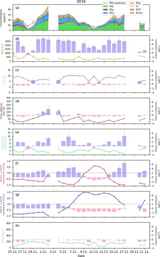
3926                                                           R. Stirnberg et al.: Meteorology-driven variability of air pollution

Figure 5. Air temperature SHAP values (contribution of temperature to the prediction of species and total PM1 concentrations [µg/m3 ] for
each data instance) vs. absolute air temperature [◦ C]. Inter-model variability of allocated SHAP values is shown as the variance of predicted
values between the 10 model iterations and plotted as vertical grey bars. The dotted horizontal line indicates the transition from positive to
negative SHAP values.

Atmos. Chem. Phys., 21, 3919–3948, 2021                                                     https://doi.org/10.5194/acp-21-3919-2021
R. Stirnberg et al.: Meteorology-driven variability of air pollution                                                            3927

to predicted particle concentrations are highest for very shal-     continental Europe and/or the Paris metropolitan area un-
low mixed layers due to the accumulation of particles close         der high-pressure system conditions versus cleaner marine
to the ground (Dupont et al., 2016; Wagner and Schäfer,             air masses during southwesterly flow (Bressi et al., 2013; Pe-
2017). In addition to causing particles to accumulate near          tetin et al., 2014; Petit et al., 2015; Srivastava et al., 2018).
the surface, low MLH can also provide effective pathways            Increased concentrations of organic matter are predicted for
for local new particle formation. Secondary pollutants, such        northerly, northeasterly, and easterly winds. These patterns
as ammonium nitrate, are increased at low MLHs when con-            suggest a significant contribution of advected organic parti-
ditions favourable to their formation usually coincide with         cles from a specific wind sector. This is in agreement with
reduced vertical mixing (i.e. low temperatures, often in com-       the findings of Petetin et al. (2014) who estimated that 69 %
bination with high RH; Pay et al., 2012; Petetin et al., 2014;      of the PM2.5 organic matter fraction is advected by north-
Dupont et al., 2016; Wang et al., 2016). BC concentrations,         easterly winds, which is related to advected particles from
on the other hand, are dominated by primary emissions, as           wood burning sources in the Paris region and SOA forma-
is a substantial fraction of organic matter (Petit et al., 2015).   tion along the transport trajectories. While Petit et al. (2015)
Hence, the accumulation of these particles during low buoy-         did not find a wind direction dependence of organic mat-
ancy conditions can explain the strong influence of MLH on          ter measured at SIRTA using wind regression, they reported
BCwb and BCff. A relatively distinct transition from posi-          the regional background of organic matter to be of impor-
tive contributions during shallow boundary layer conditions         tance. Comparing upwind rural stations to urban sites, Bressi
(∼ 0–800 m) towards negative contributions at high MLHs             et al. (2013) concluded organic matter is largely driven by
is evident for all species except SO2−                   2−
                                      4 . Modelled SO4 con-         mid-range to long-range transport. Influences on the SO2−      4 -
centrations show a less distinct response to changes in MLH         model are highest for northeastern and eastern wind di-
as they are largely driven by gaseous precursor sources and         rection, which aligns with previous findings by Pay et al.
particle advection, both rather independent of MLH (Pay             (2012), Bressi et al. (2014), and Petit et al. (2017), who iden-
et al., 2012; Petit et al., 2014, 2015), so that the accumu-        tified the Benelux region and western Germany as strong
lation effect is less important. The increase of SO2−4 concen-      emitters of sulfur dioxide (SO2 ). SO2 can be transformed
trations with higher MLHs (&1500 m a.g.l.) could be linked          to particulate SO2−   4 (Pay et al., 2012) while being trans-
to the effective transport of SO2− 4 and its precursor SO2 .        ported towards the measurement site. Nitrate concentrations
In agreement with results from previous studies focusing on         are affected by long-range transport from continental Europe
PM10 (Grange et al., 2018; Stirnberg et al., 2020) or PM2.5         (Benelux, western Germany), which are advected towards
(Liu et al., 2018), SHAP values do not change much for MLH          SIRTA from northeastern directions (Petetin et al., 2014; Pe-
above ∼ 800–900 m; i.e. boundary layer height variations            tit et al., 2014). It is to be expected that the influence of mid-
above this level do not influence submicron particle con-           range to long-range transport on the particle observations at
centrations. Positive contributions of MLHs above ∼ 800–            SIRTA is rather substantial, with most high-pollution days af-
900 m on predicted PM1 concentrations, as visible in Fig. 6         fected by particle advection from continental Europe (Bressi
for some species, have been previously reported by Grange           et al., 2013). Concerning BCff and BCwb, model results sug-
et al. (2018), who relate this pattern to enhanced secondary        gest a dependence on wind direction during northwestern
aerosol formation in a very deep and dry boundary layer. The        to northeastern inflow. Although BC concentrations are ex-
positive influence of high MLHs on species that are partly          pected to be largely determined by local emissions (Bressi
secondarily formed, e.g. SO2−  4 and Org, could be explained        et al., 2013), e.g. from local residential areas, a substantial
following this argumentation. The increase in SHAP values           contribution of imported particles from wood burning and
observed for BCff at high MLHs could be also related to             traffic emissions from the Paris region (Laborde et al., 2013;
secondary aerosol formation processes, causing an “encap-           Petetin et al., 2014) and continental sources is likely (Petetin
sulation” of BC within a thick coating of secondary aerosols        et al., 2014).
(Zhang et al., 2018).
                                                                    4.2.4   Influence of feature interactions
4.2.3   Influence of wind direction
                                                                    Pairwise interaction effects, where the effect of a specific
To analyse the contribution of wind direction to predicted          predictor on the total PM1 prediction is dependent on the
particle concentrations, SHAP values of normalized 3 d mean         state of a second predictor, are analysed in the model. Strong
u and v wind components were added up and transformed               pairwise interactive effects are found between MLH vs. time
to units of degrees (Fig. 7). Generally, wind direction has         since last precipitation and MLH vs. maximum wind speed
a positive contribution to the model outcome when winds             and shown in Fig. 8a and b. SHAP interaction effects be-
from the northern to northeastern sectors prevail, while neg-       tween MLH and time since last precipitation are most pro-
ative contributions are evident for southwesterly directions.       nounced for MLHs below ∼ 500 m a.g.l. (Fig. 8a). Interac-
Given the location of the measurement site, this pattern un-        tion values are negative for low MLHs paired with time since
doubtedly reflects the advection of particles emitted from          last precipitation close to zero hours. With increasing time

https://doi.org/10.5194/acp-21-3919-2021                                             Atmos. Chem. Phys., 21, 3919–3948, 2021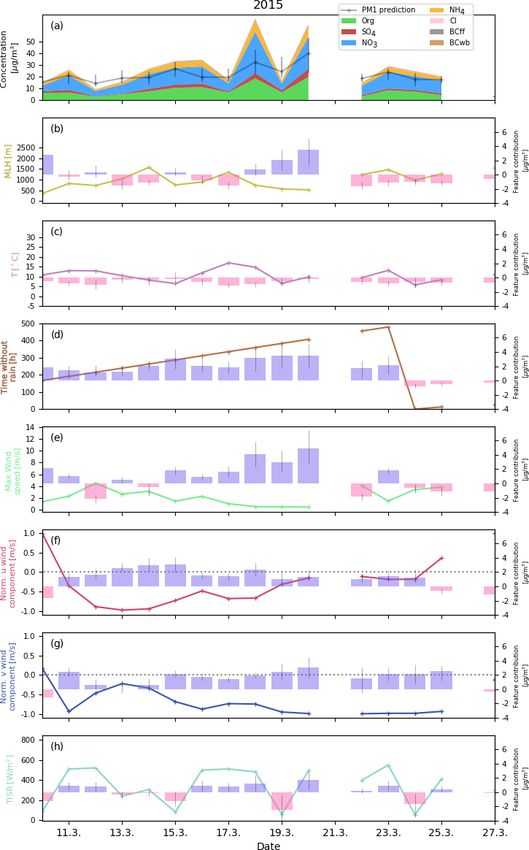
3928                                                      R. Stirnberg et al.: Meteorology-driven variability of air pollution

Figure 6. As Fig. 5 for MLH SHAP values (contribution of MLH to the prediction of species and total PM1 for each data instance) vs.
absolute MLH values [m. a.g.l.].

Atmos. Chem. Phys., 21, 3919–3948, 2021                                              https://doi.org/10.5194/acp-21-3919-2021
R. Stirnberg et al.: Meteorology-driven variability of air pollution                                                                3929

Figure 7. As Fig. 5 for wind direction SHAP values (contribution of 3 d mean wind direction to the prediction of species and total PM1 for
each data instance) vs. absolute wind direction [◦ ].

https://doi.org/10.5194/acp-21-3919-2021                                                 Atmos. Chem. Phys., 21, 3919–3948, 2021
3930                                                      R. Stirnberg et al.: Meteorology-driven variability of air pollution

since last precipitation, interaction effects become positive,     low MLHs, low wind speeds, a high average NO−          3 fraction
thus increasing the contribution of Tprec and MLH to the           of the previous day, and negative u (i.e. winds from the east)
model outcome. An explanation of this pattern concerning           and v (i.e. winds from the north) wind components. In win-
underlying processes could be that due to the lack of pre-         ter, the PM1 composition shows a relatively large fraction
cipitation, a higher number of particles is available in the       of nitrates, which is increased during high-pollution situa-
atmosphere for accumulation, hence increasing the accumu-          tions (Fig. 9, lower panel). High concentrations of nitrate in
lation effect of a shallow MLH. In case of recent precipi-         winter can be linked to advection or to enhanced formation
tation, the accumulation effect of a shallow MLH is weak-          due to the temperature-dependent low volatility of ammo-
ened. For higher MLHs, interactive effects with time since         nium nitrate (Petetin et al., 2014). The organic matter fraction
the last precipitation event are marginal. Interactive effects     is slightly decreased during high-pollution situations. MLH
between MLH and wind speed are shown in Fig. 8b. Posi-             and maximum wind speed influences on high-pollution situ-
tive SHAP values for maximum wind speeds below ∼ 2 m/s             ations are linked to low-ventilation conditions which are very
reflect stable situations, favouring the accumulation of par-      frequent in winter (Dupont et al., 2016). Positive influences
ticles, whereas high wind speeds enhance the ventilation of        of wind direction for inflow from the northern and eastern
particles (Sujatha et al., 2016). This can also be deduced from    sectors are dominant during high-pollution situations while
Fig. 8b, which shows increased SHAP values for low wind            inflow from the southern and western sectors prevails during
speeds in combination with a low MLH. Low wind speeds              average-pollution situations (see Fig. 7; Bressi et al., 2013;
combined with a high MLH (&1000 m a.g.l.), on the other            Petetin et al., 2014; Srivastava et al., 2018). Note that the time
hand, result in decreased SHAP values. Similarly, low MLHs         since the last precipitation is increased during high-pollution
combined with higher wind speeds (&2 m/s) also decrease            situations, but the effects on the model outcome is weak. This
predictions of total PM1 concentrations. High MLHs in com-         suggests that lack of precipitation is not a direct driver of
bination with high wind speeds, however, reduce SHAP val-          modelled total PM1 concentrations but increases the contri-
ues. A physical explanation of this pattern could be the more      bution of other input features (see Fig. 8a) or is a meaningful
effective transport of SO2− 4 and its precursor SO2 as well as     factor in only some situations.
ammonium nitrate under high-MLH conditions and stronger               Summer total PM1 composition (Fig. 10) is characterized
winds (Pay et al., 2012). Maximum wind speed and time              by a larger fraction of organics compared to the winter sea-
since last precipitation (plot not shown here) interact in a       son (Fig. 9). As a considerable fraction of organic matter is
similar way. The positive effect of low wind speeds on the         formed locally (Petetin et al., 2014), the increased propor-
model outcome is increasing with increasing time since last        tion of organics could be due to more frequent stagnant syn-
precipitation.                                                     optic situations that may limit the advection of transported
                                                                   SIA particles. In addition, the positive SHAP values of so-
4.3    Meteorological conditions of high-pollution events          lar irradiation and temperature highlight that the solar irradi-
                                                                   ation stimulates transformation processes and increases the
To further identify conditions that favour high-pollution          number of biogenic SOA particles (Guenther et al., 1993;
episodes, the data set is split into situations with excep-        Petetin et al., 2014). As mean temperatures are highest in
tionally high total PM1 concentrations (> 95th percentile)         summer, positive temperature SHAP values are associated
and situations with typical concentrations of total PM1 (in-       with increased organic matter concentrations (Fig. 5). The
terquartile range, IQR). This is done for the meteorological       higher importance (i.e. higher SHAP values) of time since
summer and winter seasons to contrast dominant drivers be-         the last precipitation event during high-pollution situations
tween these seasons. Mean SHAP values refer to the total           points to an accumulation of particles in the atmosphere. Dry
PM1 model; corresponding input feature distributions and           situations can also enhance the emission of dust over dry
species fractions for the two subgroups are aggregated sea-        soils (Hoffmann and Funk, 2015). The negative influences
sonally. This allows for a quantification of seasonal feature      of MLH during both typical and high-pollution situations re-
contributions to average or polluted situations.                   flects seasonality, as afternoon MLHs in summer are usually
   Figures 9 and 10 show mean SHAP values for typical (left)       too high to have a substantial positive impact on total PM1
and high-pollution (right) situations in the upper panel. The      concentrations (see Fig. 6). MLH is thus not expected to be a
distribution of SHAP values are shown as box plots for each        driver of day-to-day variations of summer total PM1 concen-
feature. Absolute feature value distributions are given in the     trations. Note that the average MLH is higher during high-
bottom of the figure. In the lowest subpanel, the chemical         pollution situations, which likely points to increased forma-
composition of the total PM1 concentration for each sub-           tion of SO2−4 (see Fig. 6).
group is shown. The largest contributor to high-pollution sit-
uations in winter is air temperature (Fig. 9). SHAP values for     4.4   Day-to-day variability of selected pollution events
temperature are substantially increased during high-pollution
situations, when temperatures are systematically lower. Fur-       Analysing the combination of SHAP values of the various
ther contributing factors to high-pollution situations are the     input features on a daily basis allows for direct attribution

Atmos. Chem. Phys., 21, 3919–3948, 2021                                              https://doi.org/10.5194/acp-21-3919-2021
R. Stirnberg et al.: Meteorology-driven variability of air pollution 3931
Figure 8. MLH vs. (a) time since last precipitation and (b) maximum wind speed, coloured by the SHAP interaction values for the respective
features.
Table 1. Statistics for typical PM1 concentrations (mean, median, IQR) and high-pollution concentrations (> 95th percentile).
PM1 concentrations Mean Median Interquartile range 95th percentile
Winter (DJF) 11.1 µg/m3 6.3 µg/m3 2.7–15.4 µg/m3 34.3 µg/m3
Summer (JJA) 7.5 µg/m3 6.0 µg/m3 3.5–10.1 µg/m3 18.2 µg/m3
of the respective implications for modelled total PM1 con- (strong negative u component, weak negative v component)
centrations (Lundberg et al., 2020). Here, four particular pol- on 19 January. The combined effects of these changes lead
lution episodes are selected to analyse the model outcome to a marked increase in total modelled PM1 concentrations,
with respect to physical processes (Figs. 11–14). The ex- peaking at ∼37 µg/m3 on 20 January. On the following days,
amples highlight the advantages but also the limitations of temperatures increase steadily; thus the contribution of tem-
the interpretation of the statistical model results. The high- perature decreases. At the same time, although values of
pollution episodes took place in winter 2016 (10–30 Jan- MLH remain almost constant, the contribution of MLH drops
uary and 25 November–25 December), spring 2015 (11– substantially from ∼ 5 to ∼ 2 µg/m3 . This is due to interac-
31 March), and summer 2017 (8–28 June). tive effects between MLH and the features wind speed, time
since last precipitation, and normalized v wind component.
4.4.1 January 2016 All of these features increase the contribution of MLH on
20 January but decrease its contribution on 21–23 January.
Prior to the onset of the high-pollution episode in January The physical explanation behind this pattern would be that
2016 (Fig. 11), the situation is characterized by MLHs at a lack of wet deposition and low wind speeds increase par-
approximately 1000 m, temperatures above freezing (∼ 5– ticle numbers in the atmosphere, while inflows from north-
10◦ C), frequent precipitation, and winds from the southwest. easterly directions increase particle numbers in the atmo-
The organic matter fraction dominates the particle speciation. sphere. Given that there is now a large number of particles
The episode itself is reproduced well by the model. Accord- present, the accumulation effect of a low MLH is more effi-
ing to the model results, the event is largely temperature- cient. The high-pollution episode ceases after a shift to south-
driven, i.e. SHAP values of temperature explain a large frac- eastern winds and the increasing temperatures. The pollution
tion of the total PM1 concentration variation (note the ad- episode is characterized by a relatively large fraction of NO−3
justed y axis of the temperature SHAP values). On 18 Jan- and NH+ 4 , which explains the strong feature contribution of
uary, temperatures drop below freezing, coupled with a de- temperature to the modelled total PM1 concentration, as the
crease in MLH. As a consequence, both modelled and ob- abundance of these species is temperature dependent (see
served PM1 concentrations start to rise. A further increase Fig. 5) and points to a large contribution of locally formed
in total PM1 concentrations is driven by a sharp transition inorganic particles. Still, the contribution of wind direction
from stronger southwestern to weaker northeastern winds and speed also suggests that advected secondary particles and
https://doi.org/10.5194/acp-21-3919-2021 Atmos. Chem. Phys., 21, 3919–3948, 20213932 R. Stirnberg et al.: Meteorology-driven variability of air pollution Figure 9. Mean feature contributions (i.e. SHAP values) for situations with low total PM1 concentrations (left) and situations with high pollution (right), respectively, during winter (December, January, February). Respective ranges of SHAP values by species are shown as box plots, with median (bold line), 25–75th percentile range (boxes), and 10–90th percentile range (whiskers). Both training and test data are included. Absolute feature value distributions (given as normalized frequencies) as well as the chemical composition of the total PM1 concentration are shown in the subpanels. Colours of the box plots correspond to colours in the feature distribution subpanels. SHAP values of the input features u_norm_3d and u_norm as well as v_norm_3d and v_norm were merged to “u_norm, merged” and “v_norm, merged” to achieve better transparency. Atmos. Chem. Phys., 21, 3919–3948, 2021 https://doi.org/10.5194/acp-21-3919-2021
R. Stirnberg et al.: Meteorology-driven variability of air pollution                                                                   3933

Figure 10. As Fig. 9 for mean feature contributions (i.e. SHAP values) for situations with low total PM1 concentrations (left) and situations
with high-pollution (right), respectively, during summer (July, June, August).

https://doi.org/10.5194/acp-21-3919-2021                                                   Atmos. Chem. Phys., 21, 3919–3948, 2021
3934 R. Stirnberg et al.: Meteorology-driven variability of air pollution
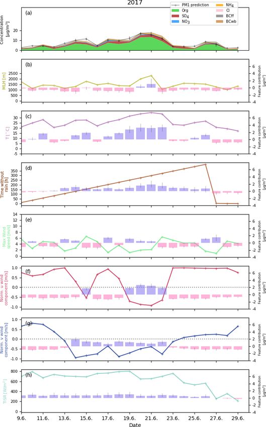
their build-up in the boundary layer are relevant factors dur- tions. A lack of precipitation (no rain for a period of more
ing the development of the high-pollution episode (Petetin than 2 weeks) and high temperatures also contribute to the
et al., 2014; Petit et al., 2014; Srivastava et al., 2018). total PM1 concentrations during this episode. While solar
irradiation and time since last precipitation are associated
4.4.2 December 2016 with positive SHAP values throughout this period, air tem-
perature only has a positive contribution when exceeding
A high-pollution episode with several peaks of total PM1 is ∼ 25 ◦ C. This aligns with patterns shown in Fig. 5, where in-
observed in November and December 2016. The first peak creased concentrations of organic matter and SO42− are iden-
on 26 November is followed by an abrupt minimum in to- tified for high temperatures. Peak total PM1 concentrations
tal PM1 concentrations on 28 November, and a build-up of of ∼17 µg/m3 are observed on 20 and 21 June. A change in
pollution in a shallow boundary layer towards the second the east–west wind component from western to eastern in-
peak on 2 December with total PM1 concentrations exceed- flow directions in conjunction with an increase in tempera-
ing 40 µg/m3 . In the following days, total PM1 concentra- tures to above 30 ◦ C are the drivers of the modelled peak in
tions continuously decrease, eventually reaching a second total PM1 concentrations. MLH is also increased with values
minimum on 11 December. A gradual increase in total PM1 ∼ 2000 m a.g.l., which are associated with slightly positive
concentrations follows, resulting in a third (double-)peak to- SHAP values. This observation fits with findings described
tal PM1 concentration on 17 December. Total PM1 concen- in Sect. 4.2.2 and is likely linked to enhanced secondary par-
trations drop to lower levels afterwards. Throughout the 3.5- ticle formation (Megaritis et al., 2014; Jiang et al., 2019). As
week-long episode, high pollution is largely driven by shal- suggested by response patterns of species to changes in MLH
low MLH (.500 m) and weak north-northeasterly winds, shown in Fig. 7, this effect is linked to an increase in SO2− 4
i.e. a regime of low ventilation associated with high pres- concentrations. The main fraction of the peak total PM1 val-
sure conditions favourable for emission accumulation and ues, however, is linked to an increase in organic matter con-
possibly some advection of polluted air from the Paris re- centrations due to the warm temperatures (see Fig. 5).
gion. During the brief periods with lower total PM1 con-
centrations, these conditions are disrupted by a higher MLH 4.4.4 March 2015
(∼ 28 November) or a change in prevailing winds (∼ 11 De-
cember). In contrast to the pollution episode in January 2016, High particle concentrations are measured in early March
this December 2016 episode is not driven by temperature 2015 with high day-to-day variability. This modelled course
changes. Temperatures range between ∼ 5–12◦ C and have of the pollution episode is chosen to compare results to pre-
a minor contribution to predicted total PM1 concentrations vious studies focusing on the evolution of this episode (Petit
(see also Fig. 5), emphasizing the different processes caus- et al., 2017; Srivastava et al., 2018). The episode is charac-
ing air pollution in the Paris region. Note that the model is terized by high fractions of SIA particles, in particular SO2−
4 ,
not able to fully reproduce the pollution peak on 2 Decem- NH+ 4 , and NO −
3 (Fig. 14a) and similar concentrations ob-
ber, which may be indicative of missing input features in the served at multiple measurement sites in France (Petit et al.,
model. Judging from the PM1 species composition during 2017). Contributions of local sources are low, and much of
this time (relatively high fraction of NO−3 and BC), it seems the episode is characterized by winds blowing in from the
likely that missing information on particle emissions may be northwest, advecting aged SIA particles (Petit et al., 2017;
the reason for the difference between modelled and observed Srivastava et al., 2018) and organic particles of secondary
total PM1 concentration. origin (Srivastava et al., 2019) towards SIRTA. A widespread
scarcity of rain probably enhanced the large-scale forma-
4.4.3 June 2017 tion of secondary pollution across western Europe (in par-
ticular western Germany, the Netherlands, Luxemburg; Petit
A period of above-average total PM1 concentrations oc- et al., 2017), which were then transported towards SIRTA.
curred in June 2017. The episode is very well reproduced This is reflected by the SHAP values of the u and v wind
by the model, suggesting a strong dependence of the ob- components, which are positive throughout the episode (see
served total PM1 concentration to meteorological drivers. Al- Fig. 14g and h). Concentration peaks of total PM1 are mea-
though absolute total PM1 concentrations are substantially sured on 18 and 20 March. Both peaks are characterized by a
lower than during the previously described winter pollution rapid development of total PM1 concentrations. As described
episodes, the event is still above average for summer pollu- in Petit et al. (2017), these strong daily variations of total
tion levels. Organic matter particles dominate the PM1 frac- PM1 , which are mainly driven by the SIA fraction, could be
tion throughout the episode, with a relatively high SO2− 4 due to varying synoptic cycles, especially the passage of cold
fraction. Conditions during this episode are characterized fronts. The influence of MLH and temperature is relatively
by strong solar irradiation (positive SHAP values) and high small, which is consistent with the high influence of advec-
MLHs (mostly negative SHAP values), which show low day- tion on total PM1 concentrations during the episode. The
to-day variability and reflect characteristic summer condi- exceptional character of the episode (see Petit et al., 2017)
Atmos. Chem. Phys., 21, 3919–3948, 2021 https://doi.org/10.5194/acp-21-3919-2021You can also read