Greenland ice sheet mass balance from 1840 through next week
←
→
Page content transcription
If your browser does not render page correctly, please read the page content below
Earth Syst. Sci. Data, 13, 5001–5025, 2021
https://doi.org/10.5194/essd-13-5001-2021
© Author(s) 2021. This work is distributed under
the Creative Commons Attribution 4.0 License.

                   Greenland ice sheet mass balance from 1840
                                through next week
          Kenneth D. Mankoff1 , Xavier Fettweis2 , Peter L. Langen3 , Martin Stendel4 , Kristian K. Kjeldsen1 ,
          Nanna B. Karlsson1 , Brice Noël5 , Michiel R. van den Broeke5 , Anne Solgaard1 , William Colgan1 ,
              Jason E. Box1 , Sebastian B. Simonsen6 , Michalea D. King7 , Andreas P. Ahlstrøm1 , Signe
                                       Bech Andersen1 , and Robert S. Fausto1
               1 Department   of Glaciology and Climate, Geological Survey of Denmark and Greenland (GEUS),
                                                      Copenhagen, Denmark
                  2 SPHERES research unit, Department of Geography, University of Liège, Liège, Belgium
                  3 Department of Environmental Science, iClimate, Aarhus University, Roskilde, Denmark
                                  4 Danish Meteorological Institute (DMI), Copenhagen, Denmark
                     5 Institute for Marine and Atmospheric Research, Utrecht University, the Netherlands
             6 Geodesy and Earth Observation, DTU Space, Technical University of Denmark, Lyngby, Denmark
                               7 Polar Science Center, University of Washington, Seattle, WA, USA

                                       Correspondence: Ken Mankoff (kdm@geus.dk)

                                     Received: 21 April 2021 – Discussion started: 26 April 2021
                        Revised: 13 August 2021 – Accepted: 20 September 2021 – Published: 29 October 2021

       Abstract. The mass of the Greenland ice sheet is declining as mass gain from snow accumulation is exceeded
       by mass loss from surface meltwater runoff, marine-terminating glacier calving and submarine melting, and
       basal melting. Here we use the input–output (IO) method to estimate mass change from 1840 through next week.
       Surface mass balance (SMB) gains and losses come from a semi-empirical SMB model from 1840 through 1985
       and three regional climate models (RCMs; HIRHAM/HARMONIE, Modèle Atmosphérique Régional – MAR,
       and RACMO – Regional Atmospheric Climate MOdel) from 1986 through next week. Additional non-SMB
       losses come from a marine-terminating glacier ice discharge product and a basal mass balance model. From
       these products we provide an annual estimate of Greenland ice sheet mass balance from 1840 through 1985
       and a daily estimate at sector and region scale from 1986 through next week. This product updates daily and
       is the first IO product to include the basal mass balance which is a source of an additional ∼ 24 Gt yr−1 of
       mass loss. Our results demonstrate an accelerating ice-sheet-scale mass loss and general agreement (coefficient
       of determination, r 2 , ranges from 0.62 to 0.94) among six other products, including gravitational, volume, and
       other IO mass balance estimates. Results from this study are available at https://doi.org/10.22008/FK2/OHI23Z
       (Mankoff et al., 2021).

1   Introduction                                                   discharge losses dominated. More recently, in the 2010s, all
                                                                   sectors lost mass, with some sectors losing mass almost en-
Over the past several decades, mass loss from the Greenland        tirely via negative SMB and others primarily due to discharge
ice sheet has increased (Khan et al., 2015; IMBIE Team,            (Fig. 1).
2019). Different processes dominate the regional mass loss            There are three common methods for estimating mass bal-
of the ice sheet, and their relative contribution has fluctuated   ance – changes in gravity (Barletta et al., 2013; Groh et al.,
in time (Mouginot and Rignot, 2019). For example, in the           2019; IMBIE Team, 2019; Velicogna et al., 2020), changes
1970s nearly all sectors gained mass due to positive surface       in volume (Simonsen et al., 2021a; Sørensen et al., 2011;
mass balance (SMB), except the northwestern sector, where

Published by Copernicus Publications.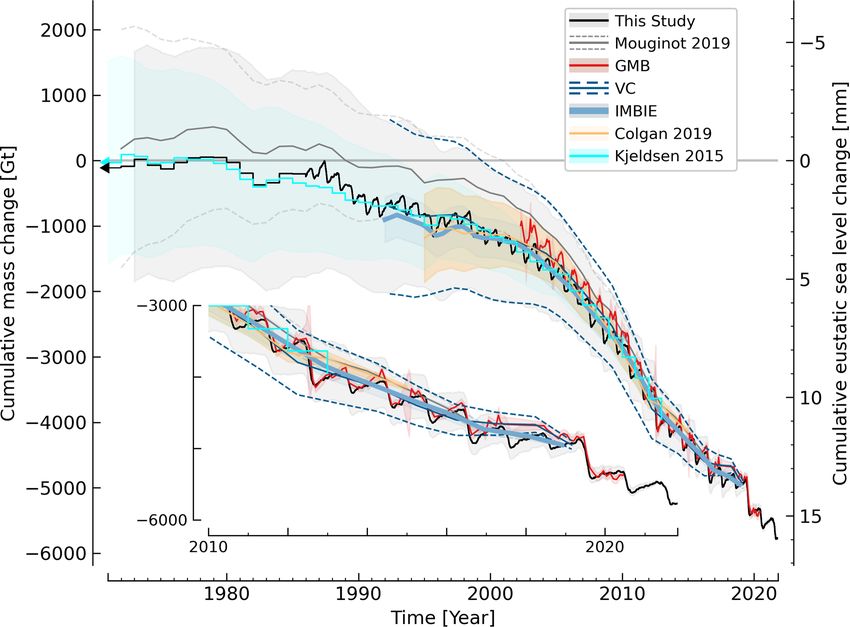
5002                                                    K. D. Mankoff et al.: Greenland mass balance 1840 through next week

Figure 1. Annual mass balance (black lines), surface mass balance (blue lines), and discharge plus basal mass balance (dashed grey) in
Gt yr−1 for each of the seven Mouginot and Rignot (2019) regions. The map shows both the named regions (Mouginot and Rignot, 2019)
and the numbered sectors (Zwally et al., 2012). Discharge gates are marked in black. Only recent (post-1986) data are shown because
reconstructed data are not separated into regions or sectors. Next week is defined as 1 November 2021 based on the date this document was
compiled.

Zwally and Giovinetto, 2011; Sasgen et al., 2012; Smith                year temporal resolution (when), and little information on the
et al., 2020), and the input–output (IO) method (Colgan et al.,        driving processes (how).
2019; Mouginot et al., 2019; Rignot et al., 2019; King et al.,            The IO method has a complex spatial resolution (where).
2020). Each provides some estimate of where, when, and                 The inputs typically come from regional climate models
how the mass is lost or gained, and each method has some               (RCMs) which can reach a spatial resolution of up to 1 km.
limitations. The gravity mass balance (GMB) estimate has               However, that spatial resolution is generally reduced in the
low ∼ 100 km spatial resolution (where), monthly tempo-                final output to sector or region scale – typically higher than
ral resolution (when), and little information on the processes         GMB but now lower resolution than VC. The IO temporal
contributing to changes in mass balance components (how).              resolution (when) is limited by ice velocity data updates,
The volume change (VC) mass balance estimate has ∼ 1 km                which for the past several years occur every 12 d year-round
spatial resolution (where), often provided at annual or multi-         after the launch of the Sentinel missions (Solgaard et al.,
                                                                       2021). The primary issue with the IO method is unknown

Earth Syst. Sci. Data, 13, 5001–5025, 2021                                              https://doi.org/10.5194/essd-13-5001-2021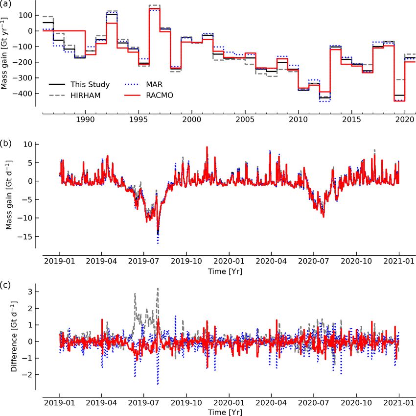
K. D. Mankoff et al.: Greenland mass balance 1840 through next week                                                      5003

ice thickness in some locations (e.g., Mankoff et al., 2020b).        – Region refers to the Mouginot and Rignot (2019) re-
Finally, the IO method can provide insight into the processes           gions (Fig. 1), expanded here to cover the RCM ice do-
(how) by distinguishing between changes caused by SMB                   mains.
(which may be due to changes in positive and/or negative
SMB components) vs. changes in other mass loss terms (e.g.,           – SMB is the surface mass balance from an RCM or the
calving). Our IO method is also the first IO product to include         average of multiple RCM SMBs. The use should be
the basal mass balance (Karlsson et al., 2021) – a term im-             clear from the context.
plicitly included in the GMB and VC methods but neglected
                                                                      – D is solid ice discharge. It includes both calving and
by all previous IO estimates.
                                                                        submarine melting at marine-terminating glaciers.
   In this work we introduce the new Programme for Moni-
toring of the Greenland ice sheet (PROMICE) Greenland ice             – BMB is the basal mass balance. It comes from geother-
sheet mass balance data set based on the IO method, updat-              mal flux (BMBGF ), frictional heating from ice velocity
ing the previous product from Colgan et al. (2019). We use              (BMBfriction ), and viscous heat dissipation (BMBVHD ).
the SMB field from one empirical model from 1840 through
1985 and three RCMs from 1986 onward. The combined                    – MB is the total mass balance including the BMB term
SMB field used here is comprised of positive SMB terms                  (Eq. 3).
(precipitation in the form of snowfall, rainfall, condensa-
tion/riming, and snow drift deposition) and negative SMB              – MB∗ is the mass balance not including the BMB term
terms (surface melt, evaporation, sublimation, and snow drift           (Eq. 4).
erosion). We also use the basal mass balance and an esti-
                                                                      – HIRHAM/HARMONIE, Modèle Atmosphérique Ré-
mate of dynamic ice discharge. Spatial resolution is effec-
                                                                        gional (MAR), and Regional Atmospheric Climate
tively per sector (Zwally et al., 2012) or region (Mouginot
                                                                        MOdel (RACMO) refer to the RCMs, which only pro-
and Rignot, 2019). Temporal resolution is annual from 1840
                                                                        vide SMB and runoff in the case of MAR. However,
through 1985 and effectively daily since 1986 – the RCM
                                                                        when referencing the different MB products, we use, for
fields are updated daily and forecasted through next week,
                                                                        example, “MAR MB” rather than repeatedly explicitly
and the discharge at marine-terminating glaciers is updated
                                                                        stating “MB derived from MAR SMB minus BMB and
every 12 d with ∼ 12 d resolution, interpolated to daily, and
                                                                        D”. The use should be clear from the context.
forecasted using historical and seasonal trends through next
week. Thus, this study provides a daily-updating estimate of
Greenland mass changes from 1840 through next week.               3    Product description

                                                                  The output of this work is two NetCDF files and two CSV
2    Terminology                                                  files containing a time series of mass balance and the com-
                                                                  ponents used to calculate mass balance. The only difference
We use the following terminology throughout the document.         between the two NetCDF files is the region of interest (ROI)
                                                                  – one for Zwally et al. (2012) sectors and one for Mouginot
    – This Study refers to the new results presented in this      and Rignot (2019) regions. Each NetCDF file includes the
      study.                                                      ice sheet mass balance (MB), MB per ROI (sector or region),
                                                                  MB per ROI per RCM, ice sheet SMB, SMB per ROI, ice
    – Recent refers to the new 1986 through next week daily
                                                                  sheet discharge (D), D per ROI, ice sheet BMB, and BMB per
      temporal resolution data at regional and sector scales.
                                                                  ROI. The CSV files contain a copy of the ice-sheet-summed
                                                                  data, one daily and one annual.
    – Reconstructed refers to the adjusted Kjeldsen et al.
                                                                     An example of the output is shown in Fig. 2a, which shows
      (2015) annual temporal resolution data at ice sheet scale
                                                                  mass balance for the entire Greenland ice sheet in addition
      used to extend this product from 1986 back through
                                                                  to SMB and D at annual resolution. Figure 2b shows an ex-
      1840. The 1986 through 2012 portion of the Kjeldsen
                                                                  ample of 2 years at daily temporal resolution. The ice-sheet-
      et al. (2015) data set is used only to adjust the recon-
                                                                  wide product includes data from 1840 through next week, but
      structed data and is then discarded.
                                                                  the sector and region-scale products only include data from
    – ROI (region of interest) refers to one or more of the ice   1986 through next week, because the 1840 through 1985 re-
      sheet sectors or regions (Fig. 1).                          constructed only exists at ice sheet scale (Fig. 1).

    – Sector refers to one of the Zwally et al. (2012) sectors    4    Data sources
      (Fig. 1), expanded here to cover the RCM ice domains
      which exist slightly outside these sectors in some loca-    This section introduces data products that exist prior to and
      tions.                                                      are external to this work (Table 1). In the following Methods

https://doi.org/10.5194/essd-13-5001-2021                                        Earth Syst. Sci. Data, 13, 5001–5025, 2021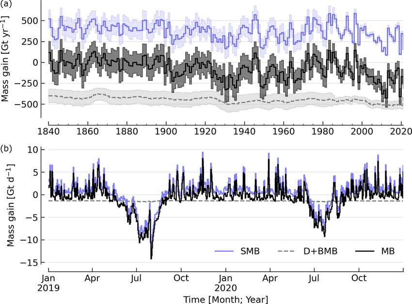
5004                                                    K. D. Mankoff et al.: Greenland mass balance 1840 through next week

Figure 2. Mass balance and its major components. (a) Annual average surface mass balance (blue line), discharge (gray dashed), and their
mass balance sum (black line). Here the discharge and basal mass balance (D + BMB) are shown with sign inverted (e.g., −1 × (D + BMB)).
(b) Same data at daily resolution and limited to 2019 and 2020.

section we introduce both the intermediate products we gen-           4.1.1   HIRHAM/HARMONIE
erate using these data sources and the final product that is the
output of This Study.
   The inputs to this work are the recent SMB fields from             The HIRHAM/HARMONIE product from the Danmarks
the three RCMs, the recent discharge from Mankoff et al.              Meteorologiske Institut (Danish Meteorological Institute;
(2020b) (data: Mankoff and Solgaard, 2020), and the recent            DMI) is based on an offline subsurface firn/SMB model
basal mass balance fields, of which BMBGF and BMBfriction             (Langen et al., 2017), which is forced with surface fluxes
are direct outputs from Karlsson et al. (2021) (data: Karlsson,       of energy (turbulent and downward-radiative) and mass
2021), but the BMBVHD calculations are redone here (see               (snow, rain, evaporation, and sublimation). These surface
Methods Sect. 5.3) using the MAR runoff field. The recon-             fluxes are derived from the HIRHAM5 regional climate
structed data (pre-1986) are surface mass balance and dis-            model for the reconstructed part of the simulation and from
charge from Kjeldsen et al. (2015) (data: Box et al., 2021)           DMI’s operational numerical weather forecast model HAR-
but adjusted here using the overlapping period (see Methods           MONIE (Iceland–Greenland domain “B”, which covers Ice-
Sect. 5.4) and runoff from Kjeldsen et al. (2015) (data: Box          land, Greenland, and the adjacent seas) for the real-time part.
et al., 2021) as a proxy and scaled for BMBVHD (see Methods           HIRHAM5 is used until 31 August 2017, after which HAR-
Sect. 5.3).                                                           MONIE is used.
                                                                         The HIRHAM5 regional climate model (Christensen et al.,
4.1    Surface mass balance                                           2007) combines the dynamical core of the HIRLAM7 numer-
                                                                      ical weather forecasting model (Eerola, 2006) with physics
We use one reconstructed SMB from 1840 through 1985
                                                                      schemes from the ECHAM5 general circulation model
and three recent SMBs from 1986 through last month
                                                                      (Roeckner et al., 2003). In the Greenland setup employed
(HIRHAM/HARMONIE, MAR, and RACMO), two through
                                                                      here (Lucas-Picher et al., 2012), it has a horizontal resolu-
yesterday (HIRHAM/HARMONIE and MAR) and one
                                                                      tion of 0.05◦ ×0.05◦ on a rotated pole grid (corresponding to
through next week (MAR).
                                                                      5.5 km resolution) and 31 atmospheric levels. It is forced at
                                                                      6 h intervals on the lateral boundaries with horizontal wind
                                                                      vectors, temperature, and specific humidity from the ERA-
                                                                      Interim reanalysis (Dee et al., 2011). ERA-Interim sea sur-
                                                                      face temperatures and sea ice concentration are prescribed in

Earth Syst. Sci. Data, 13, 5001–5025, 2021                                             https://doi.org/10.5194/essd-13-5001-2021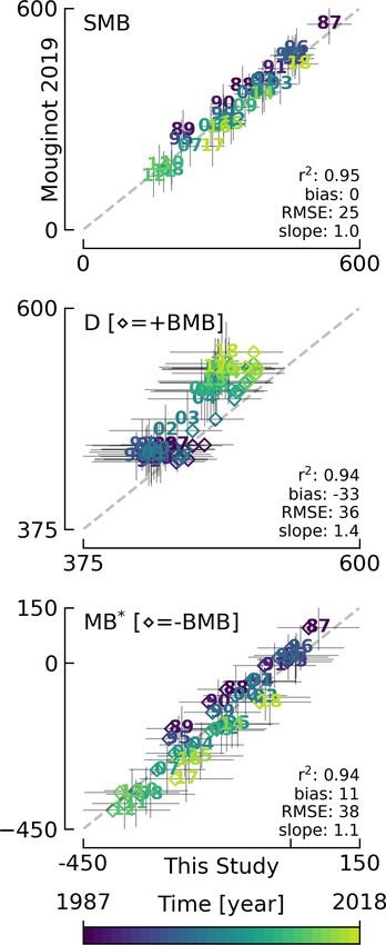
K. D. Mankoff et al.: Greenland mass balance 1840 through next week                                                                 5005

Table 1. Summary of data products used as inputs to This Study.

        Product                        Period                     Reference                Data/notes
        Reconstructed SMB              1840 through 1985          Kjeldsen et al. (2015)   Box et al. (2021)
        Reconstructed D                1840 through 1985          Kjeldsen et al. (2015)   Box et al. (2021)
        HIRHAM/HARMONIE SMB            1986 through yesterday     Langen et al. (2017)
        MAR SMB                        1986 through next week     Fettweis et al. (2020)
        RACMO SMB                      1986 through last month    Noël et al. (2019)
        D                              1986 through last month    Mankoff et al. (2020b)   Mankoff and Solgaard (2020)
        BMBGF ; BMBfriction            1840 through next week     Karlsson et al. (2021)   Karlsson (2021)
        BMBVHD                         1840 through 1985          Kjeldsen et al. (2015)   Box et al. (2021) reconstructed runoff
        BMBVHD                         1986 through next week     Fettweis et al. (2020)   MAR runoff

ocean grid points. Surface fluxes from HIRHAM5 are passed            tweis et al., 2020). The MAR atmosphere module (Gallée and
to the offline subsurface model.                                     Schayes, 1994) is fully coupled with the soil–ice–snow en-
   The offline subsurface model was developed to improve             ergy balance vegetation model SISVAT (Gallée et al., 2001)
firn details for the HIRHAM5 experiments (Langen et al.,             simulating the evolution of the first 30 m of snow or ice over
2017). The subsurface consists of 32 layers with time-               the ice sheet with the help of 30 snow layers (with time-
varying fractions of snow, ice, and liquid water. Layer thick-       varying thickness) or the first 10 m of soil over the tundra
nesses increase with depth from 6.5 cm water equivalent              area. At its lateral boundary, MAR is forced at 6 h intervals
(w.e.) at the top to 9.2 m w.e. at the bottom, giving a full         by ERA5 reanalysis and runs at 20 km resolution. The snow-
model depth of 60 m w.e. The processes governing the firn            pack was initialized in 1950 from a former MARv3.11-based
evolution include snow densification, varying hydraulic con-         simulation. Its snow model is based on a former version of
ductivity, irreducible water saturation and other effects on         the CROCUS snow model (Vionnet et al., 2012) dealing with
snow liquid water percolation, and retention. Runoff is calcu-       all the snowpack processes, including the meltwater reten-
lated from liquid water in excess of the irreducible saturation      tion, transformation of melting snow and grain size, com-
with a characteristic local timescale that depends on surface        paction of snow, formation of ice lenses impacting meltwa-
slope (Zuo and Oerlemans, 1996; Lefebre, 2003). The offline          ter penetration, warming of the snowpack from rainfall, and
subsurface model is run on the HIRHAM5 5.5 km grid.                  complex snow/bare ice albedo. MAR uses the Greenland Ice
   HARMONIE (Bengtsson et al., 2017) is a nonhydrostatic             Mapping Project (GIMP) ice sheet mask and ice sheet topog-
model in terrain-following sigma coordinates based on the            raphy (Howat et al., 2014).
fully compressible Euler equations (Simmons and Burridge,               We use MAR version 3.12. With respect to version 3.9, in-
1981; Laprise, 1992). HARMONIE is run at 2.5 km horizon-             tensively validated over Greenland (Fettweis et al., 2020), or
tal resolution and with 65 vertical levels. Compared to pre-         the 20 km-based MARv3.10 setup used in Tedesco and Fet-
vious model versions, upper-air 3D variational data assimi-          tweis (2020), MARv3.12 now uses the common polar stere-
lation of satellite wind and radiance data, and radio occulta-       ographic projection EPSG 3413. With respect to MARv3.11,
tion data, radiosonde, aircraft, and surface observations are        fully described in Amory et al. (2021), MARv3.12 ensures
incorporated. This greatly improves the number of observa-           now the full conservation of water mass into both soil and
tions in the model, as in situ observations from ground sta-         snowpack at each time step, takes into account the geograph-
tions and radiosondes only make up approximately 20 % of             ical projection deformations in its advection scheme, better
observations in Greenland (Wang and Randriamampianina,               deals with the snow/rain temperature limit with a continuous
2021; Yang et al., 2018). The model is driven at the bound-          temperature threshold between 0 and −2 ◦ C, increases the
aries with European Centre for Medium-Range Weather                  evaporation above snow thanks to a saturated humidity com-
Forecasts (ECMWF) high-resolution data at 9 km resolution.           putation in SISVAT adapted to freezing temperatures, disal-
The 2.5 km HARMONIE output is regridded to the 5.5 km                lows melt below the 30 m of the resolved snowpack, and in-
HIRHAM grid before input to the offline subsurface model.            cludes small improvements and bug fixes with the aim of im-
The HIRHAM5 and offline models both employ the Citte-                proving the evaluation of MAR (with both in situ and satellite
rio and Ahlstrøm (2013) ice mask interpolated to the 5.5 km          products) as presented in Fettweis et al. (2020) in addition to
grid.                                                                small computer time improvements in the parallelization of
                                                                     its code.
                                                                        In addition to providing SMB, MAR also provides daily
4.1.2    MAR
                                                                     runoff over both permanent ice and tundra area. The ice
The MAR RCM has been developed by the University of                  runoff is used for the daily BMBVHD estimate (Sect. 5.3).
Liège (Belgium) with a focus on the polar regions (Fet-

https://doi.org/10.5194/essd-13-5001-2021                                            Earth Syst. Sci. Data, 13, 5001–5025, 2021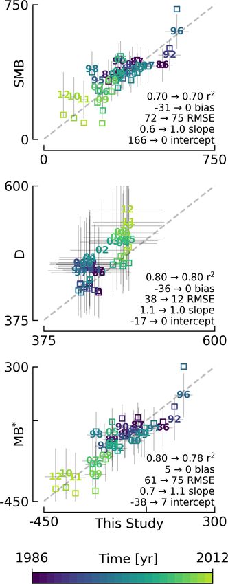
5006                                                   K. D. Mankoff et al.: Greenland mass balance 1840 through next week

   As the recent SMB decrease (successfully evaluated with         0.30/0.55 are applied to the bare ice albedo, representing ice
GRACE-based estimates in Fettweis et al., 2020) has been           with high-/low-impurity content (cryoconite, algae).
fully driven by the increase in runoff (Sasgen et al., 2020), we      To simulate as accurately as possible the contemporary
assume the same degree of accuracy between SMB simulated           climate and surface mass balance of the ice sheet, the fol-
by MAR (evaluated with the PROMICE SMB database in                 lowing boundary conditions have been applied. The glacier
Fettweis et al., 2020) and the runoff simulated by MAR.            ice mask and surface topography have been downsampled
   Weather-forecasted SMB. To provide a real-time state of         from the 90 m-resolution Greenland Ice Mapping Project
the Greenland ice sheet, MAR is forced automatically every         (GIMP) digital elevation model (DEM) (Howat et al., 2014).
day by the run of 00:00 UTC from the Global Forecast Sys-          At the lateral boundaries, model temperature, specific humid-
tem (GFS) model providing weather forecasting initialized          ity, pressure, and horizontal wind components at the 40 ver-
by the snowpack behaviors of the MAR run from the pre-             tical model levels are relaxed towards 6-hourly ECMWF re-
vious day. This continuous GFS-forced time series (without         analysis (ERA) data. For this we use ERA-40 between 1958
any reinitialization of MAR) provides SMB and runoff es-           and 1978 (Uppala et al., 2005), ERA-Interim between 1979
timates between the period covered by ERA5 and the next            and 1989 (Dee et al., 2011), and ERA-5 between 1990 and
7 d. At the end of each day, ERA5 is used to update the            2020 (Hersbach et al., 2020). The relaxation zone is 24 grid
GFS-forced MAR time series until about 5 d before the cur-         cells (∼ 130 km) wide to ensure a smooth transition to the
rent date and to provide a homogeneous ERA5-forced MAR             domain interior. This run has active upper-atmosphere relax-
times series from 1950 to a few days before the current date.      ation (van de Berg and Medley, 2016). Over glaciated grid
We use both the forecasted SMB and forecasted runoff (for          points, surface aerodynamic roughness is assumed constant
BMBVHD ) fields.                                                   for snow (1 mm) and ice (5 mm). In this run, RACMO2.3p2
                                                                   has 5.5 km horizontal resolution over Greenland and the ad-
                                                                   jacent oceans and land masses, but it was found previously
4.1.3   RACMO                                                      that this is insufficient to resolve the many narrow outlet
                                                                   glaciers. The 5.5 km product is therefore statistically down-
RACMO v2.3p2 has been developed at the Koninklijk Ned-             scaled onto a 1 km grid sampled from the GIMP DEM (Noël
erlands Meteorologisch Instituut (Royal Netherlands Mete-          et al., 2019), employing corrections for biases in elevation
orological Institute; KNMI). It incorporates the dynamical         and bare ice albedo using a MODIS albedo product at 1 km
core of the High-Resolution Limited Area Model (HIRLAM)            resolution (Noël et al., 2016).
and the physics parameterizations of the ECMWF Inte-
grated Forecast System cycle CY33r1. A polar version (p) of        4.1.4   Reconstruction
RACMO has been developed at the Institute for Marine and
Atmospheric research of Utrecht University (UU-IMAU) to            The Kjeldsen et al. (2015) 173-year (1840 through 2012)
assess the surface mass balance of glaciated surfaces. The         mass balance reconstruction is based on the Box (2013) 171-
current version RACMO2.3p2 has been described in detail            year (1840 through 2010) statistical reconstruction. Kjeldsen
in Noël et al. (2018), and here we repeat the main character-      et al. (2015) add a more sophisticated meltwater retention
istics.                                                            scheme (Pfeffer et al., 1991), weighting of in situ records in
   The ice sheet has an extensive dry interior snow zone, a        their contribution to the estimated value, and dispersal of an-
relatively narrow runoff zone along the low-lying margins,         nual accumulation to monthly and extend the reconstruction
and a percolation zone of varying width in between. To cap-        in time through 2012.
ture these processes on first order, the original single-layer        The Box (2013) 171-year (1840–2010) reconstruction is
snow model in RACMO has been replaced by a 40-layer                developed from linear regression parameters that describe
snow scheme that includes expressions for dry snow densifi-        the least squares regression between (a) spatially discontinu-
cation and a simple tipping bucket scheme to simulate melt-        ous in situ monthly air temperature records (Cappelen et al.,
water percolation, retention, refreezing, and runoff (Ettema       2011, 2006; Cappelen, 2001; Vinther et al., 2006) or firn/ice
et al., 2010). The snow layers were initialized in Septem-         cores (Box et al., 2013) and (b) spatially continuous outputs
ber 1957 using temperature and density from a previous run         from the regional climate model RACMO version 2.1 (Et-
with the offline IMAU Firn Densification Model (Ligtenberg         tema et al., 2010). A 43-year overlap period (1960 through
et al., 2018). To simulate drifting snow transport and subli-      2012) with the RACMO data is used to determine regres-
mation, Lenaerts et al. (2012) implemented a drifting snow         sion parameters (slope, intercept) on a 5 km grid cell basis.
scheme. Snow albedo depends on snow grain size, cloud              Temperature data define melting degree days, which have a
optical thickness, solar zenith angle, and impurity content        different coefficient for bare ice than snow cover, determined
(van Angelen et al., 2012). Bare ice albedo is assumed con-        from hydrological-year cumulative SMB. A fundamental as-
stant and estimated as the 5th percentile value of albedo time     sumption is that the calibration factors, regression slope, and
series (2000–2015) from the 500 m-resolution MODIS 16 d            offset for the calibration period 1960 through 2012 are sta-
albedo product (MCD43A3). Minimum/maximum values of                tionary over time, for which there is some evidence in Fet-

Earth Syst. Sci. Data, 13, 5001–5025, 2021                                         https://doi.org/10.5194/essd-13-5001-2021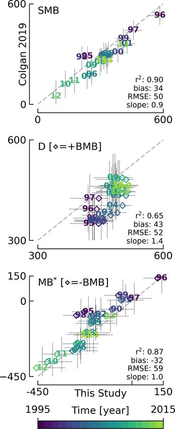
K. D. Mankoff et al.: Greenland mass balance 1840 through next week                                                               5007

                                                                        The discharge in Mankoff et al. (2020b) is computed at flux
                                                                        gates ∼ 5 km upstream from glacier termini (Mankoff, 2020)
                                                                        using a wide range of velocity products and ice thickness
                                                                        from BedMachine v4. Discharge across flux gates is derived
                                                                        with a 200 m spatial resolution grid but then summed and
                                                                        provided at glacier resolution. Temporal coverage begins in
                                                                        1986 with a few velocity estimates and is updated each time a
                                                                        new velocity product is released, which is every ∼ 12 d with
                                                                        a ∼ 30 d lag (Solgaard et al., 2021; data: Solgaard and Kusk,
                                                                        2021).
                                                                           Some changes have been implemented since the last pub-
                                                                        lication describing the discharge product (i.e., Mankoff et al.,
                                                                        2020b). These are minor and include updating the Khan
                                                                        et al. (2016) (data: Khan, 2017) surface elevation change
                                                                        product from 2015 through 2019, updating various MEa-
                                                                        SUREs velocity products to their latest version, updating
                                                                        the PROMICE Sentinel ice velocity product from Edition 1
                                                                        (https://doi.org/10.22008/promice/data/sentinel1icevelocity/
                                                                        greenlandicesheet/v1.0.0) to Edition 2 (Solgaard et al., 2021;
                                                                        Solgaard and Kusk, 2021), and updating from BedMachine
                                                                        v3 (supplemented in the SE with Millan et al., 2018) to use
                                                                        only BedMachine v4 (Morlighem et al., 2021).
                                                                           The reconstructed discharge data (Kjeldsen et al., 2015)
                                                                        are estimated via a linear fit between unsmoothed annual
                                                                        discharge spanning 2000 to 2012 (Enderlin et al., 2014) and
                                                                        runoff data from Kjeldsen et al. (2015) using a 6-year trail-
                                                                        ing average. The method for scaling discharge from runoff
                                                                        was introduced by Rignot et al. (2008), who scaled the SMB
                                                                        anomaly with discharge. Sensitivity analyses conducted by
                                                                        Box and Colgan (2013) showed runoff to be the more ef-
                                                                        fective discharge predictor and include a discussion of the
                                                                        physical basis. Although the fitting period of the present data
                                                                        set includes an anomalous period of discharge (2000 through
                                                                        2005; e.g., Boers and Rypdal, 2021), the discharge data used
Figure 3. Comparison between This Study and the reconstruction          by Rignot et al. (2008) and Box and Colgan (2013) also in-
(Kjeldsen et al., 2015). All axis units are Gt yr−1 . Plotted numbers   clude years 1958 and 1964 that lie near the regression line
represent the last two digits of the years for the unadjusted data      (see Box and Colgan, 2013, Fig. 4, and the related Sect. 4,
sets. The matching colored squares show the adjusted data. MB∗          Physical basis). Further, while 2000 through 2005 cover a
shown here does not include BMB for either the reconstructed or         changing period in Greenlandic discharge (Mankoff et al.,
This Study data. Arrows show statistical properties before and after    2020b; King et al., 2020), there were likely other anomalous
the adjustment. No adjustment is made to MB∗ , but it is computed       periods in the past, when glaciers in Greenland experienced
from Eq. (4) both before (numbered) and after (squares) the surface     considerable increases in discharge, as inferred by geologi-
and discharge adjustments.                                              cal and geodetic investigations (Andresen et al., 2012; Bjørk
                                                                        et al., 2012; Khan et al., 2015, 2020).
                                                                           The reconstructed discharge is adjusted as described in the
tweis et al. (2017). Box et al. (2013) describe the methods in          Methods Sect. 5.4.
more detail.
   The reconstructed surface mass balance is adjusted as de-
                                                                        4.3   Basal mass balance
scribed in the Methods Sect. 5.4 (Fig. 3).
                                                                        The BMB (Karlsson et al., 2021) comes from mass lost at
                                                                        the bed from BMBGF , BMBfriction from the basal shear ve-
4.2   Discharge
                                                                        locity, and BMBVHD from surface runoff routed to the bed
The recent discharge data are from Mankoff et al. (2020b)               (i.e., the volume of the subglacial conduits formed from sur-
(data: Mankoff and Solgaard, 2020). This product covers                 face runoff; Mankoff and Tulaczyk, 2017).
all fast-flowing (> 100 m yr−1 ) marine-terminating glaciers.

https://doi.org/10.5194/essd-13-5001-2021                                              Earth Syst. Sci. Data, 13, 5001–5025, 2021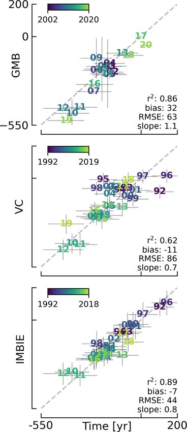
5008                                                    K. D. Mankoff et al.: Greenland mass balance 1840 through next week

   These fields (data: Karlsson, 2021) are provided as steady-      4.5    Products used for validation
state annual estimates. We use the BMBGF and BMBfriction
                                                                    We validate This Study against five other data products (see
products and apply 1/365th to each day, each year. Because
                                                                    Table 2 and Sect. 6). These products are the most recent
BMBVHD is proportional to runoff, an annual estimate is not
                                                                    IO product (Mouginot et al., 2019), the previous PROMICE
appropriate for this work with daily resolution. We therefore
                                                                    mass balance product (Colgan et al., 2019; data: Colgan,
re-calculate the BMBVHD -induced basal melt as described in
                                                                    2021), the two mostly independent methods of estimating ice
the Methods Sect. 5.3.
                                                                    sheet mass change, GMB (Barletta et al., 2013; data: Barletta
                                                                    et al., 2020) and VC (Simonsen et al., 2021a; data: Simonsen
4.3.1    Geothermal flux
                                                                    et al., 2021b), and the IMBIE2 data (IMBIE Team, 2019). In
Due to a lack of direct observations, the geothermal flux is        addition to this, we evaluate the reconstructed Kjeldsen et al.
poorly constrained under most of the Greenland ice sheet.           (2015) (data: Box et al., 2021) and This Study data during
Different approaches have been employed to infer the value          the overlapping period 1986 through 2012.
of the BMBGF , often with diverging results (see, e.g., Ro-
gozhina et al., 2012; Rezvanbehbahani et al., 2019). Lacking        5     Methods
substantial validation that favors one BMBGF map over the
others, Karlsson et al. (2021) instead use the average of three     The total mass balance for all of Greenland and all the dif-
widely used BMBGF estimates: Fox Maule et al. (2009),               ferent ROIs involves summing each field (SMB, D, BMB)
Shapiro and Ritzwoller (2004), and Martos et al. (2018). The        by each ROI and then subtracting the D and BMB from the
BMBGF melt rate is calculated as                                    SMB fields, or
ḃm = EGF ρi−1 L−1 ,                                         (1)    MB = SMB − D − BMB.                                        (3)
where EGF is available energy at the bed, here the geothermal          Products that do not include the BMB term (i.e., Mouginot
flux in unit W m−2 , ρi is the density of ice (917 kg m−3 ), and    et al., 2019, Colgan et al., 2019, and Kjeldsen et al., 2015)
L is the latent heat of fusion (335 kJ kg−1 ; Cuffey and Pater-     have total mass balance defined as
son, 2010). BMBGF melting is only calculated where the bed
                                                                    MB∗ = SMB − D,                                             (4)
is not frozen. We use the MacGregor et al. (2016) estimate of
temperate bed extent and scale Eq. (1) by 0, 0.5, or 1 where        and when comparing This Study to those products, we com-
the bed is frozen (∼ 25 % of the ice sheet area), uncertain         pare like terms, never comparing our MB to a different prod-
(∼ 33 %), or thawed (∼ 42 %), respectively.                         uct MB∗ , except in Fig. 4, where all products are shown to-
                                                                    gether.
4.3.2    Friction                                                     Prior to calculating the mass balance, we perform the fol-
                                                                    lowing steps.
This heat term stems from the friction produced as ice slides
over the bedrock. The term has only been measured in a              5.1    Surface mass balance
handful of places (e.g., Ryser et al., 2014; Maier et al., 2019),
and it is unclear how representative those measurements are         In This Study we generate an output based on each of the
at ice sheet scales. Karlsson et al. (2021) therefore estimate      three RCMs (HIRHAM/HARMONIE, MAR, and RACMO);
the frictional heating using the full Stokes Elmer/Ice model        however, in addition to these we generate a final and fourth
that resolves all stresses while relating basal sliding and shear   SMB field defined as a combination of (1) the adjusted
stress using a linear friction law (Gillet-Chaulet et al., 2012;    reconstructed SMB from 1840 through 1985 (Sect. 5.4)
Maier et al., 2021). The model is tuned to match a multi-           and (2) the average of HIRHAM/HARMONIE, MAR, and
decadal surface velocity map (Joughin et al., 2018) covering        RACMO from 1986 through a few months ago, the average
1995–2015, and it returns an estimated basal friction heat that     of HIRHAM/HARMONIE and MAR from a few months ago
is used to calculate the basal melt due to friction, similarly to   through yesterday, and MAR from yesterday through next
Eq. (1):                                                            week. See Appendix A for differences between This Study
                                                                    MB and MB derived using each of the RCM SMBs. There
ḃm = Ef ρi−1 L−1 ,                                          (2)
                                                                    is no obvious change or step function at the 1985 to 1986
where Ef is energy due to friction. We also apply the 0, 0.5,       reconstructed-to-recent change nor as the RACMO and then
and 1 scale as used for the BMBGF term (MacGregor et al.,           HIRHAM/HARMONIE RCMs become unavailable a few
2016) in order to mask out areas that are likely frozen.            months ago and yesterday, respectively.

4.4     Other                                                       5.2    Projected discharge
ROI regions come from Mouginot and Rignot (2019) and                We project the discharge from the last observed point from
ROI sectors come from Zwally et al. (2012).                         Mankoff et al. (2020b) (generally between 2 weeks and

Earth Syst. Sci. Data, 13, 5001–5025, 2021                                          https://doi.org/10.5194/essd-13-5001-2021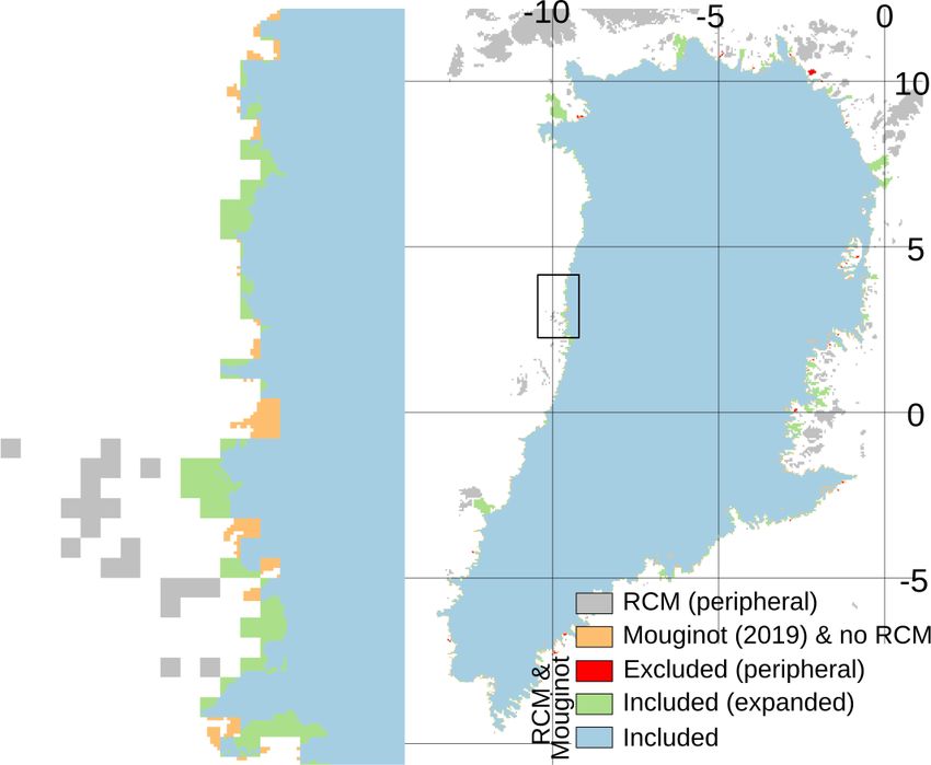
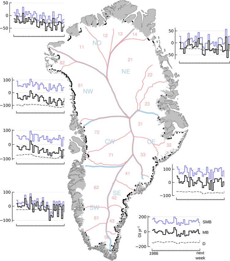
K. D. Mankoff et al.: Greenland mass balance 1840 through next week                                                                     5009

Table 2. Summary of correlation, bias, and RMSE between different products during their overlap periods with This Study. Basal mass
balance not included in This Study when comparing against Mouginot and Rignot (2019), Colgan et al. (2019), or Kjeldsen et al. (2015).
Peripheral ice masses never included in This Study.

   Other product               r2     Bias    RMSE      Figure    Overlap        Notes
   Mouginot et al. (2019)     0.94     11       38         5      1986–2018      No basal mass balance
   Colgan et al. (2019)       0.87    −32       59         6      1995–2015      No basal mass balance
   GMB                        0.86     32       63         7      2002–2020      Includes peripheral masses
   VC                         0.62    −11       86         7      1992–2019      Multi-year smooth
   IMBIE2                     0.89     −7       44         7      1992–2018      No BMB when using IO; BMB when using GMB or VC
   Kjeldsen et al. (2015)     0.80      5       61         3      1986–2012      No basal mass balance; includes peripheral masses

Figure 4. Comparison between This Study and other mass balance time series. Note that various products do or do not include basal mass
balance or peripheral ice masses (see Table 2). This Study annual-resolution data prior to 1986 are the Kjeldsen et al. (2015) data adjusted as
described in Sect. 5.4. Sea level rise calculated as −Gt/361.8. Inset highlights changes since 2010. Data product version 74 from 25 October
2021 used to generate this graphic.

1 month old) to 7 d into the future at each glacier. We define            et al., 2018), but surface mass balance changes sign and has
the long-term trend as the linear least squares fit to the last           both larger and higher frequency variability. From this, the
3 years of data. The residual is the data minus the long-term             statistical forecast for discharge described above does not im-
trend. We define the seasonal signal as the daily average from            pact results as much as the physically based model forecast
each year of the last 3 years of the residual during the tem-             for surface mass balance.
poral window of interest that spans from the most recently
available observation through next week. We shift the sea-
sonal signal so that it is 0 on the first projected day. We then          5.3   Basal mass balance
assign the value of the last observation, plus the long-term              Because Karlsson et al. (2021) provide a steady-state annual-
trend, plus the seasonal signal to the recent past-projected              average estimate of the BMB fields, we divide the BMBGF
and future-forecasted D.                                                  and BMBfriction fields by 365 to estimate daily average. This
   Discharge does not change sign and changes magnitude by                is a reasonable treatment of the BMBGF field, which does
approximately 6 % annually over the entire ice sheet (King                not have an annual cycle. The BMBfriction field does have a

https://doi.org/10.5194/essd-13-5001-2021                                                  Earth Syst. Sci. Data, 13, 5001–5025, 2021
5010                                                  K. D. Mankoff et al.: Greenland mass balance 1840 through next week

small annual cycle that matches the annual velocity cycle.        two has an r 2 value of 0.75, a slope of 0.03, and an intercept
However, when averaged over all of Greenland, this is only a      of −3 Gt yr−1 (Appendix D). From this, we scale the Kjeld-
∼ 6 % variation (King et al., 2018), and Karlsson et al. (2021)   sen et al. (2015) reconstructed runoff by 3 % (from the 0.03
found that basal melt rates are 5 % higher during the summer.     slope, unrelated to the theoretical 1000 m drop described ear-
Thus, the intra-annual changes are less than the uncertainty.     lier) to estimate reconstructed BMBVHD .
The BMBVHD field varies significantly throughout the year,
because it is proportional to surface runoff. We therefore gen-   5.4   Reconstructed adjustment
erate our own BMBVHD for This Study.
   To estimate recent BMBVHD , we use daily MAR runoff            We use the reconstructed and recent SMB and D overlap
(see Mankoff et al., 2020a) and BedMachine v4 (Morlighem          from 1986 through 2012 to adjust the reconstructed data.
et al., 2017, 2021) to derive subglacial routing pathways,        This Study vs. reconstructed SMB has a slope of 0.6 and
similarly to Mankoff and Tulaczyk (2017). We assume that          an intercept of 166 Gt yr−1 (Fig. 3 SMB), and This Study
all runoff travels to the bed within the grid cell where it is    vs. reconstructed D has a slope of 1.1 and an intercept of
generated, the bed is pressurized by the load of the over-        −17 Gt yr−1 (Fig. 3 D). The unadjusted reconstructed data
head ice, and the runoff discharges on the day it is generated.   slightly underestimate years with high SMB and overesti-
We calculate subglacial routing from the gradient of the sub-     mate years with low SMB (see 1986, 2010, 2011, and 2012
glacial pressure head surface, h, defined as                      in Fig. 3 SMB). The unadjusted reconstructed data slightly
                                                                  overestimate years with low D and overestimate years with
             ρi
h = zb + k      (zs − zb ),                                (5)    high D.
             ρw                                                      We adjust the reconstructed data until the reconstructed vs.
with zb the basal topography, k the flotation fraction (1),       recent slope is 1 and the intercept is 0 Gt yr−1 for each of the
ρi the density of ice (917 kg m−3 ), ρw the density of water      surface mass balance and discharge comparisons (Fig. 3). We
(1000 kg m−3 ), and zs the ice surface. Equation (5) comes        then derive the BMBVHD term for reconstructed basal mass
from Shreve (1972), where the hydropotential has units of         balance (Sect. 5.3 and Appendix D), bring in the other BMB
Pascals (Pa), but here it is divided by gravitational accelera-   terms (Sect. 5.3), and use Eq. (3) to compute the adjusted
tion g times the density of water ρw to convert the units from    reconstructed mass balance.
Pascals to meters (Pa to m).                                         For reconstructed SMB and D, the mean of the recent un-
   We compute h and from h streams and outlets and both           certainty is added to the reconstructed uncertainty during
the pressure and elevation difference between the source and      the adjustment. Reconstructed MB uncertainty is then re-
outlet. The energy available for basal melting is the eleva-      calculated as the square root of the sum of the squares of
tion difference (gravitational potential energy) and two-thirds   the reconstructed SMB and D uncertainty.
of the pressure difference, with the remaining one-third con-        For surface mass balance, the adjustment is effectively a
sumed to warm the water to match the changing phase tran-         rotation around the mean values, with years with low SMB
sition temperature (Liestøl, 1956; Mankoff and Tulaczyk,          decreasing and years with high SMB increasing after the ad-
2017). We assume all energy, EVHD (in Joules), is used to         justment. For discharge, years with low D are slightly re-
melt ice with                                                     duced, and years with high D have a higher reduction to bet-
                                                                  ter match the overlapping estimates.
bm = EVHD ρi−1 L−1 .                                       (6)       The adjustment described above treats all biases in the re-
                                                                  constructed data. The primary assumption of our adjustment
   Because results are presented per ROI, and to reduce the       is that the bias contributions do not change in proportion to
computational load of this daily estimate, we only calcu-         each other over time. We attribute the disagreement and need
late the integrated energy released between the RCM runoff        for the adjustment to the demonstrated too-high biases in ac-
source cell and the outlet cell and then assign that to the ROI   cumulation and ablation estimates in the 1840–2012 recon-
containing the runoff source cell.                                structed SMB field (Fettweis et al., 2020), an offset resulting
   To estimate reconstructed basal mass balance, we treat         from differences in ice masks (Kjeldsen et al., 2015), the in-
BMBGF and BMBfriction as steady state as described at the         clusion of peripheral glaciers (Kjeldsen et al., 2015), other
start of this section. For BMBVHD we use the fact that VHD        accumulation rate inaccuracies (Lewis et al., 2017, 2019),
comes from runoff by definition, and from this, reconstructed     and other unknowns.
BMBVHD is calculated using scaled runoff as a proxy. VHD
theory suggests that a unit volume of runoff that experiences     5.5   Domains, boundaries, and regions of interest
a 1000 m elevation drop will release enough heat to melt an
additional 3 % (Liestøl, 1956). To estimate the scale factor,     Few of the ice masks used here are spatially aligned. The
we use the 1986 through 2012 overlap between the Kjeldsen         Zwally et al. (2012) sectors and the Mouginot and Rignot
et al. (2015) runoff and This Study recent BMBVHD from            (2019) regions are often smaller than the RCM ice domains.
MAR runoff described above. The correlation between the           For example, the RACMO ice domain is 1 718 959 km2 , of

Earth Syst. Sci. Data, 13, 5001–5025, 2021                                        https://doi.org/10.5194/essd-13-5001-2021
K. D. Mankoff et al.: Greenland mass balance 1840 through next week 5011
which 1 696 419 km2 (99 %) are covered by the Mouginot (SMB, D, and MB∗ ) comparison and the GMB, VC, and IM-
and Rignot (2019) regions and 22 540 km2 (1 %) are not, or BIE2 only MB-level comparison. The MB or MB∗ compar-
1 678 864 km2 (98 %) are covered by Zwally et al. (2012) and ison for each product is summarized in Table 2. PAll have
40 095 km2 (2 %) are not. different masks. Bias (Gt yr−1 ) is defined as n1 ni=1 (xi −
Cropping the RCM domain edges would remove the edge yi ).qRoot mean square error (RMSE) (Gt yr−1 ) is defined
cells where the largest SMB losses occur. This effect is mi- as n1 ni=1 (xi − yi )2 . Sums are computed using ice-sheet-
P
nor when SMB is high (years with low runoff, assuming wide annual values, where x is This Study, y is the other
SMB magnitude is dominated by the runoff term). This ef- product, and a positive bias means that This Study has a
fect is large when SMB is low (years with high runoff). larger value.
As an example of the 2010 decade, RACMO SMB has a
mean of 251 Gt yr−1 for the decade, with a low of 45 Gt in
6.1 Mouginot (2019)
2019 and a high of 420 Gt in 2018. For these same extreme
years RACMO cropped to Mouginot and Rignot (2019) has The Mouginot et al. (2019) product spans the 1972 through
a low of 76 Gt (68 % high) and a high of 429 Gt (2 % high). 2018 period. We only use 1986 and onward because This
RACMO cropped to Zwally et al. (2012) has a low of 84 Gt Study has annual resolution prior to 1986 and Mouginot et al.
(85 % high) and a high of 429 Gt (2 % high). (2019) data are provided on a non-calendar-year period. The
We therefore grow the ROIs to cover the RCM domains. SMB comes from RACMO v2.3p2 downscaled at 1 km and
ROIs are grown by expanding them outward, assigning the agrees very well with SMB from This Study (r 2 0.94, bias 11,
new cells the value (ROI classification, that is, sector num- RMSE 38, slope 1.1). The minor SMB differences are likely
ber or region name; see Fig. 1) of the nearest non-null cell, due to mask differences or our use of a three-RCM average
and then clipping to the RCM ice domain. This is done for SMB estimate.
each ROI and RCM. Appendix E provides a graphical dis- Mouginot et al. (2019) discharge and our D from Mankoff
play of the HIRHAM RCM domain, the Mouginot and Rig- et al. (2020b) have a −33 Gt yr−1 bias. This difference can
not (2019) domain, and our expanded Mouginot and Rignot mainly be attributed to different discharge estimates in the
(2019) domain. southeastern and central eastern sectors (Appendix: Moug-
BMBVHD comes from the MAR ice domain runoff but is inot regions). When we include BMB in This Study (dia-
generated on the BedMachine ice thickness grid, which is monds in middle panel of Fig. 5 shifting values to the right),
smaller than the ice domain in some places. Therefore, the it adds ∼ 25 Gt yr−1 to This Study.
largest runoff volumes per unit area (from the low-elevation Because MB∗ is a linear combination of SMB and D terms
edge of the ice sheet) are discarded in these locations. (Eq. 4), the MB∗ differences between this product and Moug-
inot et al. (2019) are dominated by the D term, although it is
not apparent because interannual variability is dominated by
6 Product evaluation and assessment SMB.
We compare to six related data sets (see Table 2 and
6.2 Colgan (2019)
Sect. 4.5): the most similar and recent IO product (Mouginot
et al., 2019), the previous PROMICE assessment (Colgan The Colgan et al. (2019) product spans 1995 through 2015.
et al., 2019), the two mostly independent methods (GMB, The SMB term is broadly similar to the RCM-averaged SMB
Barletta et al., 2013, and VC, Simonsen et al., 2021a), term in This Study, although Colgan et al. (2019) use only an
IMBIE2 (IMBIE Team, 2019), and the unadjusted recon- older version of MAR (Fig. 6 top panel). The Colgan et al.
structed/recent overlap (Kjeldsen et al., 2015). (2019) SMB is spatially interpolated over the PROMICE ice
Our initial comparison (Fig. 4) shows all seven products sheet ice mask (Citterio and Ahlstrøm, 2013), which contains
overlaid in a time series accumulating at the product resolu- more detail on the ice sheet periphery and therefore a larger
tion (daily to annual) from the beginning of the first overlap ablation area than the native coarser MAR ice mask. This
(1972, Mouginot et al., 2019) until 7 d from now (now de- Study does not interpolate the SMB field and instead works
fined as 25 October 2021 based on the date this document on the SMB ice domain.
is compiled). Each data set is manually aligned vertically The largest difference between This Study and Colgan
so that the last timestamps appear to overlap, allowing dis- et al. (2019) is that the latter estimate grounding line ice dis-
agreements to grow back in time. We also assume errors are charge based on corrections to ice volume flow rate measured
smallest at present and allow errors to grow back in time. across the ∼ 1700 m elevation contour. This is far inland rel-
The errors for this product are described in the Uncertainty ative to the grounding line flux gates used in This Study
section. (from Mankoff, 2020). This introduces uncertainty into the
In the sections below, we compare This Study to each Colgan et al. (2019) D term from SMB corrections between
of the validation data in more detail. The Mouginot et al. the 1700 m elevation contour and the terminus (see the large
(2019) and Colgan et al. (2019) products allow term-level disagreement in Fig. 6 middle panel). This disagreement in-
https://doi.org/10.5194/essd-13-5001-2021 Earth Syst. Sci. Data, 13, 5001–5025, 20215012 K. D. Mankoff et al.: Greenland mass balance 1840 through next week
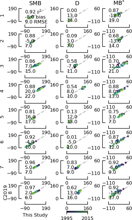
Figure 5. Comparison of This Study vs. Mouginot et al. (2019). All Figure 6. Comparison of This Study vs. Colgan et al. (2019). All
axis units are Gt yr−1 . Plotted numbers represent the last two digits axis units are Gt yr−1 . Plotted numbers represent the last two digits
of the year. Matching colored diamonds show the data when BMB of the year. Matching colored diamonds show the data when BMB
is added to This Study. Printed numbers (r 2 , bias, RMSE, slope) is added to This Study. Printed numbers (r 2 , bias, RMSE, slope)
compare values without BMB. compare values without BMB.
creases when BMB is included in the results of This Study ing the earliest part of the record (i.e., 1995–2000), decreas-
(shown by the annual values shifting to the right). ing towards the present day, which may suggest that Colgan
The D disagreement is represented differently across sec- et al. (2019) particularly overestimated the response in ice
tors (Appendix: Colgan 2019), where sectors 1, 2, 5, and 6 discharge to 1990s climate variability.
all have correlation coefficients less than ∼ 0.1, while the re- Similarly to the comparison with Mouginot et al. (2019),
maining sectors 3, 4, 7, and 8 all have correlation coefficients the disagreement between This Study and Colgan et al.
greater than 0.5. (2019) is dominated by D disagreement, although it is again
This Study assesses greater D bias (43 Gt yr−1 ) than Col- not apparent because interannual variability is dominated by
gan et al. (2019). While Colgan et al. (2019) did not assess SMB.
BMB, the majority of this discrepancy likely results from
Colgan et al. (2019) aliasing the aforementioned downstream 6.3 GMB
correction terms. For example, while This Study shows very
little interannual variability in ice discharge in the predomi- Unlike This Study, the GMB method includes mass losses
nantly land-terminating SW region, Colgan et al. (2019) infer and gains on peripheral ice masses which should introduce
large interannual variability in ice discharge based on large a bias of ∼ 10 % to 15 % (Colgan et al., 2015; Bolch et al.,
interannual variability in SMB and changes in ablation area 2013). The inclusion of peripheral ice in the GMB product
ice volume in their Sector 6. The discrepancy between This is because the spatial resolution is so low that it cannot dis-
Study and the Colgan et al. (2019) D[+BMB] is largest dur- tinguish between them and the main ice sheet. There is also
Earth Syst. Sci. Data, 13, 5001–5025, 2021 https://doi.org/10.5194/essd-13-5001-2021K. D. Mankoff et al.: Greenland mass balance 1840 through next week 5013
signal leakage from other glaciated areas, e.g., the Canadian
Arctic. This can have an effect on the estimated signal, es-
pecially in sectors 1 and 8 or regions NW and NO. There
is also leakage between basins, which becomes a larger is-
sue for smaller basins or where major outlet glaciers are near
basin boundaries. GMB may also have an amplified seasonal
signal due to changing snow loading in the surrounding land
areas that may be mapped as ice sheet mass change variabil-
ity. This would enhance the seasonal amplitude but not have
an impact on the interannual mass change rates. Addition-
ally, different glacial isostatic adjustment (GIA) corrections
applied to the gravimetric signal may also lead to differences
in GMB estimates on an ice sheet scale but also on a sector
scale (e.g., Sutterley et al., 2014; Khan et al., 2016).
GMB and the IO method (This Study) both report changes
in ice sheet mass, but they are measuring two fundamen-
tally different things. The IO method tracks volume flow rate
across the ice sheet boundaries. Typically this is meltwater
across the ice sheet surface and solid ice across flux gates
near the calving edge of the ice sheet, and in This Study also
meltwater across the ice sheet basal boundary. That volume
is then converted to mass. We consider that mass is “lost”
as soon as it crosses the boundary (i.e., the ice melts or ice
crosses the flux gate). The GMB method tracks the regional
mass changes. Melting ice has no impact on this until the
meltwater enters the ocean and a similar mass leaves the
far-field GMB footprint. From these differences, the GMB
method may be a better estimate of sea level rise, while the
IO method may be a better representation of the state of the Figure 7. This Study total mass balance (MB) vs. the gravimetric
Greenland ice sheet. method (GMB), volume change method (VC), and IMBIE2 esti-
mates of MB. All three include BMB. All axis units are Gt yr−1 .
6.4 VC Plotted numbers represent the last two digits of the year. GRACE
and IMBIE2 include peripheral ice masses.
When deriving surface elevation change from satellite al-
timetry, data from multiple years are needed to give a sta-
ble ice-sheet-wide prediction. Hence, the altimetric mass bal-
ance estimates are often reported as averages of single satel- et al. (2021a) used a machine learning approach to derive
lite missions. a temporal calibration field for converting the radar eleva-
Although This Study has a small (−11 Gt yr−1 ) bias in tion change estimates into mass change. This approach re-
comparison to Simonsen et al. (2021a) VC, there is a rela- lied on precise mass balance estimates from ICESat to train
tively high RMSE of 86 Gt yr−1 and a mid-range correlation the model and thereby was able to remove the effects of the
(r 2 = 0.62). This suggests that while both This Study and changing scattering horizon in the radar data. This VC mass
VC agree on the total mass loss of the ice sheet, they dis- balance is given for monthly time steps (Simonsen et al.,
agree on the precise temporal distribution of this mass loss. 2021a); however, the running mean applied to derive radar
It is possible that the outlying 1992 and 2019 years are influ- elevation change will dampen the interannual variability of
enced by the edge of the time series record if not fully sam- the mass balance estimate from VC. This is especially true
pled, but other outliers exist – the 1992 extreme low melt year prior to 2010, after which the novel radar altimeter onboard
and the 2019 extreme melt year as well as the 1995 through CryoSat-2 allowed for a shortening of the data windowing
1998 period stand out as years with poor agreement. from 5 to 3 years. This smoothing of the interannual variabil-
We suggest that this is due to climate influences on the ity is also seen in the intercomparison between This Study
effective radar horizon across the ice sheet during these and the VC MB, where in addition to the two end-members
years. Weather-driven change in the effective scatter hori- of the time series (1992 and 2019) the years 1995, 1996, and
zon, mapped by the Ku band in the upper snow layer of 1998 seem to be outliers (Fig. 7). These years are notable for
ice sheets, hampers the conversion of radar-derived elevation high MB, which seems to be captured less precisely by the
change into mass change (Nilsson et al., 2015). Simonsen older radar altimeters due to the longer temporal averaging.
https://doi.org/10.5194/essd-13-5001-2021 Earth Syst. Sci. Data, 13, 5001–5025, 20215014 K. D. Mankoff et al.: Greenland mass balance 1840 through next week
6.5 IMBIE the last Mankoff et al. (2020b) D data (up to 30 d old, with
an error of ∼ 9 % or ∼ 45 Gt yr−1 ) and the forecasted now-
The most widely cited estimate of Greenland mass balance plus-7 d D (see Sect. 7.1). Table 3 provides a summary of the
today is the Ice-Sheet Mass Balance Inter-Comparison Exer- uncertainty for each input.
cise 2 (IMBIE2, IMBIE Team, 2019). IMBIE2 seeks to pro- The final This Study MB uncertainty value shown in Ta-
vide a consensus estimate of monthly Greenland mass bal- ble 3 comes from the mean of the annual sum of the MB error
ance between 1992 and 2018 that is derived from altimetry, term.
gravimetry, and input–output ensemble members. There are
two critical methodological differences between This Study
and IMBIE2. Firstly, the gravimetry members of IMBIE2 as- 7.1 Discharge
sess the mass balance of all Greenlandic land ice, including The D uncertainty is discussed in detail in Mankoff et al.
peripheral ice masses, while This Study only assesses the (2020b), but the main uncertainties come from unknown
mass balance of the ice sheet proper. Secondly, the input– ice thickness, the assumption of no vertical shear at fast-
output members of IMBIE2 do not assess BMB, while This flowing marine-terminating outlet glaciers, and ice density
Study does. of 917 kg m−3 . Regional ice density can be significantly re-
The IMBIE2 composite record of ice sheet mass balance duced by crevasses. For example, Mankoff et al. (2020c)
equally weights three methods of assessing ice sheet mass identified a snow-covered crevasse field with 20 % crevasse
balance: input–output, altimetry, and gravimetry. Prior to ca. density, meaning at that location regional firn density should
2003, however, IMBIE2 is derived solely from IO studies be reduced by 20 %.
that explicitly exclude BMB (MB is actually MB∗ ). After ca. Temporally, D at daily resolution comes from ∼ 12 d ob-
2003, by comparison, IMBIE2 includes both satellite altime- servations upsampled to daily, and those ∼ 12 d resolution
try and gravimetry records implicitly sampling BMB. The observations come from longer time period observations
representation of BMB in the composite IMBIE2 mass bal- (Solgaard et al., 2021). Because the velocity method uses fea-
ance record therefore shifts before and after ca. 2003. ture tracking, it is correct on average but misses variability
In comparison to mass balance assessed by IMBIE2, This within each sample period (e.g., Greene et al., 2020).
Study has a small bias of ∼ -7 Gt yr−1 over the 26-calendar- Spatially, discharge is estimated ∼ 5 km upstream from
year comparison period. This apparent agreement may be at- the grounding lines for ice velocities as low as 100 m yr−1 .
tributed to the compensating effects of IMBIE2 effectively That ice accelerates toward the margin, but even ice flowing
sampling peripheral ice masses and ignoring BMB, while steadily at 1 km yr−1 would take 5 years before that mass is
This Study does the opposite and ignores peripheral ice lost. However, at any given point in time, ice that had pre-
masses but samples BMB, equal to ∼ 25 Gt yr−1 . Over the viously crossed the flux gate is calving or melting into the
entire 26-year comparison period, the RMSE with IMBIE2 is fjord. The discrepancy here between the flux gate estimated
44 Gt yr−1 and the correlation is 0.89. This relatively high mass loss and the actual mass lost at the downstream termi-
correlation highlights good agreement in interannual vari- nus is only significant for glaciers that have had large veloc-
ability between studies, and the RMSE suggests that formal ity changes at some point in the recent past, large changes
stated uncertainties of each study (ca. ±30 to ±63 Gt yr−1 in ice thickness, or large changes in the location (retreat or
for IMBIE2 and a mean of 86 Gt yr−1 for This Study) are in- advance) of the terminus. We do not consider SMB changes
deed good estimates of the true uncertainty, as assessed by downstream of the flux gate, because the gates are temporally
inter-study discrepancies. near the terminus for most of the ice that is fast-flowing, and
the largest SMB uncertainty is at the ice sheet margin, where
7 Uncertainty there are both mask issues and high topographic variability.
The forecasted D uncertainty is the average historical un-
We treat the three inputs to the total mass balance (sur- certainty plus a 1 % increase per day for the past projected
face mass balance, discharge, and basal mass balance, or and forecasted period.
SMB, D, and BMB) as independent when calculating the
total error. This is a simplification – the RCM SMB and 7.2 ROIs
the BMBVHD from RCM runoff are related and D ice thick-
ness and BMBVHD pressure gradients are related, and other We work on the three different domains of the three RCMs
terms may have dependencies. However, the two dominant and expand the ROIs to match the RCMs (see Appendix E).
IO terms, SMB inputs and D outputs, are independent on an- However, some alignment issues cannot be solved. For exam-
nual timescales, and for simplification we treat all terms as ple, we use BedMachine ice thickness to estimate BMBVHD .
independent. We use Eq. (3) and standard error propagation Often, the largest BMBVHD occurs near the ice margin un-
for SMB, D, and BMB terms (i.e., the square root of the sum der ice with the steepest surface slopes. This is also where
of the squares of the SMB plus D plus BMB error terms). the largest runoff often occurs, because the ice margin, at
For D, extra work is done to calculate uncertainty between the lowest elevations, is exposed to the warmest air. If these
Earth Syst. Sci. Data, 13, 5001–5025, 2021 https://doi.org/10.5194/essd-13-5001-2021You can also read